Special Issue: Human-environment interactions and Ecosystems

Variation of gross primary productivity dominated by leaf area index in significantly greening area

  • CHEN Xin , 1 ,
  • CAI Anning , 2, * ,
  • GUO Renjie 1 ,
  • LIANG Chuanzhuang 3 ,
  • LI Yingying 1
Expand
  • 1. School of Geographical Sciences, Nanjing University of Information Science and Technology, Nanjing 210044, China
  • 2. School of Tourism and Social Management, Nanjing Xiaozhuang University, Nanjing 211171, China
  • 3. School of Geographical Sciences, Nanjing Normal University, Nanjing 210024, China
* Cai Anning (1973-), PhD and Professor, specialized in urban and regional development. E-mail:

Chen Xin (1996-), PhD, specialized in ecological climatology. E-mail:

Received date: 2022-10-12

  Accepted date: 2023-04-11

  Online published: 2023-08-29

Supported by

National Natural Science Foundation of China(52078237)

Abstract

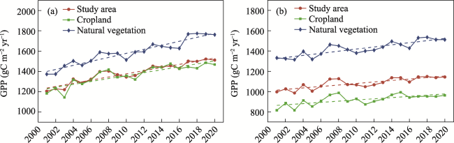
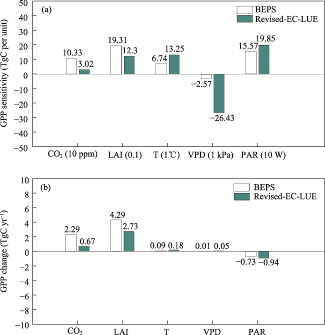
The leaf area index (LAI) shows a significant increasing trend from global to regional scales, which is known as greening. Greening will further enhance photosynthesis, but it is unclear whether the contribution of greening has exceeded the CO2 fertilization effect and become the dominant factor in the gross primary productivity (GPP) variation. We took the Yangtze River Delta (YRD) of China, where cropland and natural vegetation are significantly greening, as an example. Based on the boreal ecosystem productivity simulator (BEPS) and Revised-EC-LUE models, the GPP in the YRD from 2001 to 2020 was simulated, and attribution analysis of the interannual variation in GPP was performed. In addition, the reliability of the GPP simulated by the dynamic global vegetation model (DGVM) in the area was further investigated. The research results showed that GPP in the YRD had three significant characteristics consistent with LAI: (1) GPP showed a significant increasing trend; (2) the multiyear mean and trend of natural vegetation GPP were higher than those of cropland GPP; and (3) cropland GPP showed double-high peak characteristics. The BEPS and Revised-EC-LUE models agreed that the effect of LAI variation (4.29 Tg C yr-1 for BEPS and 2.73 Tg C yr-1 for the Revised-EC-LUE model) determined the interannual variation in GPP, which was much higher than the CO2 fertilization effect (2.29 Tg C yr-1 for BEPS and 0.67 Tg C yr-1 for the Revised-EC-LUE model). The GPP simulated by the 7 DGVMs showed a huge inconsistency with the GPP estimated by remote sensing models. The deviation of LAI simulated by DGVM might be a potential cause for this phenomenon. Our study highlights that in significant greening areas, LAI has dominated GPP variation, both spatially and temporally, and DGVM can correctly simulate GPP only if it accurately simulates LAI variation.

Cite this article

CHEN Xin , CAI Anning , GUO Renjie , LIANG Chuanzhuang , LI Yingying . Variation of gross primary productivity dominated by leaf area index in significantly greening area[J]. Journal of Geographical Sciences, 2023 , 33(8) : 1747 -1764 . DOI: 10.1007/s11442-023-2151-5

1 Introduction

As the main driver of terrestrial carbon sequestration, gross primary productivity (GPP) provides the ability to partially offset anthropogenic CO2 emissions; therefore, it has been widely studied (Houghton, 2020; Piao et al., 2020). Given the important role of GPP in the terrestrial carbon cycle, it is crucial to clarify the temporal and spatial patterns of GPP. However, this process has always faced numerous challenges, such as sparse site observations and deviation of model structures (Zheng et al., 2018; Chen et al., 2021; Chu et al., 2021). Nonetheless, in the past few decades, with the continuous development of remote sensing technology and the field of ecology, the process and mechanism of photosynthesis have been further understood, making it possible to estimate GPP from regional to global scales (Keenan and Williams, 2018; Sun et al., 2019).
At present, there are many algorithms that can obtain information on global or regional GPP, such as light use efficiency models, machine learning models, and vegetation index models (Yuan et al., 2014; Badgley et al., 2017; Jung et al., 2020). These models have different characteristics, and a reliable simulation accuracy can be obtained after parameter calibration. Researchers have made some important advances based on different models, which has promoted the development of the entire terrestrial carbon cycle. For example, Zhao and Running (2010) evaluated the impact of drought on global terrestrial ecosystems based on the MODIS net primary productivity algorithm and found that large-scale drought reduced global net primary productivity by 0.55 PgC from 2000 to 2009. Based on a variety of machine learning methods, Jung et al. (2020) generated global carbon flux datasets that have been widely used and estimated that the global GPP was about 120 PgC yr-1. However, these models are established based on empirical relationships and cannot fully characterize the process of vegetation photosynthesis; therefore, they cannot perform attribution analysis on interannual variation in GPP.
Process-based diagnostic and prognostic models have unique advantages in quantifying the drivers of carbon flux variations. These models usually consider the entire process of photosynthesis from the biological mechanisms of leaves and then estimate carbon fluxes at the global or regional scale (Smith et al., 2014; Yue and Unger, 2015; Vuichard et al., 2019). The most typical of these is the dynamic global vegetation model (DGVM), which is widely used to estimate global terrestrial ecosystem carbon sources and sinks (Friedlingstein et al., 2020). Since the prognostic model only simulates the dynamic changes in vegetation based on climatic conditions and land use/land cover change (LUCC), it has high uncertainty. In contrast, the diagnostic model assimilates satellite remote sensing data to characterize the growth status of vegetation, and the simulation results are more reliable. For example, Chen et al. (2019b) estimated the global terrestrial net ecosystem productivity from 1981 to 2016 based on the boreal ecosystem productivity simulator (BEPS), and the study indicated that the increase in leaf area index (LAI) explained 12.4% of the cumulative terrestrial carbon sink, revealing the impact of vegetation structure change on the carbon sink of global terrestrial ecosystems.
In addition, some light use efficiency models are gradually developing. In addition to considering the temperature, radiation and moisture required by vegetation photosynthesis, the influence of some other environmental variables is also integrated (Sun et al., 2019; Pei et al., 2022). Zheng et al. (2020) revised the EC-LUE model by adding the effects of atmospheric CO2 concentration, radiation components, and vapor pressure deficit (VPD) on GPP, which improved the estimation of global GPP. Their study suggested that the positive effect of CO2 fertilization on global GPP may be partially offset by the increase in VPD, underscoring the impact of VPD on vegetation photosynthesis.
Previous studies have shown that the CO2 fertilization effect is the most important driver of GPP increase in terrestrial ecosystems (Ainsworth and Rogers, 2007; Walker et al., 2021), while a study by Chen et al. (2019a) revealed that China contributed 25% of the global net leaf area increase with 6.6% of the global vegetation area. Widespread greening (increased LAI) further feeds back to the terrestrial carbon cycle. A question of concern is how LAI variation and the CO2 fertilization effect affect GPP variations in some typical areas with significant greening and which factors dominate the variations in GPP. In addition, as an important tool to reproduce and predict the terrestrial carbon cycle process, whether DGVM can capture the key signals of simulated GPP based on remote sensing and its response to different drivers is also a challenge to face.
To further explore these issues, we selected the Yangtze River Delta (YRD) as the study area and estimated the GPP from 2001 to 2020 based on the process-based model (BEPS) and the light use efficiency model (Revised-EC-LUE model). The drivers of interannual variation in GPP were further explored, while we verified the accuracy of GPP simulated by 7 DGVMs in the YRD. Specifically, the goals of this study mainly include (1) estimating the spatial and temporal characteristics of GPP in the YRD based on BEPS and the Revised-EC-LUE model; (2) quantifying various drivers of GPP variation through different simulation scenarios, including the CO2 fertilization effect, LAI variation and climate change; and (3) exploring the reliability of GPP simulated by DGVM in the YRD.

2 Materials and methods

2.1 Study area

The Yangtze River Delta region is located in eastern China, including Jiangsu province, Zhejiang province, Anhui province and Shanghai, with a total area of 358,000 km2. The altitude gradually decreases from south to north, mostly below 1000 m. The northern part is the alluvial plain formed before the Yangtze River enters the sea. The terrain is flat, and cropland is widely distributed. It mainly grows wheat, rice and other food crops. The south is mostly hilly, with higher terrain and dense forests and shrubs (Figure 1). The area has a subtropical monsoon climate with hot summers and cold winters, and the annual precipitation is more than 1000 mm.
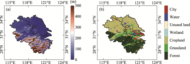
Figure 1 Elevation (a) and land use type (b) from MODIS in 2010 of the Yangtze River Delta

2.2 Remote sensing data

To drive the BEPS and Revised-EC-LUE models, the LAI product of the GLASS dataset (V60) was selected, which is generated from the MODIS-based surface reflectance product using the bidirectional long short-term memory model (Ma and Liang, 2022). Compared with other LAI products, GLASS LAI has higher quality and accuracy and can capture the growth cycle and mutation of vegetation well. The spatial resolution of this dataset is 0.05°, and the temporal resolution is 8 days. Assuming that the LAI remained unchanged for 8 days, the 8-day data were expanded to daily, and the temporal range is 2001-2020. The land use type was from MODIS (MCD12C1). The spatial resolution of this dataset is 0.05°, and the temporal resolution is yearly. The International Geosphere-Biosphere Programme classes were selected, and we aggregated the data into 7 categories (Figure 1b). Data for 2010 was used as the reference.

2.3 Meteorological data

Meteorological data came from ERA5, which is generated based on reanalysis techniques and provides changes in global meteorological elements over decades (Bell et al., 2021). The eastward component of the wind at 10 meters and the northward component of the wind at 10 meters were selected to calculate the horizontal wind speed. We also selected air temperature at 2 meters, dew point temperature at 2 meters, total solar radiation and direct solar radiation. The spatial resolution of wind speed and temperature is 0.1°, the spatial resolution of radiation is 0.25°, and the temporal resolution is hourly. In a small region, the meteorological data are uniform, so it is assumed that the growth environment of vegetation within a 0.1° (0.25°) pixel is similar. Based on this assumption, all data were extended to 0.05° using nearest neighbor resampling, and hourly data were aggregated to daily. VPD was calculated using air temperature and dew point temperature (Yuan et al., 2019). The CO2 concentration was obtained from NOAA’s Earth System Research Laboratory with a temporal resolution of monthly, assuming that the CO2 concentration remains constant on a monthly scale, extending the monthly data to daily data. The temporal range of all data is 2001-2020.

2.4 Solar-induced chlorophyll fluorescence (SIF) data

Considering the uncertainty of the input data and model structure, we selected two SIF datasets (GOSIF and CSIF) to compare with the GPP simulated by the two models. The two SIF datasets are GOSIF upscaled based on the Cubist regression tree model (Li and Xiao, 2019) and CSIF upscaled based on an artificial neural network (Zhang et al., 2018). The spatial resolutions of GOSIF and CSIF are 0.05° and 0.5°, respectively, and the temporal resolution is monthly. The temporal range of the two datasets is 2001-2020.

2.5 DGVM data

Due to the absence of some simulation scenarios and simulated variables, we only selected the GPP simulated by 7 DGVMs (GLM5.0 (Lawrence et al., 2019), ISAM (Meiyappan et al., 2015), ISBA-CTRIP (Delire et al., 2020), JULES-ES (Sellar et al., 2019), LPJ-LUESS (Smith et al., 2014), ORCHIDEEv3 (Vuichard et al., 2019), and SDGVM (Walker et al., 2017)) from TRENDY V9. All models follow the same protocol and use the same forcing data (CO2, climate, LUCC). We used four scenarios: S0 (no forcing change), S1 (only CO2 change), S2 (only CO2 and climate change) and S3 (CO2, climate and LUCC change together). The temporal range used by all models is 2001-2019, and details about DGVM can be found in Friedlingstein et al. (2020). Following the method of Zhu et al. (2016), S1-S0, S2-S1, and S3-S2 were used to evaluate the GPP responses to the CO2 fertilization effect, climate change, and LUCC, respectively.

2.6 BEPS and the Revised-EC-LUE model

BEPS is a diagnostic model driven by remote sensing data (LAI, land use type) and meteorological data (air temperature, VPD, radiation, wind speed). The value of the canopy GPP is the sum of the GPP of the sunlit leaves and shaded leaves. The basic equation is as follows:
$GPP=LA{{I}_{sun}}\times GP{{P}_{sun}}+LA{{I}_{shade}}\times GP{{P}_{shade}}$
where LAIsun and LAIshade represent the LAI of the sunlit leaves and shaded leaves, respectively, and GPPsun and GPPshade represent the GPP per unit area of the sunlit leaf and the shaded leaf, respectively. GPPsun and GPPshade were calculated using the Farquhar model. The Ball-Woodrow-Berry equation was used to simulate stomatal conductance and quantify the effect of CO2 fertilization on GPP (Leuning et al., 1995). The equation and parameters of BEPS were described in detail by Chen et al. (1999, 2012).
The Revised-EC-LUE model considers the effects of direct radiation and diffuse radiation on the canopy and integrates the effects of environmental variables such as CO2 and VPD on GPP. The basic equation is as follows:
$GPP=\left( {{\varepsilon }_{sun}}\times APA{{R}_{sun}}+{{\varepsilon }_{shade}}\times APA{{R}_{shade}} \right)\times {{C}_{s}}\times \text{min}\left( {{T}_{s}},{{W}_{s}} \right)$
where APARsun and APARshade represent the radiation absorbed by the sunlit leaves and shaded leaves, respectively, εsun and εshade represent the light use efficiency of the sunlit leaves and shaded leaves, respectively, and Cs, Ts, and Ws represent the CO2 constraint, temperature constraint, and moisture constraint, respectively. The equation and parameters of the Revised-EC-LUE model were described in detail by Zheng et al. (2020).
Based on remote sensing data and meteorological data, the BEPS and Revised-EC-LUE models were run daily on the 0.05 scale to generate GPP for 2001-2020. For consistency with SIF data and TRENDY data, daily data were aggregated to a monthly scale for analysis.

2.7 Contribution of environmental factors to interannual variation in GPP

To evaluate the contribution of drivers to the interannual variation in GPP, without changing the model parameters, four simulation scenarios were used to drive the BEPS and Revised-EC-LUE models. CO2 concentration remained unchanged from 2001, and other variables changed normally (SS1); LAI remained unchanged from 2001, and other variables changed normally (SS2); climatic conditions (temperature, VPD, radiation) remained unchanged from 2001, and other variables changed normally (SS3); and all variables changed normally (SS4). The sensitivity of each driver to GPP is calculated as follows (Chen et al., 2019b; Zheng et al., 2020):
$GP{{P}_{SS4}}-GP{{P}_{SS1}}={{\beta }_{CO2}}\times \left( CO{{2}_{SS4}}-CO{{2}_{SS1}} \right)+\varepsilon $
$GP{{P}_{SS4}}-GP{{P}_{SS2}}={{\beta }_{LAI}}\times \left( LA{{I}_{SS4}}-LA{{I}_{SS2}} \right)+\varepsilon $
$GP{{P}_{SS4}}-GP{{P}_{SS3}}={{\beta }_{T}}\times \left( {{T}_{SS4}}-{{T}_{SS3}} \right)+$
${{\beta }_{VPD}}\times \left( VP{{D}_{SS4}}-VP{{D}_{SS3}} \right)+{{\beta }_{SRAD}}\times \left( SRA{{D}_{SS4}}-SRA{{D}_{SS3}} \right)+\varepsilon $
where GPPSS1, GPPSS2, GPPSS3, and GPPSS4 are the annual total amount of simulated GPP based on the four scenarios. CO2SS4, LAISS4, TSS4, VPDSS4 and SRADSS4 are the annual means of the CO2 concentration, LAI, temperature, VPD and radiation for 2001-2020, respectively. CO2SS1, LAISS2, TSS3, VPDSS3 and SRADSS3 are the annual means of the CO2 concentration, LAI, temperature, VPD and radiation in 2001, respectively. β is a sensitivity factor, and ε is a random term. The actual contribution of each driver to the interannual variation in GPP is obtained by multiplying the sensitivity of each driver by the variation.

3 Results

3.1 The spatiotemporal characteristics of LAI in the YRD

Similar to the topographical distribution, the LAI in the YRD also showed a gradually decreasing distribution from south to north (Figure 2a). In the southern high-altitude areas, the LAI was generally higher, exceeding 2.5 m2 m-2; however, in the northern plains, the LAI remained only at 1-2 m2 m-2, and in some urban areas, it was even lower. Approximately 85.31% of the YRD showed a positive trend of LAI (greening), and the significantly greening areas were concentrated in the southern part of the YRD, with the trend mostly reaching 0.05 m2 m-2 yr-1. In contrast, LAI showed a coexistence of increase and decrease in the north, especially in some urban areas, and the decrease in LAI was very pronounced (Figure 3b). Figures 3c and 3d show the seasonal variation in the LAI of cropland and natural vegetation (including forests, grasslands and wetlands) in the YRD. Generally, it was high in summer and low in winter, and the LAI of natural vegetation was higher than that of cropland in each month, while the cropland also showed obvious double-high peak characteristics (April and August), possibly due to double cropping in the area.
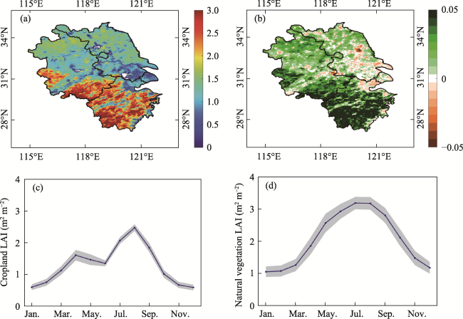
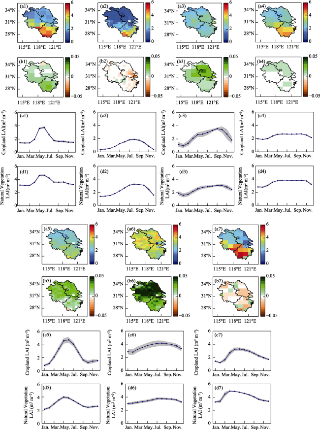
Figure 2 The spatial distribution and seasonal variation in LAI in the Yangtze River Delta from 2001 to 2020. a and b represent the multiyear mean and trend of LAI, c and d represent the LAI seasonal variation in cropland and natural vegetation, the blue line is the mean from 2001 to 2020, and the gray area is the standard deviation.
From 2001 to 2020, the LAI in the YRD showed a significant increasing trend (Figure 3), and the increasing rate reached 2.22 × 10⁻² m2 m-2 yr-1, of which the increasing rate of natural vegetation LAI (3.53×10⁻² m2 m-2 yr-1) was more than twice that of cropland LAI (1.39×10⁻² m2 m-2 yr-1). In addition, the multiyear mean natural vegetation LAI (2.05 ± 0.21 m2 m-2) was significantly higher than that of cropland LAI (1.29 ± 0.09 m2 m-2).
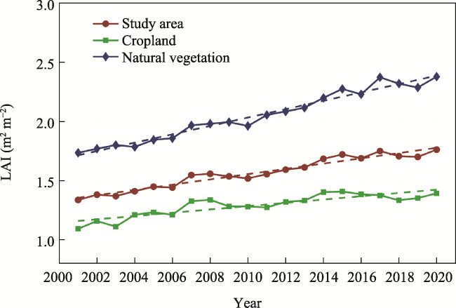
Figure 3 Interannual variation in LAI in the Yangtze River Delta from 2001 to 2020

3.2 The spatiotemporal characteristics of GPP in the YRD

Both the GPP simulated by BEPS and the Revised-EC-LUE model showed a spatial distribution of high in the south and low in the north (Figures 4a and 4e); however, they showed significant differences in the value of the GPP. The GPP simulated by the Revised-EC-LUE model was generally lower, with values below 1000 gC m-2 yr-1 in the northern cropland and only approximately 1500 gC m-2 yr-1 in the southern forest. In contrast, the GPP simulated by BEPS typically reached approximately 1500 gC m-2 yr-1 in northern cropland and over 2000 gC m-2 yr-1 in southern forest.
The GPP simulated by the two models also showed a consistent situation in terms of spatial trend (Figures 4b and 4f). The GPP simulated by BEPS reached 30 gC m-2 yr-2. The GPP simulated by the Revised-EC-LUE model tended to be lower, most of which were below 20 gC m-2 yr-2. Compared with natural vegetation, the difference in GPP simulated by the two models was more reflected in cropland, and the GPP simulated by BEPS was significantly higher than the GPP simulated by the Revised-EC-LUE model in each month (Figures 4c-4d and 4g-4h).
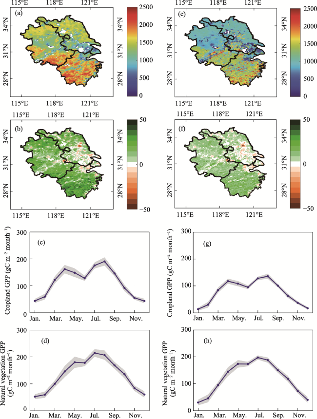
Figure 4 Spatial distribution and seasonal variation in GPP simulated by BEPS and the Revised-EC-LUE model in the Yangtze River Delta. a-d represent the multiyear mean, trend, and seasonal variation in GPP of cropland and natural vegetation simulated by BEPS from 2001 to 2020, e-h represent the multiyear mean, trend, and seasonal variation in GPP of cropland and natural vegetation simulated by the Revised-EC-LUE model from 2001 to 2020, the blue line is the mean from 2001 to 2020, and the gray area is the standard deviation.
Although there were differences in the multiyear mean and trend of GPP, the GPP simulated by the two models consistently captured the signal of double cropping in the YRD, and the GPP consistently showed a significant increasing trend (BEPS: 15.59 gC m-2 yr-2, Revised-EC-LUE model: 7.32 gC m-2 yr-2) (Figure 5); the increasing rate of natural vegetation GPP (BEPS: 19.82 gC m-2 yr-2, Revised-EC-LUE model: 10.44 gC m-2 yr-2) was consistently higher than that of cropland GPP (BEPS: 14.48 gC m-2 yr-2, Revised-EC-LUE model: 5.91 gC m-2 yr-2). At the same time, the multiyear mean of natural vegetation GPP (BEPS: 1586 ± 123 gC m-2 yr-1, Revised-EC-LUE model: 1424 ± 71 gC m-2 yr-1) was consistently higher than that of cropland GPP (BEPS: 1364 ± 97 gC m-2 yr-1, Revised-EC-LUE model: 921 ± 51 gC m-2 yr-1). These spatiotemporal characteristics were identical to those of the LAI.
Figure 5 Interannual variation in GPP simulated by BEPS (a) and the Revised EC-LUE model (b) in the Yangtze River Delta from 2001 to 2020
The spatiotemporal characteristics of the two SIF datasets were further analyzed, and we found that the spatial distribution, spatial trend, and double-high peak characteristics of the two SIF datasets were consistent with the GPP simulated by the two models (Figure S1), and both SIF maintained a significant increasing trend (GOSIF: 1.6×10⁻³ W m−2 μm−1 sr−1, CSIF: 1.7×10⁻³ W m−2 μm−1 sr−1) (Figure S2). Considering that the two SIF datasets are independent of the GPP simulated by the two models and to a certain extent, the SIF is linearly related to the GPP, we consider the GPP simulated by the two models to be reliable (regardless of the value of the simulated GPP).

3.3 The drivers of interannual variation in GPP in the YRD

When all variables changed normally, the trend of GPP simulated by BEPS and the Revised-EC-LUE model from 2001 to 2020 was 5.42 Tg C yr-1 and 2.54 Tg C yr-1, respectively (Figure S3). When the climate factor remained unchanged since 2001, the trend still reached 6.1 Tg C yr-1 and 3.34 Tg C yr-1. When CO2 (LAI) remained unchanged since 2001, the trend of GPP decreased significantly to 3.13 (1.87) Tg C yr-1 and 1.17 (-0.14) Tg C yr-1. The difference indicated that the main drivers of interannual variation in GPP in the YDR were the effect of LAI variation and the CO2 fertilization effect, while the effect of climate change was relatively small.
Sensitivity analysis showed that variations in CO2, LAI, temperature, VPD and radiation all had significant effects on GPP in the YRD (Figure 6). CO2, LAI, temperature and radiation had a positive effect with each increase of one unit (10 ppm, 0.1, 1°C, 10 W); the GPP simulated by BEPS increased by 10.33, 19.31, 6.74, 15.57 Tg C, respectively, and the GPP simulated by the Revised-EC-LUE model increased by 3.02, 12.3, 13.25, 19.85 Tg C, respectively. The increase in VPD led to a decrease in GPP. For every 1 kPa increase in VPD, the GPP simulated by BEPS and the Revised-EC-LUE model decreased by 2.57 Tg C and 26.43 Tg C, respectively. Combined with the actual variations in drivers in the YRD, the increase in LAI (CO2) resulted in an increase in GPP from 2001 to 2020 by 4.29 (2.29) Tg C yr-1 for BEPS and 2.73 (0.67) Tg C yr-1 for the Revised-EC-LUE model. While there was no significant trend in temperature and VPD, its effect on GPP was also relatively limited, and only radiation showed a weak negative effect (-0.73 Tg C yr-1 for BEPS and -0.94 Tg C yr-1 for the Revised-EC-LUE model).
Figure 6 Sensitivity analysis of the drivers of GPP variation in the Yangtze River Delta from 2001 to 2020 (a) and the actual impact of drivers on GPP variation in the Yangtze River Delta (b)

3.4 Reliability of GPP simulated by GDVM in the YRD

GPP simulated by most DGVMs (except for ORCHIDEEv3) maintained the spatial pattern of high in the south and low in the north, which was consistent with the GPP simulated by remote sensing models (Figure 7). ISBA-CTRIP, JULES-ES, LPJ-LUESS, and ORCHIDEEv3 showed increasing trends in GPP, while the other three models showed no significant trend. In addition, the 6 DGVMs except ORCHIDEEv3 could not capture the double cropping characteristics of cropland.
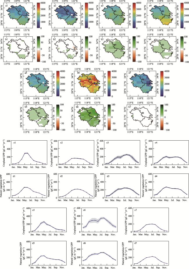
Figure 7 The spatial distribution and seasonal variation in GPP simulated by 7 DGVMs in the Yangtze River Delta. a and b represent the multiyear mean and trend of GPP; c and d represent the seasonal variation in GPP of cropland and natural vegetation, the blue line is the mean from 2001 to 2019, and the gray area is the standard deviation. 1-7 are GLM5.0, ISAM, ISBA-CTRIP, JULES-ES, LPJ-LUESS, ORCHIDEEv3, and SDGVM, respectively.
The multiyear mean GPP simulated by DGVMs in the YRD was between 1.25 × 10³ and 2.76 × 10³ gC m-2 yr-1 (Table 1), which was much higher than that of BEPS (1382 gC m-2 yr-1) and the Revised-EC-LUE model (1083 gC m-2 yr-1); however, in terms of increasing rate, most DGVMs (1.62-33.78 gC m-2 yr-2) were lower than that of BEPS (15.59 gC m-2 yr-2) and the Revised-EC-LUE model (7.32 gC m-2 yr-2). Meanwhile, in only 4 of the 7 DGVMs, the increasing rate of natural vegetation GPP simulated by the model was higher than that of cropland GPP. In addition, we found an incredible result: the multiyear mean cropland GPP simulated by ORCHIDEEv3 (2.85×10³ gC m-2 yr-1) was higher than that of the natural vegetation GPP (2.74×10³ gC m-2 yr-1).
Table 1 Multiyear mean and trend of GPP in the Yangtze River Delta simulated by 7 DGVMs (gC m-2 yr-1 for average and gC m-2 yr-2 for trend)
Study area Cropland Natural vegetation
Average Trend Average Trend Average Trend
CLM5.0 1.48×10³ 4.71* 1.3×103 4.32* 1.7×103 5.25*
ISAM 1.25×10³ 1.85* 1.09×103 0.89 1.5×10³ 3.6*
ISBA-CTRIP 1.79×10³ 13.37* 1.69×103 13.13 1.88×10³ 12.74*
JULES-ES 1.87×10³ 6.87* 1.61×103 6.15 2.19×10³ 7.68*
LPJ-GUESS 1.51×10³ 11.05* 1.36×103 13.61* 1.73×103 8.49*
ORCHIDEEv3 2.76×10³ 33.78* 2.85×103 37.18* 2.74×103 30.43*
SDGVM 1.32×10³ 1.62 1.23×10³ 1.04* 1.47×103 2.73

Note: * indicates p < 0.05.

Table 2 shows the response of GPP to different variables in 7 DGVMs. Not all DGVMs showed that the CO2 fertilization effect contributed the most to GPP variation in the YRD from 2001 to 2019. For example, ISBA_CTRIP and SDGVM showed that climate change was the dominant driver of GPP variation in the YRD, while ORCHIDEEv3 showed that LUCC was the dominant driver. All DGVMs showed that the CO2 fertilization effect had a positive effect on GPP in the YRD (1.15-3.19 Tg C yr-1). However, there were large differences in the response of GPP to climate change and LUCC, especially for LUCC, and the difference between the highest value (ORCHIDEEv3) and the lowest value (SDGVM) was 8.76 Tg C yr-1.
Table 2 The trend of GPP simulated by the 7 DGVMs under different simulation scenarios and the response of GPP to different variables in the Yangtze River Delta (Tg C yr-1)
S0 S1 S2 S3 CO2 Climate LUCC
CLM5.0 0 1.91* 1.98* 1.64* 1.91 0.07 -0.35
ISAM -0.19 1.57* 1.53* 0.64* 1.77* -0.05 -0.88*
ISBA-CTRIP -0.37 1.59 3.73 4.65* 1.97* 2.14 0.92*
JULES-ES -0.38 1.72 1.84 2.39* 2.1* 0.12 0.54
LPJ-GUESS -0.07 1.94* 2.03* 3.84* 2.01* 0.09 1.81*
ORCHIDEEv3 -0.19 3* 4.68* 11.75* 3.19* 1.68* 7.06*
SDGVM -0.92* 0.23 2.27* 0.56 1.15* 2.04* -1.7*

Note: * indicates p < 0.05.

4 Discussion

4.1 The variation in GPP dominated by LAI in the YRD

A variety of methods have been developed to estimate the GPP of terrestrial ecosystems, and these methods can be used to simulate global or regional GPP. However, the spatial and temporal patterns of GPP simulated by different models are usually different (Badgley et al., 2019; Mengistu et al., 2021; Wang et al., 2021). Since there are no available GPP data in the YRD in the public dataset, the simulated GPP cannot be validated by site observations; therefore, we used two models to further reduce the uncertainty of the findings. The BEPS and Revised-EC-LUE models are two representative models that have been widely used in global or regional GPP simulations, and the simulation results are relatively accurate (Feng et al., 2007; Sprintsin et al., 2012; Zheng et al., 2020). In addition, the simulation results of this study were highly consistent with the two independent SIF datasets, which indicates that the simulation results of BEPS and the Revised EC-LUE model are credible in the YRD and can be used for attribution analysis of GPP variation.
As the largest carbon flux in terrestrial ecosystems, the drivers of GPP variation have always been the focus of carbon cycling research. In terms of diurnal variation, GPP is usually controlled by temperature, precipitation and radiation, while in terms of seasonal variation, LAI greatly affects GPP because the impact of meteorological elements on GPP is mostly reflected by LAI. In our study, LAI and GPP simulated by the two models showed obvious consistency in seasonal variation, spatial pattern and characteristics of cropland and natural vegetation. However, in terms of the drivers of interannual variation, the CO2 fertilization effect is considered to be the most important driver of global GPP increase in both free-air CO2 enrichment experiments and model simulations (Ainsworth and Rogers, 2007; Walker et al., 2021). As a substrate for photosynthesis, the increase in CO2 concentration will promote photosynthesis and increase the carbon sequestration capacity of vegetation. Our results also indicate the positive effect of CO2 fertilization on GPP in the YRD, which is consistent with some previous studies (Ainsworth and Rogers, 2007; Walker et al., 2021). Notably, evidence based on remote sensing suggests that the CO2 fertilization effect may have declined in recent years (Wang et al., 2020).
In contrast to previous studies, we found that the LAI variation dominated the interannual variation in GPP in the YRD, and its effect on GPP (4.29 Tg C yr-1 for BEPS and 2.73 Tg C yr-1 for the Revised-EC-LUE model) was much higher than that of the CO2 fertilization effect (2.29 Tg C yr-1 for BEPS and 0.67 Tg C yr-1 for the Revised-EC-LUE model). Generally, LAI variation is affected by various drivers, including LUCC, land management, the CO2 fertilization effect, and climate change. A study by Zhu et al. (2016) showed that the CO2 fertilization effect explained 70% of the global greening trend; however, we noticed that the increasing rate of LAI in the YRD (2.22×10⁻² m2 m-2 yr-1) was much higher than that at the global scale (0.69×10⁻² m2 m-2 yr-1) (Ding et al., 2020). Considering that the CO2 fertilization effect on the global and regional scales is similar, and the temperature and VPD variations in the YRD are not significant, there may be other factors affecting the LAI variation. We searched some statistical indicators of agriculture and forestry in the YRD from the National Bureau of Statistics of China, and we found that land management is also an important factor in the increase in LAI in the YRD (Figure S4). The role of green revolutions such as agricultural mechanization is significant, especially for agricultural areas. From 2001 to 2020, the sown area of crops in the YRD increased by 10%, but the crop yield increased by more than 20%. In addition, large-scale afforestation exists in the YRD. From 2004 to 2020, the forest area increased by 1.07×10⁶ ha. Therefore, we believe that the CO2 fertilization effect and land management jointly led to the LAI variation in the YRD, which further indirectly affected the GPP variation.
In the YRD, the impact of climate change on GPP is relatively small. On the one hand, the impact of climate change on vegetation has been partially included in the LAI variation. On the other hand, climate change is not significant on a relatively short time scale. Limited by the availability of nitrogen deposition datasets, this study did not evaluate the impact of nitrogen deposition on GPP in the YRD, which needs to be considered in future studies. Several recent studies have suggested that nitrogen availability can limit the positive effect of CO2 fertilization on vegetation photosynthesis (He et al., 2017; Wang et al., 2020).
In conclusion, our study highlights the importance of LAI variation to GPP variation in the YRD, and further research is needed to determine whether LAI variation has dominated GPP variation in other areas of the globe with significant greening, such as India or the rest of China.

4.2 Uncertainty of GPP simulated by DGVM

Although the development and improvement of the DGVM is moving forward, studies from global to regional scales have reported uncertainties in carbon fluxes simulated by the DGVM (Seiler et al., 2022). The absence of some key processes and the inability to accurately quantify the complex nonlinear interactions of climate and vegetation may be the underlying cause (Medlyn et al., 2015; Fleischer et al., 2019). As an area with a uniform distribution of vegetation types and a significant role in land management, GPP simulated by remote sensing models in the YRD has some significant characteristics, such as the double-high peak characteristic of cropland GPP, the significantly increasing trend, and differences in natural vegetation GPP and cropland GPP. However, these characteristics cannot be fully captured by any one DGVM, which further emphasizes the uncertainty of the GPP simulated by DGVM at the regional scale.
DGVM mostly estimates GPP based on the Farquhar model and its improved version. When upgrading from the leaf scale to the canopy scale, LAI is an essential variable, so the uncertainty of LAI simulated by DGVM will be further propagated to the estimation results of GPP (Farquhar et al., 1980; von Caemmerer and Farquhar, 1981; Restrepo-Coupe et al., 2017; Murray-Tortarolo et al., 2022). We further verified the spatial pattern and seasonal variation in the LAI simulated by the 7 DGVMs under the S3 scenario. We found that the LAI simulated by DGVM was not consistent with the LAI based on remote sensing observations, whether in terms of spatial mean, spatial trend, or double-cropping of cropland in the area (Figure S5). In addition, similar to the GPP simulated by DGVM, the LAI simulated by DGVM was much higher than the LAI based on remote sensing observations. However, in terms of trend, most DGVMs were lower than LAI based on remote sensing observations (Table S1). Although the DGVM does not have a scenario simulation of the GPP response to LAI, the LAI simulated by the DGVM in the YRD may also dominate (at least to a large extent) the GPP variation. Based on the findings of this study, we believe that the first consideration of DGVM in improving carbon flux should not be the deviation of the model structure but the accuracy of the input data (i.e., the simulated LAI). This is also supported by Seiler et al.’s evaluation of the various simulated variables of DGVM, who found that the LAI simulated by DGVM has a high positive bias compared to the satellite observation (Seiler et al., 2022).
Some methods may improve LAI/GPP simulated by DGVM. One of the most typical is the inclusion of critical processes. Using statistical methods based on remote sensing, the extensive impacts of land management on vegetation from global to regional scales have been further identified and emphasized (Chen et al., 2019a; Chen et al., 2022a; 2022b). However, due to the complexity of the management process and the lack of management data, although some DGVMs have made efforts, the characterization of the management process by the model remains unfortunate, which may require more theoretical and mechanistic research. In contrast, the input data significantly improved the simulation results of DGVM, and some studies have found that the bias of LUCC may increase the uncertainty of simulation results. Yu et al. (2022) used reconstructed LUCC in China to drive a dynamic terrestrial ecosystem model and found that the main contribution of China’s terrestrial ecosystem carbon sink from 2001 to 2019 came from forest restoration (44%), highlighting the positive effect of land management on the terrestrial carbon budget. A study by Zhou et al. (2022) also showed that incorrect LUCC data in Eastern Europe led to a serious underestimation of the carbon sink in this area. Therefore, in the YRD, the lack of land management or bias of LUCC may be the potential causes for the large deviation of LAI/GPP simulation in the DGVM.

5 Conclusion

Based on the BEPS and Revised-EC-LUE models, we found that the GPP showed a significant increasing trend from 2001 to 2020 in the YRD (15.59 gC m-2 yr-2 for BEPS and 7.32 gC m-2 yr-2 for the Revised-EC-LUE model). The multiyear mean and increasing rate of the natural vegetation GPP were higher than those of the cropland GPP. In addition, the cropland GPP in this area had obvious double-high peak characteristics. These characteristics were consistent with the LAI, and the two SIF datasets also showed the same results. Simulation results based on different scenarios showed that the effect of LAI variation determined the interannual variation in GPP in the YRD, and its effect (4.29 Tg C yr-1 for BEPS and 2.73 Tg C yr-1 for the Revised-EC-LUE model) was higher than the CO2 fertilization effect (2.29 Tg C yr-1 for BEPS and 0.67 Tg C yr-1 for the Revised-EC-LUE model). Therefore, we believe that LAI has dominated the GPP variation in the YRD, including spatial and temporal variation. However, none of the 7 DGVMs could capture these significant characteristics of GPP in this area, which might be caused by the deviation of LAI simulation. Our results emphasize the importance of LAI in GPP simulation. It is worth noting that the LAI variation is also driven by various factors, such as the CO2 fertilization effect and land management.

Supplementary figures and tables

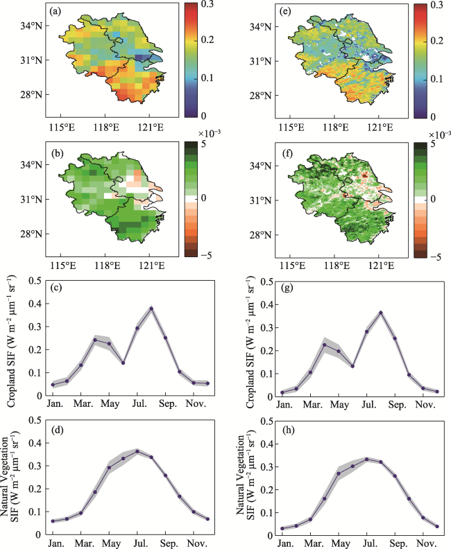
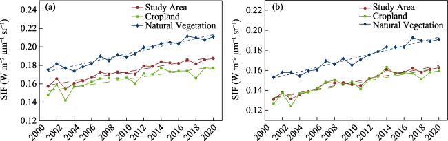
Figure S1 Spatial distribution and seasonal variation in CSIF and GOSIF. a-d represent the multiyear mean, trend, and seasonal variation in cropland and natural vegetation of CSIF from 2001 to 2020, e-h represent the multiyear mean, trend, seasonal variation in cropland and natural vegetation of GOSIF from 2001 to 2020, the blue line is the mean from 2001 to 2020, and the gray area is the standard deviation.
Figure S2 Interannual variation in CSIF (a) and GOSIF (b) from 2001 to 2020
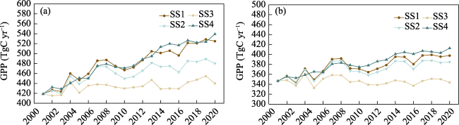
Figure S3 Variation in GPP in the YRD from 2001 to 2020 simulated by BEPS (a) and the Revised-EC-LUE model (b) under different simulation scenarios
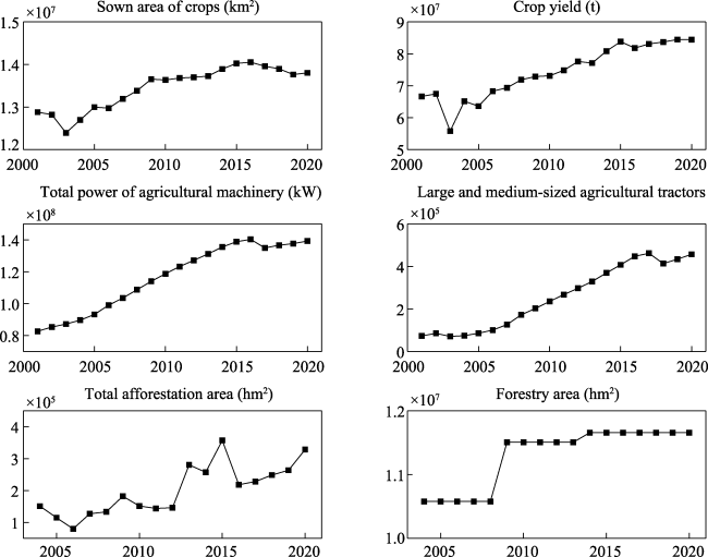
Figure S4 Variations in some agriculture and forestry in the Yangtze River Delta. The temporal range of agriculture is 2001-2020, and the time range of forestry is 2004-2020
Figure S5 The spatial distribution and seasonal variation in LAI simulated by 7 DGVMs in the Yangtze River Delta. a and b represent the multiyear mean and trend of LAI, c and d represent the seasonal variation in LAI of cropland and natural vegetation, the blue line is the mean from 2001 to 2019, and the gray area is the standard deviation. 1-7 are GLM5.0, ISAM, ISBA-CTRIP, JULES-ES, LPJ-LUESS, ORCHIDEEv3, and SDGVM, respectively.
Table S1 Multiyear mean and trend of LAI simulated by 7 DGVMs in the Yangtze River Delta (m2 m-2 for average and m2 m-2 yr-1 for trend)
Study area Cropland Natural vegetation
Average Trend Average Trend Average Trend
CLM5.0 2.76 7.92×10-3* 2.02 4.4×10⁻³ 3.65 12.19×10⁻³*
ISAM 1.62 -2.6×10⁻³ 1.09 -2.7×10⁻³ 2.3 -1.37×10⁻³
ISBA-CTRIP 2.46 13.45×10⁻³ 2.39 14.47×10⁻³ 2.5 11.15×10⁻³
JULES-ES 2.89 3.2×10-3* 2.42 3.76×10-3* 3.48 2.6×10⁻³*
LPJ-GUESS 2.63 16.53×10-3* 2.41 21.39×10-3* 2.96 11.22×10⁻³*
ORCHIDEEv3 3.49 36.34×10-3* 3.63 43.04×10-3* 3.45 29.52×10⁻³*
SDGVM 3.1 -3.12×10⁻³ 2.36 -2.85×10⁻³ 4.1 -2.88×10⁻³

Note: * indicates p < 0.05.

[1]
Ainsworth E A, Rogers A, 2007. The response of photosynthesis and stomatal conductance to rising CO2: Mechanisms and environmental interactions. Plant Cell and Environment, 30(3): 258-270.

DOI

[2]
Badgley G, Anderegg L D L, Berry J A et al., 2019. Terrestrial gross primary production: Using NIRV to scale from site to globe. Global Change Biology, 25(11): 3731-3740.

DOI

[3]
Badgley G, Field C B, Berry J A, 2017. Canopy near-infrared reflectance and terrestrial photosynthesis. Science Advances, 3(3): e1602244.

DOI

[4]
Bell B, Hersbach H, Simmons A et al., 2021. The ERA5 global reanalysis: Preliminary extension to 1950. Quarterly Journal of the Royal Meteorological Society, 147(741): 4186-4227.

DOI

[5]
Chen C, Park T, Wang X et al., 2019a. China and India lead in greening of the world through land-use management. Nature Sustainability, 2(2): 122-129.

DOI

[6]
Chen J M, Ju W, Ciais P et al., 2019b. Vegetation structural change since 1981 significantly enhanced the terrestrial carbon sink. Nature Communications, 10(1): 4259.

DOI

[7]
Chen J M, Liu J, Cihlar J et al., 1999. Daily canopy photosynthesis model through temporal and spatial scaling for remote sensing applications. Ecological Modelling, 124(2/3): 99-119.

[8]
Chen J M, Mo G, Pisek J et al., 2012. Effects of foliage clumping on the estimation of global terrestrial gross primary productivity. Global Biogeochemical Cycles, 26(1): GB1019.

[9]
Chen T, Dolman H, Sun Z et al., 2022a. Land management explains the contrasting greening pattern across China-Russia border based on paired land use experiment approach. Journal of Geophysical Research: Biogeosciences, 127(6): e2021JG006659.

[10]
Chen T, Guo R, Yan Q et al., 2022b. Land management contributes significantly to observed vegetation browning in Syria during 2001-2018. Biogeosciences, 19(5): 1515-1525.

DOI

[11]
Chen X, Chen T, Shu Y et al., 2021. A framework to assess the potential uncertainties of three FPAR products. Journal of Geophysical Research: Biogeosciences, 126(10): e2021JG006320.

[12]
Chu H, Luo X, Ouyang Z et al., 2021. Representativeness of eddy-covariance flux footprints for areas surrounding AmeriFlux sites. Agricultural and Forest Meteorology, 301: 108350.

[13]
Delire C, Seferian R, Decharme B et al., 2020. The global land carbon cycle simulated with ISBA-CTRIP: Improvements over the last decade. Journal of Advances in Modeling Earth Systems, 12(9): e2019MS001886.

[14]
Ding Z, Peng J, Qiu S et al., 2020. Nearly half of global vegetated area experienced inconsistent vegetation growth in terms of greenness, cover, and productivity. Earths Future, 8(10): e2020EF001618.

[15]
Farquhar G D, von Caemmerer S, Berry J A, 1980. A biochemical model of photosynthetic CO2 assimilation in leaves of C3 species. Planta, 149(1): 78-90.

DOI PMID

[16]
Feng X, Liu G, Chen J M et al., 2007. Net primary productivity of China’s terrestrial ecosystems from a process model driven by remote sensing. Journal of Environmental Management, 85(3): 563-573.

PMID

[17]
Fleischer K, Rammig A, De Kauwe M G et al., 2019. Amazon forest response to CO2 fertilization dependent on plant phosphorus acquisition. Nature Geoscience, 12(9): 736.

DOI

[18]
Friedlingstein P, O’Sullivan M, Jones M W et al., 2020. Global Carbon Budget 2020. Earth System Science Data, 12(4): 3269-3340.

DOI

[19]
He L, Chen J M, Croft H et al., 2017. Nitrogen availability dampens the positive impacts of CO2 fertilization on terrestrial ecosystem carbon and water cycles. Geophysical Research Letters, 44(22): 11590-11600.

DOI

[20]
Houghton R A, 2020. Terrestrial fluxes of carbon in GCP carbon budgets. Global Change Biology, 26(5): 3006-3014.

DOI PMID

[21]
Jung M, Schwalm C, Migliavacca M et al., 2020. Scaling carbon fluxes from eddy covariance sites to globe: Synthesis and evaluation of the FLUXCOM approach. Biogeosciences, 17(5): 1343-1365.

DOI

[22]
Keenan T F, Williams C A, 2018. The terrestrial carbon sink. Annual Review of Environment and Resources, 43: 219-243.

DOI

[23]
Lawrence D M, Fisher R A, Koven C D et al., 2019. The community land model Version 5: Description of new features, benchmarking, and impact of forcing uncertainty. Journal of Advances in Modeling Earth Systems, 11(12): 4245-4287.

DOI

[24]
Leuning R, Kelliher F M, De Pury D G G et al., 1995. Leaf nitrogen, photosynthesis, conductance and transpiration: Scaling from leaves to canopies. Plant, Cell & Environment, 18(10): 1183-1200.

[25]
Li X, Xiao J, 2019. A global, 0.05-degree product of solar-induced chlorophyll fluorescence derived from OCO-2, MODIS, and reanalysis data. Remote Sensing, 11(5): 517.

DOI

[26]
Ma H, Liang S, 2022. Development of the GLASS 250-m leaf area index product (version 6) from MODIS data using the bidirectional LSTM deep learning model. Remote Sensing of Environment, 273: 112985.

DOI

[27]
Medlyn B E, Zaehle S, De Kauwe M G et al., 2015. Using ecosystem experiments to improve vegetation models. Nature Climate Change, 5(6): 528-534.

DOI

[28]
Meiyappan P, Jain A K, House J I, 2015. Increased influence of nitrogen limitation on CO2 emissions from future land use and land use change. Global Biogeochemical Cycles, 29(9): 1524-1548.

DOI

[29]
Mengistu A G, Tsidu G M, Koren G et al., 2021. Sun-induced fluorescence and near-infrared reflectance of vegetation track the seasonal dynamics of gross primary production over Africa. Biogeosciences, 18(9): 2843-2857.

DOI

[30]
Murray-Tortarolo G, Poulter B, Vargas R et al., 2022. A process-model perspective on recent changes in the carbon cycle of North America. Journal of Geophysical Research: Biogeosciences, 127(9) e2022JG006904.

[31]
Pei Y, Dong J, Zhang Y et al., 2022. Evolution of light use efficiency models: Improvement, uncertainties, and implications. Agricultural and Forest Meteorology, 317: 108905.

DOI

[32]
Piao S, Wang X, Wang K et al., 2020. Interannual variation of terrestrial carbon cycle: Issues and perspectives. Global Change Biology, 26(1): 300-318.

DOI PMID

[33]
Restrepo-Coupe N, Levine N M, Christoffersen B O et al., 2017. Do dynamic global vegetation models capture the seasonality of carbon fluxes in the Amazon basin? A data-model intercomparison. Global Change Biology, 23(1): 191-208.

DOI PMID

[34]
Seiler C, Melton J R, Arora V K et al., 2022. Are terrestrial biosphere models fit for simulating the global land carbon sink? Journal of Advances in Modeling Earth Systems, 14(5): e2021MS002946.

[35]
Sellar A A, Jones C G, Mulcahy J P et al., 2019. UKESM1: Description and evaluation of the UK earth system model. Journal of Advances in Modeling Earth Systems, 11(12): 4513-4558.

DOI

[36]
Smith B, Warlind D, Arneth A et al., 2014. Implications of incorporating N cycling and N limitations on primary production in an individual-based dynamic vegetation model. Biogeosciences, 11(7): 2027-2054.

DOI

[37]
Sprintsin M, Chen J M, Desai A et al., 2012. Evaluation of leaf-to-canopy upscaling methodologies against carbon flux data in North America. Journal of Geophysical Research: Biogeosciences, 117(G1): G01023.

[38]
Sun Z, Wang X, Zhang X et al., 2019. Evaluating and comparing remote sensing terrestrial GPP models for their response to climate variability and CO2 trends. Science of the Total Environment, 668: 696-713.

DOI

[39]
von Caemmerer S, Farquhar G D, 1981. Some relationships between the biochemistry of photosynthesis and the gas exchange of leaves. Planta, 153(4): 376-387.

DOI PMID

[40]
Vuichard N, Messina P, Luyssaert S et al., 2019. Accounting for carbon and nitrogen interactions in the global terrestrial ecosystem model ORCHIDEE (trunk version, rev 4999): Multi-scale evaluation of gross primary production. Geoscientific Model Development, 12(11): 4751-4779.

DOI

[41]
Walker A P, De Kauwe M G, Bastos A et al., 2021. Integrating the evidence for a terrestrial carbon sink caused by increasing atmospheric CO2. New Phytologist, 229(5): 2413-2445.

DOI

[42]
Walker A P, Quaife T, van Bodegom P M et al., 2017. The impact of alternative trait-scaling hypotheses for the maximum photosynthetic carboxylation rate (V-cmax) on global gross primary production. New Phytologist, 215(4): 1370-1386.

DOI

[43]
Wang S, Zhang Y, Ju W et al., 2020. Recent global decline of CO2 fertilization effects on vegetation photosynthesis. Science, 370(6522): 1295.

DOI

[44]
Wang Z, Liu S, Wang Y-P et al., 2021. Tighten the bolts and nuts on GPP estimations from sites to the globe: An assessment of remote sensing based LUE models and supporting data fields. Remote Sensing, 13(2): 168.

DOI

[45]
Yu Z, Ciais P, Piao S et al., 2022. Forest expansion dominates China’s land carbon sink since 1980. Nature Communications, 13(1): 5374.

DOI

[46]
Yuan W, Cai W, Xia J et al., 2014. Global comparison of light use efficiency models for simulating terrestrial vegetation gross primary production based on the La Thuile database. Agricultural and Forest Meteorology, 192: 108-120.

[47]
Yuan W, Zheng Y, Piao S et al., 2019. Increased atmospheric vapor pressure deficit reduces global vegetation growth. Science Advances, 5(8): eaax1396.

DOI

[48]
Yue X, Unger N, 2015. The Yale Interactive terrestrial Biosphere model version 1.0: Description, evaluation and implementation into NASA GISS ModelE2. Geoscientific Model Development, 8(8): 2399-2417.

DOI

[49]
Zhang Y, Joiner J, Alemohammad S H et al., 2018. A global spatially contiguous solar-induced fluorescence (CSIF) dataset using neural networks. Biogeosciences, 15(19): 5779-5800.

DOI

[50]
Zhao M, Running S W, 2010. Drought-induced reduction in global terrestrial net primary production from 2000 through 2009. Science, 329(5994): 940-943.

DOI PMID

[51]
Zheng Y, Shen R, Wang Y et al., 2020. Improved estimate of global gross primary production for reproducing its long-term variation, 1982-2017. Earth System Science Data, 12(4): 2725-2746.

DOI

[52]
Zheng Y, Zhang L, Xiao J et al., 2018. Sources of uncertainty in gross primary productivity simulated by light use efficiency models: Model structure, parameters, input data, and spatial resolution. Agricultural and Forest Meteorology, 263: 242-257.

DOI

[53]
Zhou S, Chen T, Zeng N et al., 2022. The impact of cropland abandonment of post-Soviet countries on the terrestrial carbon cycle based on optimizing the cropland distribution map. Biology, 11(5): 620.

DOI

[54]
Zhu Z, Piao S, Myneni R B et al., 2016. Greening of the Earth and its drivers. Nature Climate Change, 6(8): 791-795.

DOI

Outlines

/