Special Issue: Human-environment interactions and Ecosystems

Estimation of maize yield incorporating the synergistic effect of climatic and land use change in Jilin, China

  • WEN Xinyuan , 1 ,
  • LIU Dianfeng , 1, 2, * ,
  • QIU Mingli 1 ,
  • WANG Yinjie 1 ,
  • NIU Jiqiang 3 ,
  • LIU Yaolin 1
Expand
  • 1. School of Resources and Environmental Sciences, Wuhan University, Wuhan 400072, China
  • 2. Key Laboratory of Digital Cartography and Land Information Application Engineering, Ministry of Natural Resources, Wuhan 430072, China
  • 3. Key Laboratory for Synergistic Prevention of Water and Soil Environmental Pollution, Xinyang Normal University, Xinyang 464000, Henan, China
* Liu Dianfeng (1985-), Professor, specialized in land use optimization and simulation. E-mail:

Wen Xinyuan (1999-), Master Candidate, specialized in land use change and sustainable development. E-mail:

Received date: 2022-11-30

  Accepted date: 2023-05-06

  Online published: 2023-08-29

Supported by

National Natural Science Foundation of China(42171414)

National Natural Science Foundation of China(41771429)

The Open Fund of Key Laboratory for Synergistic Prevention of Water and Soil Environmental Pollution(KLSPWSEP-A02)

Abstract

Yield forecasting can give early warning of food risks and provide solid support for food security planning. Climate change and land use change have direct influence on regional yield and planting area of maize, but few studies have examined their synergistic impact on maize production. In this study, we propose an analysis framework based on the integration of system dynamic (SD), future land use simulation (FLUS) and a statistical crop model to predict future maize yield variation in response to climate change and land use change in a phaeozem region of central Jilin province, China. The results show that the cultivated land is likely to reduce by 862.84 km2 from 2030 to 2050. Nevertheless, the total maize yield is expected to increase under all four RCP scenarios due to the promotion of per hectare maize yield. Among the scenarios, RCP4.5 is the most beneficial to maize production, with a doubled total yield in 2050. Notably, the yield gap between different counties will be further widened, which necessitates the differentiated policies of agricultural production and farmland protection, e.g., strengthening cultivated land protection and crop management in low-yield areas, and taking adaptation and mitigation measures to coordinate climate change and production.

Cite this article

WEN Xinyuan , LIU Dianfeng , QIU Mingli , WANG Yinjie , NIU Jiqiang , LIU Yaolin . Estimation of maize yield incorporating the synergistic effect of climatic and land use change in Jilin, China[J]. Journal of Geographical Sciences, 2023 , 33(8) : 1725 -1746 . DOI: 10.1007/s11442-023-2150-6

1 Introduction

Agriculture is a crucial sector that plays a vital role in ensuring food security, reducing poverty, and promoting sustainable development (Loboguerrero et al., 2019). However, with the remarkable growth of the global population, agricultural production has faced significant challenges in meeting the increasing demand for food and accommodating the varying dietary structure of human beings. Moreover, farmland loss and degradation caused by urban expansion and economic development have further exacerbated this situation (Vermeulen et al., 2012). In this context, forecasting food production can provide an early warning of food risk and support agricultural land use activities and corresponding policy-making.
Crop yield prediction methods can be broadly categorized into statistical models and process-based models. Traditional statistical models such as linear and nonlinear regression analyses, and their integration with principal component analysis, have been widely employed to forecast seasonal variations in crop yield (Shi et al., 2013). More recently, machine learning approaches, e.g., random forest, XGBoost, long-short-term memory (LSTM), and convolutional neural network (CNN), have gained more attention due to their ability to describe complex relationships between crop production and driving forces (Hengl et al., 2017; Poornima et al., 2019; Yang et al., 2019; Zhong et al., 2019; Kang et al., 2020; Leng et al., 2020; Sakamoto, 2020). These statistical models are relatively easy to construct and apply, requiring only historical data on the relationship between crop yield and agrometeorological variables, such as average temperature difference, daily relative humidity changes, and sunshine hours, as well as remote sensing-based variables (Camberlin et al., 1999; Giri et al., 2017; Sharma et al., 2017; Banakara et al., 2019), such as the normalized difference vegetation index (Peralta et al., 2016),vegetation condition index (Kowalik et al., 2014), and vegetation health index (Wang et al., 2010). Statistical models are generally robust to noise and outliers, making them useful for analyzing large datasets, and they can be used across a wide range of crops and environments, making them a versatile tool for yield prediction (Urban et al., 2012). However, these models lack the ability to explicitly incorporate the underlying mechanisms of crop growth and identify causal relationships between environmental factors and crop yield.
Process-based crop models employ integrated mathematical methods to describe crop growth status driven by climate, nutrient and water cycling, soil properties, and agricultural management practices (Basso et al., 2016; Rao et al., 2022). These models, including Crop Environment Resource Synthesis (CERES), WOrld FOod STudies (WOFOST), Soil Water Atmosphere Plant Model (SWAP), Environmental Analysis and Remote Sensing (EARS), and the Crop Growth Simulation algorithm (EARS-CGS), have been applied to predict the yield of various crops such as maize, wheat, barley, and millet (Rojas, 2007; Manatsa et al., 2011; Tripathy et al., 2013). They are based on a detailed understanding of the underlying biological, physical, and chemical processes that drive crop growth and yield and can identify causal relationships between environmental factors and crop yield. However, process-based models also suffer from some limitations due to their complex parameters and data requirements (Kolotii et al., 2015). By comparing the strengths and limitations of the two types of models, this study adjusted a statistical model to predict the maize yield per hectare rather than using a process-based crop model due to the large scale of the study area.
Integrating land use change analysis with statistical crop yield models is crucial for accurate yield forecasts (Vancutsem et al., 2013). By using land use simulation models such as cellular automata, changes in agricultural land use patterns and quantity can be projected, allowing for the incorporation of land use change effects into crop yield estimations (Liu et al., 2017; Akpoti et al., 2019). These models can also incorporate complex approaches like neural networks, multiagent systems, and multinomial logistic regression for better simulation performance (Basse et al., 2014; Mustafa et al., 2018). Furthermore, numerous driving factors, such as urbanization, agricultural machinery advancement, and population economic growth, can also be incorporated into maize yields, making the model framework more realistic (Yu et al., 2020; Abate et al., 2021). However, previous studies did not consider the combined response of maize yields to climate change and future changes in maize acreage (Basso et al., 2019). To address this gap, this study developed a generic framework for spatially explicit maize yield forecasting. The framework integrated a statistical crop yield model with a spatial land use simulation model considering various driving factors such as the economy, technology, agricultural investment, population growth, and climate change. Moreover, we devised four future simulation scenarios based on representative concentration pathways (RCPs) to incorporate crop yields into the complex system of human-nature interactions.
Our study was conducted in the phaeozem region of central Jilin province, China, which is part of the Black Soil Region in Northeast China (NEC). NEC is an important food base and one of the most sensitive areas to climate change in China. Some studies predicted that future maize yields would decrease in NEC (Lin et al., 2015; Jiang et al., 2021; Li et al., 2022), while others suggested that future climate change will benefit NEC and enhance maize yields (Pu et al., 2020; Zhang et al., 2023). Therefore, more experimental evidence is needed to reduce uncertainty about the response of maize yields in NEC to socioeconomic development and climate change. As a priority area for agricultural modernization and black soil conservation in China, the study area requires a more detailed policy design. Our study contributes to providing more comprehensive policy recommendations for ensuring food security and sustainable regional development in this area.

2 Materials and methods

2.1 Study area

A phaeozem region in central Jilin province of China was selected as the study area, and it comprises Changchun, Jilin, Siping, Liaoyuan, and Tonghua cities (Figure 1). This region is located in one of the major golden maize belts in the world, and plays an irreplaceable role in national food security as one of the primary grain production bases and commodity grain export bases in China (Asseng et al., 2013; Li et al., 2020; Gao et al., 2023). To eliminate the effect of irrigation on crop yield, our research focused on the rain-fed maize system in the region (Urban et al., 2012). The region features a short maize-growing season from May to September (Yang et al., 2007; Feng et al., 2021). Over the past 50 years, the average annual temperature has risen significantly by 0.38°C per decade, precipitation has decreased slightly. As a result, droughts and floods have become more frequent, posing a direct threat to maize production (Grassini et al., 2009; Yin et al., 2016). Furthermore, climate change has also indirectly affected land use (Pan et al., 2020; Yang et al., 2020). Therefore, it is necessary to assess the future impact of climate change and land use change on maize yields to support agricultural decision-making.
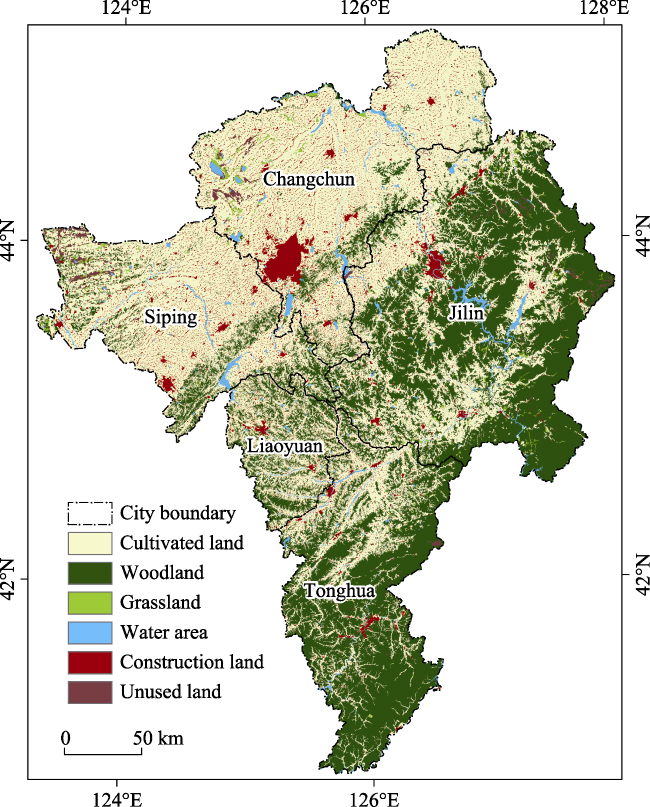
Figure 1 Location of the central Jilin province of China (background: empirical land use map in 2015)

2.2 Data source

The data in this study include climate data, land use maps, socio-economic data, the spatial distribution of population density, the digital elevation model (DEM), road networks, and administrative boundaries (Table 1). Future climate data on precipitation and surface tem-peratures were obtained from WDCC (Knutti, 2014), which were generated by the Beijing Climate Center Climate System Model version 1.1 m (BCC_CSM1.1 m) and has a horizontal resolution of T106 (1.125°×1.125°) (Wu et al., 2010; Liu et al., 2021). These data have been widely used to explore maize, wheat, and other grain planting systems in northeast China (He et al., 2018; Gao et al., 2020). A time series of historical climate data were also down- loaded from the China Meteorological Data Network (http://data.cma.cn).
Table 1 Data and sources
Data Data type Original spatial resolution Temporal coverage Data source
Expenditure and production value of agriculture, forestry, animal husbandry and fishery Excel N/A 2000-2015 Jilin Province Statistical Yearbook
Total mechanical power, total grain production
The proportion of urban population, total urban and rural population
Science and technology expenditure
County-level maize yield data
Historical climate data 2000-2015 http://data.cma.cn/
Annual precipitation and annual average
temperature
NetCDF 1.125° 2006-2100 https://doi.org/10.1594/WDCC/ETHr2
Land use map TIFF 30 m 2000-2015 http://data.casearth.cn/
Spatial distribution of GDP 1 km 2000, 2015 http://www.resdc.cn/
Spatial distribution of population density
DEM 30 m
Road network shapefile N/A https://www.openstreetmap.org/
Administrative boundary 2015 http://www.resdc.cn/
Empirical land use maps in 2000, 2005, 2010, and 2015 were derived from the Chinese Academy of Sciences (CAS; http://www.resdc.cn), and categorized into six types: cultivated land, woodland, grassland, construction land, unused land, and water area (Ning et al., 2018). Socio-economic data, including urban/rural population, GDP, agriculture production, forestry, animal husbandry, and fishery, were obtained from the Statistical Yearbook of Jilin Province (2000-2015). Geographic information data, including DEM, administrative boundaries, roads, and railways, were derived from the Chinese Academy of Sciences database (http://www.resdc.cn/DOI). All spatial data were converted into raster maps at a spatial res-olution of 30m using the ArcGIS 10.5 platform.

3 Methods

3.1 Integrated assessment framework

We proposed an analytical framework to examine the effect of climate change and land use changes on regional maize yield based on the integration of system dynamics (SD), cellular automata (CA), and a statistical maize yield model (Figure 2). SD projects land use demands from a top-down perspective, based on socio-economic development and policy planning. CA simulates spatial land use patterns from a bottom-up perspective, allowing us to predict land use changes in the study area from 2015 to 2050. The integration of SD and CA provides a comprehensive approach to forecasting future land use patterns. Next, a statistical maize yield model was incorporated to predict maize yield per hectare under the influence of temperature, precipitation, agricultural technology, and sunshine hours in four Representative Concentration Pathways (RCPs). This model considered multiple driving factors to accurately estimate per unit maize yield. Then, total maize yields under different scenarios were assessed by multiplying the simulated maize planting area and the predicted maize yield per hectare and compared for two time periods of 2011-2030 and 2031-2050. With this framework, we can examine the impact of climate change and socio-economic development on regional maize yield in a comprehensive manner.
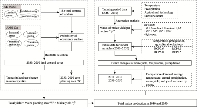
Figure 2 The analytical framework for maize yield prediction

3.2 Future climate scenario design

To examine the impact of climate change and land use changes on regional maize yield, we developed future scenarios based on four Representative Concentration Pathways (RCPs) described in CMIP5, a standard experiment protocol that defines a series of coupled atmos-phere-ocean general circulation models developed by Climate Modeling Groups,World Climate Research Project (WCRP), and International Geosphere-Biosphere Project (IGBP) (Kriegler et al., 2014; O'Neill et al., 2014; van Vuuren et al., 2014; Pan et al., 2020). The four RCPs represent radiative forcing levels of 2.6, 4.5, 6.0, and 8.5 W/m2 by 2100. Each RCP pathway describes a range of climatic and socio-economic characteristics related to different levels of carbon emissions (van Vuuren et al., 2014), such as average temperature and precipitation during the growing season (Figure A1), and the promotion of agricultural mechanization (Rotz et al., 2019). Annual average temperature and annual precipitation under four RCPs were set according to historical and projected climate datasets. The growth rates of agricultural technology under four RCPs were determined based on the actual development of Jilin province and previous research (Huang et al., 2020; Yang et al., 2020) (Table 2).
Table 2 The growth rate of agriculture technology
Scenarios Growth rate
RCP2.6 Level High
Growth rate +7%
RCP4.5 Level Relatively high
Growth rate +5%
RCP6.0 Level Moderate
Growth rate +3%
RCP8.5 Level Low
Growth rate 0

3.3 Projection of future land use demand

The prediction of maize planting areas consists of two main steps: land use demand projection and spatial pattern allocation. In the first step, future land use demands were projected using the system dynamic (SD) model. The SD model enables us to simulate the complex evolution process of the land system by considering feedback and interactions between different system elements (Akhtar et al., 2013).
The SD model in this study comprises three sections: population, social economy, and land use (Figure 3). The population section accounts for changes in urban and rural populations related to socio-economic development and land use demands for urban and rural settlements, as well as agricultural production. The socio-economic section considers the effect of agricultural technology development and fixed asset investment change on agriculture, forestry, and fishing production. The land use section illustrates land use conversions and their driving forces in terms of population, socio-economic development, and interaction among various land use types (Liu et al., 2017). For example, cultivated land may expand due to a series of farmland supplementation measures, e.g., the consolidation of rural settlements and the reclamation of wild grassland, and will decline because of farmland reforestation and urban encroachment. The interaction and feedback among the three sections are defined through regression methods. The SD model covers the time period from 2011 to 2050, with a yearly time step. The outputs of SD are used to constrain land use quantities in the process of spatial land use pattern allocation (see Table A3 for detailed information).
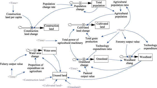
Figure 3 Interaction and feedback relationships in the system dynamic model

3.4 Allocation of spatial land use pattern

The spatial allocation of land use was conducted using the FLUS model based on the land use demand projections from SD. FLUS consists of two modules (Liu et al., 2017): (1) estimating the occurrence probability of each land use type on a specific grid unit based on a three-layer artificial neural network (ANN); (2) determining the land use type of each grid cell based on the cellular automata approach. Specifically, a three-layer ANN was trained using empirical land use data and a set of driving factors that combine socio-economic and natural effects, including population density, GDP, elevation, slope, aspect, distance to main highways, distance to primary railways, distance to rivers, and distance to cities (Yang et al., 2020). CA calculates the combined probability of a specific land use type on each grid cell based on the product of the occurrence probability, land use conversion cost, and coefficients of spatial neighborhood effect and land use inertia (Li et al., 2017), and then assigns the suitable land use type to each grid cell using the roulette selection method (Pan et al., 2020). For detailed model descriptions and parameterizations, please refer to Yang et al. (2020).

3.5 Estimation of maize yield per hectare

Maize yield per hectare was estimated using a regression analysis based on historical data of maize production from 2000 to 2015. Independent variables were selected based on county-level differences, socio-economic development, and physical conditions that are essential for photosynthesis and plant growth. These variables included the mean and squared of temperature and precipitation in the growing season (Lobell et al., 2011; Urban et al., 2012), the total power of agricultural machinery, and sunshine hours (Murchie et al., 2011). To account for the non-linear relationship between climate variables and maize yields and moderately/strongly skewed distribution of maize yields (Huang et al., 2021), the logarithm of the maize yield rather than the yield per se was used as the dependent variable. The quadratic function has been shown promising in simulating dynamic relationships between climate conditions and maize yield (Grassini et al., 2009; Lobell et al., 2010). The regression model for estimating maize yield per unit can be expressed as follows:
$\log \left( {\hat{y}} \right)={{\beta }_{0}}+{{\beta }_{1}}machine+{{\beta }_{2}}machin{{e}^{2}}+{{\beta }_{3}}T+{{\beta }_{4}}{{T}^{2}}+{{\beta }_{5}}P+{{\beta }_{6}}{{P}^{2}}+{{\beta }_{7}}SH+\sum {{\beta }_{i}}count{{y}_{i}}$
where T, P, and SH represent temperature, precipitation, and sunshine hours during the growing season from May to September. county is a dummy variable to capture the spatially heterogeneous influence of physical and socio-economic factors at the county level, such as soil quality and agronomic. machine accounts for an improvement in agricultural mechanization. Square terms of independent variables denote a certain degree of nonlinearity (see Text A1 and Table A1 for detailed parameters).
Moreover, changes in the average maize yield are often accompanied by changes in its variance. The variance of the yield per hectare can serve as a measure of the stability of inter-annual maize production, which is crucial for maintaining stable incomes for farmers and ensuring regional food security. The yield variance can be calculated in the following:
$\begin{align} & Var\left( y \right)={{\left( E\left[ \log \left( {\hat{y}} \right) \right] \right)}^{2}}\times Var\left( \log \left( \varepsilon \right) \right)+{{\left( E\left[ \log \left( \varepsilon \right) \right] \right)}^{2}}\times Var\left( \log \left( {\hat{y}} \right) \right)+ \\ & Var\left( \log \left( {\hat{y}} \right) \right)\times Var\left( \log \left( \varepsilon \right) \right) \\ \end{align}$
where Var(y) refers to the variance of yield per hectare in each county, and ε denotes the residual yield per hectare.
We calculated the expected Var(y) using the residuals of training data (Table A2). Our assumption was that the yield residual would remain constant even with climate changes in the future. To test this hypothesis, we performed a least square regression between the square of yield residuals ${{\left[ log\left( \varepsilon \right) \right]}^{2}}$ and the average T and P in the training period. The results showed a slight change in ${{\left[ log\left( \varepsilon \right) \right]}^{2}}$ due to climate change (Figure A2). As a result, the assessment of yield variation under future climate change in this study may be relatively conservative.

3.6 Model implementation and evaluation

SD was constructed using Vensim (https://vensim), and FLUS was conducted on the GEOSOS platform. The empirical land use data for 2000 and 2015 were used to train and validate the simulation model. The accuracy of the land use simulation was evaluated using the Kappa coefficient. Overall, the average accuracy rate exceeded 80%, and the Kappa coefficient reached 0.65, while FOM (Figure of Merit) was 18.06%, indicating the positive performance of FLUS (Pontius et al., 2008). Further, we used actual unit maize yield by district from 2000-2015 and 2016-2020 to verify the ability of the statistical model to fit historical data and predict future data, respectively (Figure 4). The standardized residuals of the regression model followed a normal distribution. The R2 in 2000-2015 was 0.4527, and the RMSE was 0.1474. The RMSEs for RCP2.6, RCP4.5, RCP6.0, and RCP8.5 were 0.1474, 0.1477, 0.1481, and 0.1462, respectively, in 2016-2020, indicating that the deviation between the predicted and observed values of maize yield per hectare was reasonable. We did not assess total maize yields due to changes in district and city administrative boundaries, which could result in significant errors in the test outcomes (Archontoulis et al., 2014).
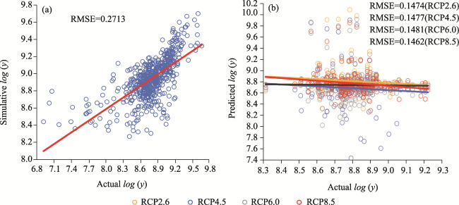
Figure 4 The ability of the statistical model to fit historical data and predict future data (a: historical data from 2000-2015; b: predicted data)

4 Results and analysis

4.1 Dynamic land use changes

The study area is projected to undergo notable changes in construction land, grassland, water areas, and unused land by 2050, but slight changes in cultivated land and woodland. These land use changes will exhibit evident spatial differences across the study area (Figures 5 and A3). The total area of cultivated land is expected to slightly increase from 43,321.70 km2 in 2010 to 43,556.00 km2 in 2050, with an inverted U-shaped trend. Specifically, the cultivated land will increase to 44,424.08 km2 in 2030 and then decrease by 867.61 km2 from 2030 to 2050. However, this trend will vary at the city level, with cultivated land in Changchun and Liaoyuan increasing by 485.68 km2 and 19.62 km2, respectively, from 2010 to 2050, while those in Tonghua, Jilin, and Siping decreasing by 252.12 km2, 11.33 km2, and 3.88 km2.
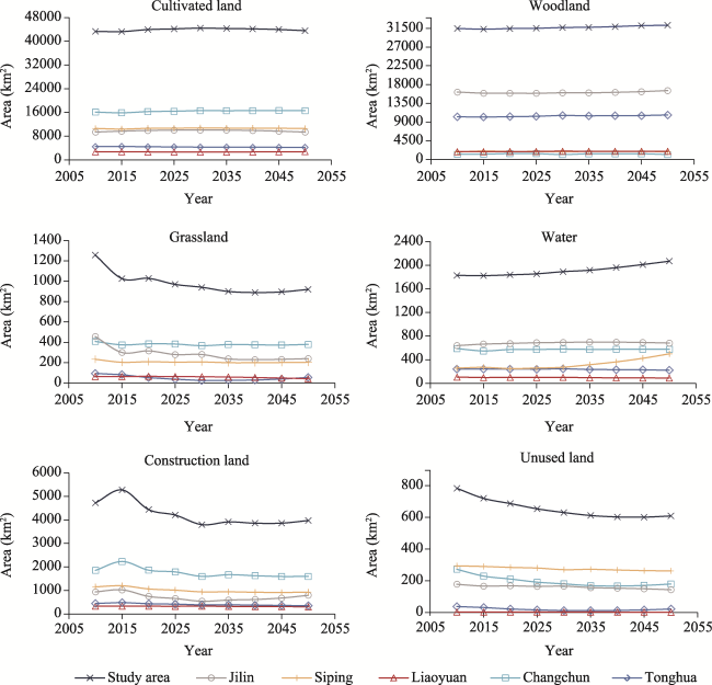
Figure 5 The changes in land use quantities in the central Jilin province of China from 2010 to 2050
The gain and loss of cultivated land will be 3,796.69 km2 and 3,561.53 km2, respectively (Figure 6f). The increase in cultivated land is mainly due to the conversion of woodland and construction land, which account for 43.09% and 40.03% of farmland gain, respectively. This is largely attributed to the consolidation of scattered rural settlements originating from rural population shrinkage. On the other hand, 63.71% of farmland loss is caused by farmland reforestation, indicating the Chinese emphasis on ecological protection (Shan et al., 2020). At the city level, Changchun shows the highest farmland gain, with an increase of 1,080.04 km2 (Figure 6a), and 59.45% of this gain comes from the consolidation of construction land. As a central city in Northeast China, the increase in cultivated land will help alleviate the pressure of the growing population on food production (Zhang et al., 2012). Conversely, Tonghua experiences the largest reduction of arable land (Figure 6e), with a net loss of 251.52 km2. Notably, 627.28 km2 of cultivated land in this city will be converted into forest land. Liaoyuan, Siping, and Jilin are likely to undergo slight changes in farmland, with a gain or loss of less than 20 km2 (Figures 6b, 6c, and 6d).
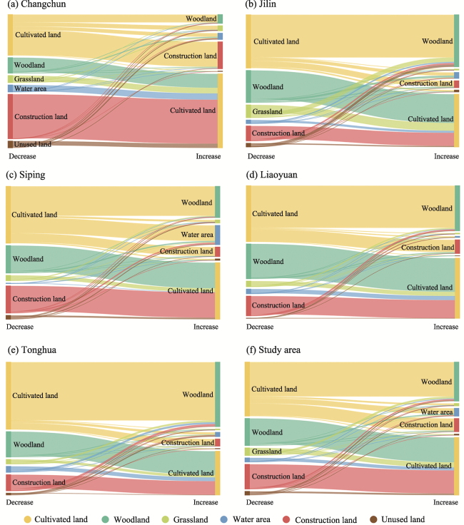
Figure 6 Land use conversions in the central Jilin province of China from 2010 to 2050 (ha)

4.2 Changes in maize yield per hectare in different scenarios

The maize yield per hectare is likely to exhibit a two-stage upward trend from 2011 to 2050 (Figure 7). From 2011 to 2030, it will moderately increase by 76.32%, 70.63%, 63.278%, and 49.66% under RCP2.6, RCP4.5, RCP6.0, and RCP8.5, respectively. From 2031 to 2050, however, the yield is expected to experience a corresponding sharp increase of 280.74%, 344.91%, 299.64%, and 233.352%, respectively.
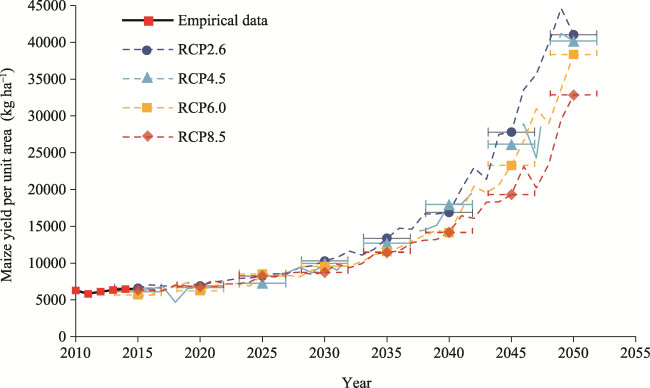
Figure 7 Changes in average maize yield in the central Jilin province of China under four scenarios from 2011 to 2050. Standard Errors of Mean (SEM) of RCP2.6, RCP4.5, RCP6.0, and RCP8.5 are 1575.51, 1401.41, 1252.26, and 975.38 kg ha-1, respectively.
Climate change may exert different effects on per unit maize yield over time (Figure A4). RCP2.6 is expected to have the maximum annual growth rate per unit yield, up to 34.73%, with a mean value of 14,175.00 kg ha-1. Conversely, RCP8.5 is likely to exhibit the minimum increase of the per unit yield by 11,324.47 kg ha-1 with an annual growth rate of 33.78%. A positive correlation can be observed between the per unit yield promotion and the radiative forcing levels caused by greenhouse gas emissions, and the gaps in the per unit yields between four RCP scenarios will also increase over time. We also found a strong correlation between temperature and the changing rate of the maize yield variance (Figure 8). In RCP2.6, RCP6.0, RCP8.5, R2 can reach up to 0.99 (p<0.0001), while that in RCP4.5 is only 47.21%. Temperature change primarily leads to yield variance.
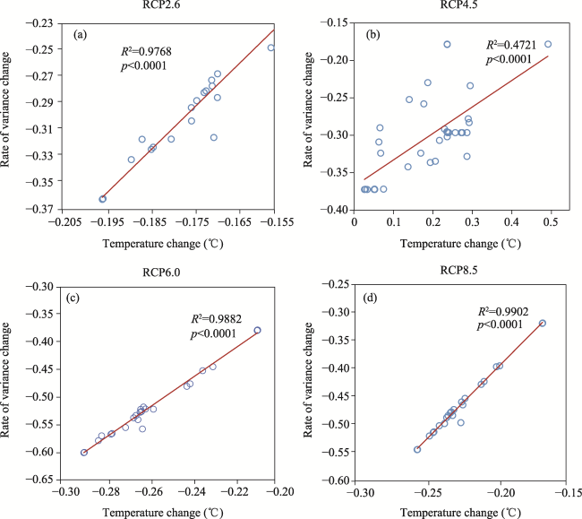
Figure 8 Correlation analysis between temperature and variance transformation rate under four scenarios
At the county level, the yield variations under the four RCPs range from 0.72 to 32.82 from 2011 to 2030, and from 0.82 to 32.87 in 2031-2050. However, the mean per unit yield gap between the four RCPs is projected to be much larger from 2031 to 2050. For example, the range of RCP2.6 in 2031-2050 can expand to ten times that of 2011-2030. Despite the different distribution of values, the mean yields still exhibit a positive correlation with the variances. The spatial distribution of relative change in the mean yield per hectare and its variance in these two periods are similar, with a significant increase in the northern and central regions and a slight change in the western region. Most counties experience a similar change rate of mean yield under the four RCPs, but the gaps under RCP2.6 and RCP6.5 are much larger (Figure 9a). From a distribution area perspective, RCP6.5 and RCP8.5 have a greater reduction of variance from 2011-2030 to 2031-2050 (Figure 9b).
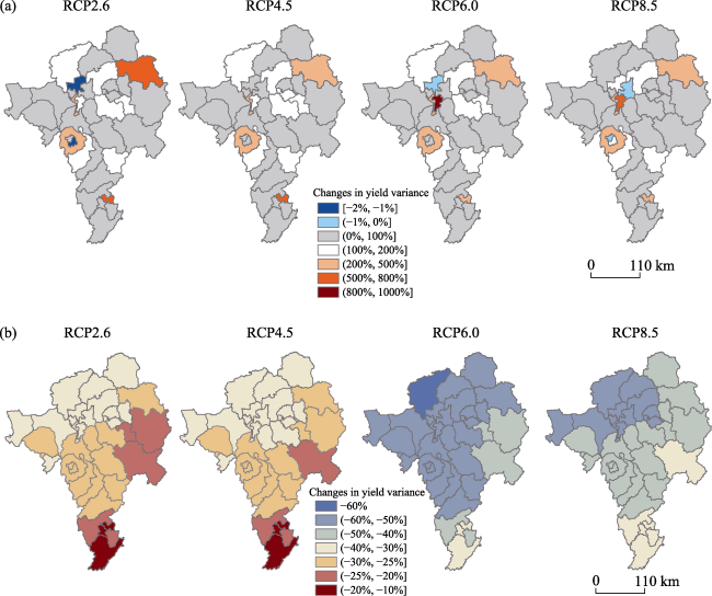
Figure 9 Changes in means (a) and variances (b) of the per unit maize yield in the central Jilin province of China during the periods of 2011-2030 (a) and 2031-2050 (b)

4.3 Changes in total maize yield

The total maize yield is expected to exhibit a significant increase from 2011 to 2050 under all four scenarios, with growth rates of 78.71% (RCP2.6), 79.40% (RCP4.5), 79.01% (RCP6.0) and 78.63% (RCP8.5). Over the first two decades, the total yield under RCP2.6, RCP4.5, RCP6.0, and RCP8.5 is projected to moderately increase by 38.61%, 35.61%, 30.03%, and 18.28%, respectively, followed by a sharp promotion to 124.92%, 149.01%, 148.19% and 161.00% in the latter twenty years. There will be significant differences in the total maize yields under the four RCP scenarios. Specifically, RCP2.6 has the maximum total yield of 24.02 megatons in 2030, but it will rank third in 2050. RCP4.5 is expected to rank second in 2030 with a maize yield of 23.50 megatons, but it will reach the highest value of 58.52 megatons in 2050. It is noteworthy that the total maize yield under RCP8.5 will remain the minimum in both 2030 and 2050 (Table 3).
Table 3 Total maize yields in 2030 and 2050 under four scenarios
Scenarios 2030 (megatons) Change rate 2011-2030 (%) 2050 (megatons) Change rate 2030-2050 (%)
RCP2.6 24.02 38.61 54.03 124.92
RCP4.5 23.50 35.61 58.52 149.01
RCP6.0 22.54 30.03 55.93 148.19
RCP8.5 20.50 18.28 53.50 161.00
The changes in total maize yields will be influenced by both climate change and the planting area (Figure 10). For example, some urban areas such as Changchun, Jilin, and Chaoyang have low total maize yields, despite having moderate or high per unit yield. Conversely, counties such as Nong’an and Gongzhuling with low per unit yields may have higher maize production due to their larger maize planting areas. Climate change will also alter the rankings of the counties with large maize planting areas, e.g., Liuhe, Lishu, Fengman, Dongliao, and Dongfeng County. Under PCR2.6, a slowdown in the growth rate of maize yield per hectare in these counties may lead to a decline in their total yield rankings. On the other hand, RCP8.5 may ensure that most counties have a high total production ranking due to its relatively high growth rate of per unit yield.
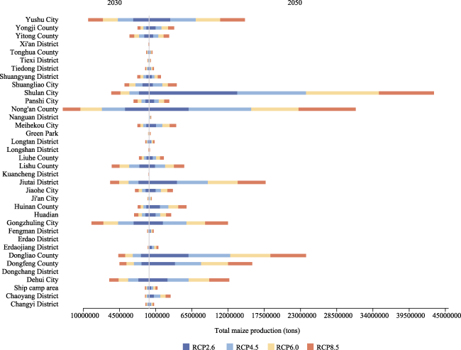
Figure 10 Total maize production at the county level in the central Jilin province of China under four scenarios
It is important to note that the total maize yield is equal to the yield per hectare multiplied by the planted area. An increase in unit maize yield could mitigate the impact of farmland loss on total regional maize production. For example, despite 67% of counties experiencing a decrease in cropland from 2030 to 2050 (Figure A5), total maize production in these counties is expected to increase due to the promotion of per hectare maize yield. In Tietong District, for instance, the reduction of 939.69 ha of cultivated land from 2030-2050 will reduce the total maize production by 2.87% under the four scenarios if the unit yield remains constant from 2030. However, under RCP4.5, RCP6.0, and RCP8.5, total maize production in Tietong will increase by 89,651.62 ton, 88,606.30 ton, and 152,395.44 ton, respectively, due to climate change and agricultural technology progress. Moreover, an increase in maize acreage in some regions can also mitigate the impact of low unit maize yield. In Dongfeng County, for instance, the unit maize yield will decrease by 60.35 kg ha-1 from 2030 to 2050 under the RCP8.5, and if the unit maize yield remains constant, the total maize yield will decrease by 0.99% in 2050. However, the increase in arable land area of 5932.93 ha is expected to cause an increase in total yield by 3.54%.

5 Discussion

5.1 Comprehensive impact on maize yield

We conducted our study in the black soil area of Jilin province to gain a spatially explicit understanding of the combined impact of climate change and land use change on the yield of rain-fed maize. Our findings align with previous research that identifies temperature as a crucial factor affecting spring maize yields in NEC, a cold temperate zone where increasing temperatures can extend the thermal growing season and reduce cold damage, thereby benefiting maize yields (Li et al., 2011; Li et al., 2016). Variations in temperature during the pre-flowering, flowering, and filling stages can lead to different degrees of maize yield reduction, with higher temperatures above 29°C causing significant reductions in maize yield (Lobell et al., 2011; Zhang et al., 2023). However, we found that the maximum temperature during the growing season in our study area did not exceed 30°C. Moreover, prior research suggests that an increase in minimum temperature during the growing season may benefit maize production in NEC (Wang et al., 2014), as warmer minimum temperatures can increase nighttime carbohydrate respiration losses, stimulating photosynthesis the following day (Peng et al., 2013) and reducing the incidence of frost in NEC (Chen et al., 2011). Our projections indicate that the average minimum temperatures during the growing season in our study area will increase by 0.36°C, 0.19°C, 0.46°C, and 0.41°C for the RCP2.6, RCP4.5, RCP6.0, and RCP8.5 scenarios, respectively, compared to the 2010-2030 period.
Our experiments showed a sharp increase in maize yield from 2031 to 2050. Previous studies have demonstrated that a 1°C increase in temperature can increase maize yields by more than 20% in parts of NEC (Wang et al., 2007) and that some areas could exceed 60 million kg ha-1 in 2050 (Pu et al., 2020). Figures A1 (a) and A4 (a) show that temperatures have been increasing across all four scenarios from 2010 to 2050. Under the RCP2.6, RCP4.5, RCP6.0, and RCP8.5, the average temperatures of maize growing season in the study area in 2030-2050 were 0.38°C, 0.20°C, 0.41°C, and 0.54°C higher than those in 2010-2030, respectively. Based on historical trends, we forecasted an increase in agricultural technology from 2010 to 2050, which resulted in a higher value for the machine variable in 2050-2030 than in 2010-2030. The combination of temperature increases and improved machinery will increase the unit yield of maize, leading us to predict that the unit maize yield will reach 40,000 kg ha-1 by 2050.
The results also revealed a clear contrast in total yield, potential increment, and spatial pattern between different scenarios. We found that balanced development is more conducive to maintaining a steady increase in total maize production. Specifically, we observed that the potential maize yield per hectare will significantly increase under the four climate change scenarios from 2011 to 2050, with RCP2.6, RCP4.5, RCP6.0, and RCP8.5 ranking in that order. However, RCP2.6 and RCP6.0 exhibited differences in maize yields among counties, while RCP4.5 demonstrated a balanced regional pattern of maize production (Figure 8a). The total maize yield in 2050 was projected to peak under RCP4.5, suggesting the combined positive effect of temperature, precipitation, and technological progress on maize growth. Moderate carbon emissions, population, and economic growth in this scenario can help coordinate the conflicts between farmland protection and vegetation conservation and increase overall maize production simultaneously (Zhang et al., 2010; Hou et al., 2021). It is worth noting that an increase in per hectare yield could mitigate the impact of farmland loss on maize yields. Despite a large amount of cultivated land being occupied by forest and grassland, the total maize yield under all scenarios still increased exponentially. The total yields of RCP2.6, RCP4.5, RCP6.0, and RCP8.5 will reach 54.03, 58.52, 55.93, and 53.50 megatons by 124.92%, 149.01%, 148.19%, and 161.00%, respectively, from 2030 to 2050.
The variance in temperature and precipitation during the growing season will affect yield variance (Urban et al., 2012). As precipitation variance increases, the variance of maize yields during the period of 2031-3050 will be higher than that in 2011-2030. Under the threat of maize yield reduction caused by variable or extreme climates (Feng et al., 2021; Malik et al., 2021), how to formulate adaptation and mitigation strategies will be a challenging long-term issue for land managers (Iglesias et al., 2015; Rutgersson et al., 2022).

5.2 Policy implications

Our study suggested several implications for agricultural land use and maize production. By considering the present and predicted near-future land use, economic and climate scenarios, we can solve many uncertainties in agricultural production. Specifically, we have developed differential maize yield protection systems for different maize production areas. In areas such as Jilin and Siping where there is severe depopulation, we recommend prohibiting the development of marginal land and seeking excellent new sources of arable land. For example, the government can encourage the reclamation of abandoned rural areas into agricultural land by integrating scattered rural settlements. In Tonghua, which is consistently located in a low-value area for maize production, we suggest optimizing its cropping structure and initiatives to ensure the sustainable use of cultivated land, such as a fallow system in conjunction with local land capacity and water resources, and increased subsidies for insurance premiums with high planting risks (such as producer subsidies for planting alternative crops such as rice and wheat). In Changchun, areas such as Nongan, Gongzhuling, and Yushu counties have wide cropland due to topographic features and high maize yields resulting in consistently high maize production. The government should strengthen the management and protection of cultivated land in the region to avoid degradation. Meanwhile, policy-makers should consider the strategic synergy between economic development policies and cultivated land use, including the adjustment of the compensation balance policy for cultivated land expropriation.
Moreover, agricultural technology development can balance land use change, climate change and maize production due to its positive impact on per unit yield (Rojas-Downing et al., 2017). Previous studies suggested that the diversification of maize varieties could improve maize resistance to external disturbances caused by extreme weather events and human activities (Altieri et al., 2017). Maize breeding and biotechnology also have enormous biological potential to increase grain yield (Foulkes et al., 2011). Researchers have proven that organic matter enhances underground biodiversity, thereby creating suitable conditions for plant roots (Diaz-Zorita et al., 1999; Morugan-Coronado et al., 2022). In addition, proper agricultural management, such as organic agriculture, residue management and crop rotation, can also improve soil quality (Morugan-Coronado et al., 2022). Moreover, regular training and technical guidance for farmers can improve their risk awareness and ability to address risk (Olesen et al., 2011). In summary, we recommend investing in maize variety and planting technology development to promote the per unit yield of maize. An accurate prediction of climate change and the rational planning of planting scale and planting pattern can advance the reasonability of agricultural management strategies.

5.3 Strengths and limitations

The research framework developed in this study integrates the FLUS and statistical yield model to provide a comprehensive understanding of the joint impact of climate change and land use change on maize yield. This flexible framework can serve as a useful decision-making tool for land planning and maize management in diverse scenarios. The study findings reveal that climate change is likely to have a positive effect on maize yields in the study area, which aligns with previous simulation studies (Liang et al., 2019; Pu et al., 2020). As the study area is situated in the cold temperate zone, global warming could mitigate cold damage and prolong the growing season, resulting in improved maize yields. It is encouraging to note that advancements in agricultural technology and management practices may further enhance planting efficiency in the future. Notably, this study excluded the impact of human irrigation by selecting a rain-fed region for analysis.
Future research can focus on two issues. One major issue is the potential uncertainty associated with future climate change, which can affect the accuracy of simulation results. Different general circulation models (GCMs) may produce varying climate projections for the same region, resulting in discrepancies in simulation outcomes (Manatsa et al., 2011). To address this issue, the BCC_CSM1.1 m model was employed in this study to reduce the potential errors in prediction. Although the BCC has been applied to multiple studies on grain production in NEC (Pu et al., 2020; Xie et al., 2020), there is still room for improvement. Another issue is that previous research has suggested that incorporating remote sensing data into statistical models can improve forecasting accuracy, particularly for large-scale regions (Laudien et al., 2020).

6 Conclusions

This study proposed an integrated framework for maize yield prediction by combining the SD and FLUS models with a statistical model. The proposed framework is flexible and applicable to regional studies and can simulate future yield changes under the four RCP scenarios. The simulations provide guidance for agricultural management decision-making.
The study concluded that an increase in per-unit yield could mitigate the negative impact of farmland loss on total maize yield. Despite the expected decrease in cultivated land from 2030 to 2050, the total maize yields under RCP2.6, RCP4.5, RCP6.0, and RCP8.5 are projected to increase by 124.92%, 149.01%, 148.19%, and 161.00%, respectively. However, the disparities in total maize yields will vary across the region, especially under RCP2.6, while RCP4.5 is expected to be more balanced and stable, benefitting regional sustainable development. To address the challenges posed by variable or extreme climates and the widening yield gap between counties, differentiated policies for agricultural production and farmland protection need to be implemented. These measures may include strengthened cultivated land protection and crop management in low-yield areas and the adoption of adaptation and mitigation measures.

Text A1

The improvement in agricultural mechanization (machine, machine2) and county-fixed effects (county) explain 40.3% of the county-level yield variance, which reflects the mean and the rapid improvement pace of crop have presented uneven spatial distribution since 2000. T, P, and their square terms explain 3.3% of the county-level production variance. Sunshine hours (SH) has an insignificant coefficient of determination, and is excluded in the final model (Equation A1). Table A1 shows the model coefficient and significance test.
$\begin{align} & \log \left( yeild \right)=0.000128*machin{{e}^{2}}-0.0055*machine+1.598*T-0.043*{{T}^{2}}+ \\ & \text{ }0.006394*P-0.0000262*{{P}^{2}}-6.234 \end{align}$
Considering the error value, the model can be written as:
$\log \left( {{y}_{county\text{,}year}} \right)=\log \left( {{{\hat{y}}}_{county\text{,}year}} \right)+\log \left( {{\text{ }\!\!\varepsilon\!\!\text{ }}_{county\text{,}year}} \right)$
The hat symbol (^) indicates the estimated value of yield production. Assume that the error is independent of the estimated value $\log \left( \text{ }\!\!\varepsilon\!\!\text{ } \right)$. All terms in the above equation are logarithmic. We first take the exponents on both sides of Equation A2 to calculate the yield per hectare.
$y={{e}^{\log \left( {\hat{y}} \right)}}{{e}^{\log \left( \text{ }\!\!\varepsilon\!\!\text{ } \right)}}$
It is crucial to consider the yield error when we compare the yield variance between 2011-2030 and 2031-2050. We can calculate the variance of the final production, substituting the variance values of the residuals at all levels (Attached Table A2):
$\begin{align} & Var\left( y \right)={{\left( E\left[ \log \left( {\hat{y}} \right) \right] \right)}^{2}}\times Var\left( \log \left( \text{ }\!\!\varepsilon\!\!\text{ } \right) \right)+{{\left( E\left[ \log \left( \text{ }\!\!\varepsilon\!\!\text{ } \right) \right] \right)}^{2}}\times Var\left( \log \left( {\hat{y}} \right) \right)+ \\ & \text{ }Var\left( \log \left( {\hat{y}} \right) \right)\times Var\left( \log \left( \text{ }\!\!\varepsilon\!\!\text{ } \right) \right) \end{align}$
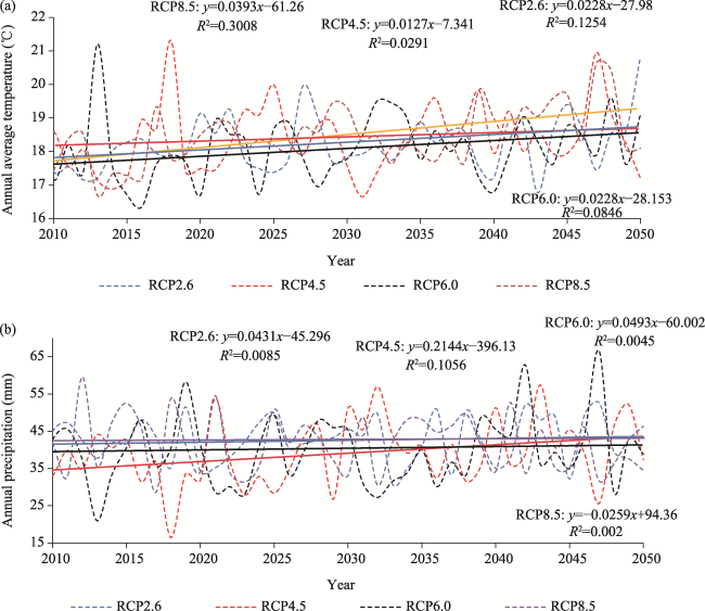
Figure A1 Annual average temperature from May to September under RCPs (a); annual precipitation in the central Jilin province of China from May to September under RCPs (b)
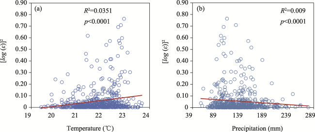
Figure A2 Least-squares regression of the square of the production residuals and the annual average temperature (a) and annual precipitation (b) during the training period
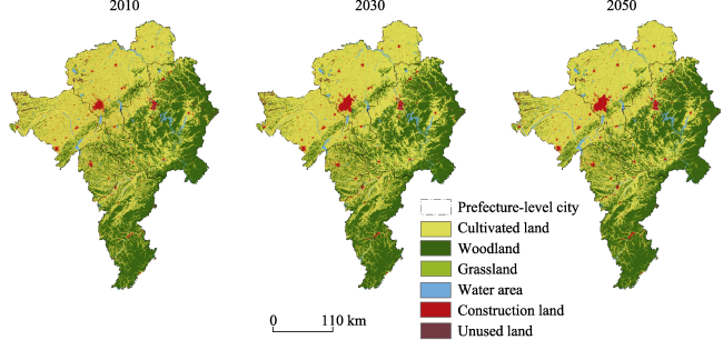
Figure A3 Land use maps of the central Jilin province of China in 2010, 2030 and 2050
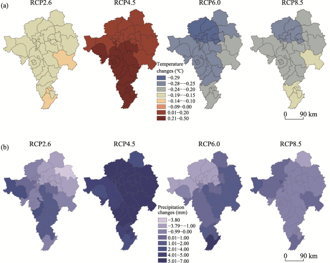
Figure A4 Temperature variation by county (a), and precipitation variation by county (b) in the central Jilin province of China from 2011-2030 to 2031-2050 under four scenarios
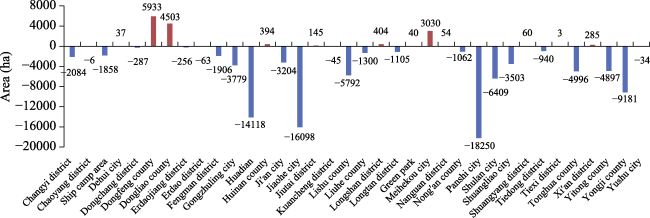
Figure A5 Changes in cultivated land areas at county level in the central Jilin province of China from 2030 to 2050
Table A1 Regression coefficients
Model Unstandardized coefficient t Sig.
B Standard error
(constant) -6.226 7.759 -0.802 0.423
T 1.598 0.788 2.029 0.043
T2 -0.043 0.020 -2.163 0.031
P 0.006 0.003 2.254 0.025
P2 -2.622E-05 0.000 -2.146 0.032
machine -0.006 0.001 -4.633 0.000
machine2 1.284E-04 0.000 3.153 0.002
SH 2.750E-04 8.02 E-04 0.342 0.732
Area=Dongfeng County 0.243 0.104 2.329 0.020
Area=Dongchang District 0.265 0.135 1.971 0.049
Area=Dongliao County 0.251 0.105 2.392 0.017
Area = Fengman District 0.095 0.115 0.821 0.412
Area=Jiutai City 0.035 0.104 0.342 0.733
Area = Erdao District -0.409 0.102 -4.025 0.000
Area = Erdaojiang District 0.148 0.134 1.105 0.269
Area=Yitong County 0.267 0.102 2.623 0.009
Area=Gongzhuling City 0.652 0.105 6.212 0.000
Area=Nong'an County 0.431 0.105 4.085 0.000
Area = Nanguan District -0.019 0.109 -0.173 0.863
Area=Shuangyang District 0.316 0.108 2.920 0.004
Area = Kuancheng District -0.400 0.102 -3.920 0.000
Area=Dehui City 0.298 0.106 2.813 0.005
Area=Changyi District 0.092 0.103 0.888 0.375
Area=Chaoyang District -0.106 0.113 -0.942 0.346
Area = Liuhe County 0.255 0.112 2.263 0.024
Area = Huadian City -0.020 0.121 -0.167 0.867
Area=Meihekou City 0.087 0.104 0.834 0.405
(constant) -6.226 7.759 -0.802 0.423
Area = Lishu County 0.724 0.105 6.916 0.000
Area = Elm City 0.313 0.104 3.019 0.003
Area=Yongji County 0.028 0.103 0.268 0.788
Area=Panshi City 0.106 0.103 1.024 0.306
Area = Green Park 0.055 0.119 0.461 0.645
Area = Shulan City 0.200 0.111 1.810 0.071
Area = Ship Camp Area 0.063 0.105 0.599 0.549
Area = Jiaohe City 0.102 0.116 0.877 0.381
Area = Xi'an District -0.042 0.103 -0.412 0.680
Area=Huinan County 0.351 0.112 3.130 0.002
Area=Tonghua County -0.051 0.110 -0.460 0.646
Area=Tiedong District 0.236 0.107 2.200 0.028
Area = Tiexi District 0.449 0.185 2.427 0.016
Area = Ji'an City -0.098 0.109 -0.894 0.372
Area = Longshan District -0.055 0.102 -0.538 0.591
Area=Longtan District 0.091 0.105 0.868 0.386

Note: B and Beta are regression coefficients; Sig. is the P-value, which represents the significance in the hypothesis test.

Table A2 Variance of county residual error
Region $Var\left( \log \left( \epsilon \right) \right)$ Region $Var\left( \log \left( \epsilon \right) \right)$
Changyi District 0.025572075 Liuhe County 0.044541441
Chaoyang District 0.195618882 Yongsan District 0.088251022
Ship Camp Area 0.014275893 Longtan District 0.019158748
Dehui 0.033632781 Green Park 0.249584034
Dongchang District 0.014318566 Meihekou 0.009294256
Dongfeng County 0.026302486 Nanguan District 0.14462959
Dongliao County 0.049171297 Nong'an County 0.011689685
Erdaojiang District 0.031237137 rock city 0.01400162
Erdao District 0.431996676 Shulan 0.01074008
plump area 0.048536536 Shuangliao 0.038542727
Gongzhuling 0.010237088 Shuangyang District 0.072074432
Huadian 0.026221195 Tiedong District 0.039590128
Huinan County 0.070030835 Tiexi District 0.079287917
Ji'an 0.023745877 Tonghua County 0.011766734
Jiaohe 0.046481507 Xi'an District 0.344605244
Jiutai District 0.0508169 Yitong County 0.071153589
Kuancheng District 0.28749462 Yongji County 0.043845527
Lishu County 0.030609236 Elm City 0.012829379
Table A3 The relation functions used in the SD model
Dependent variable Independent variable
Changchun Jilin Siping Liaoyuan Tonghua
Population change Population change rate ×Total population
Agricultural population Agricultural population ratio ×Total population
Construction land change Population change × Construction land per capita
Construction land per capita 0.02808×(Time-2015) + 2.36822
Total grain production 196696×
(Time-2015) + 7.02149e+06
38568.5×
(Time-2015)+ 3.61855e+06
223246×
(Time-2015)+
5.19641e+06
17327.5×
(Time-2015) + 1.213e+06
17500.5×
(Time-2015)+ 1.62026e+06
Technology expenditure ratio 6.5×(Time-2015)+ 0.009628 6.38×(Time-2015)+ 0.005389 76.109×
(Time-2015)- 1977.53
27.5×
(Time-2015) + 1.23277e+06
1.089×(Time-2015)+ 0.008784
Forestry output value 1977.86×
(Time-2015) + 8967.88
6855.19×
(Time-2015) + 32268.6
765.905×
(Time-2015)+
12584
2158.23×
(Time-2015) - 2693.16
11005.8×
(Time-2015) - 22992.2
Technology expenditure 7437.71×
(Time-2015) -
17716.6
4166.49×
(Time-2015) - 10044.6
761.109×
(Time-2015) - 1977.53
804.273×
(Time-2015)- 2886.62
5366.08×
(Time-2015) - 20759.7
Pastoral output value 144195×
(Time-2015)+ 1.15857e+06
138068×
(Time-2015)+ 249054
213037×
(Time-2015)+ 556231
38851.8×
(Time-2015)+ 118363
31078.9×
(Time-2015)+ 216560
Fishery output value 4235.14×
(Time-2015) -
1124.15
6211.77×
(Time-2015) + 38328.4
1548.15×
(Time-2015)- 5607.55
611.483×
(Time-2015) - 1412.13
3972.97×
(Time-2015)+ 2054.63
Proportion of expenditure on agriculture 0.0027×
(Time-2015) +
0.0395
0.0027×
(Time-2015)+ 0.0395
-0.001092×
(Time-2015)+ 0.129638
0.000930×
(Time-2015)+ 0.0866
-0.001715×
(Time-2015)+ 0.1312
Total power of agricultural
machinery
21.428 × (Time-2015)+
205.236
25.8394×
(Time-2015)+ 63.2892
18.9625×
(Time-2015)+ 81.9124
10.4513×
(Time-2015) + 2.82133
6.58964×
(Time-2015)+ 84.9691
Cultivated land change -109.732+0.0976×
Total power of agricultural machinery+ 0.195929×
Agricultural population- 1.25146e-06× Total grain production
-108.152+0.0896×
Total power of agricultural machinery+ 0.172859× Agricultural population-1.20816e-06×
Total grain production
-107.362+0.0976×Total power of agricultural machinery+ 0.29653×Agricultural population+ 1.25146e-06× Total grain production -45+0.0976×Total power of agricultural machinery+ 0.2× Agricultural population+ 1.25146e-06×Total grain production -52.732+0.0976× Total power of agricultural machinery+ 0.195929× Agricultural population+ 1.25146e- 06×Total grain production
Water area change 0.4719-2.48582e-05
×Fishery output
value-
9.75115×
Proportion of
expenditure on agriculture-
0.0114061×
Unused land
0.3287+2e-05× Fishery output value- 9.7× Proportion of expenditure on agriculture+ 0.014025×Unused land 0.2693+2e-05× Fishery output value- 9.67103× Proportion of expenditure on agriculture+ 0.0100651×Unused land 0.4+2e-05×Fishery output value- 9.35115×Proportion of expenditure on agriculture+ 0.01×Unused land 0.4178+2e-05× Fishery output value- 9.5115× Proportion of expenditure on agriculture+ 0.024551×Unused land
Grassland change 71.451-0.041978× Woodland -0.0281294×Total power of agricultural machinery+ 1.83056e-07×Pastoral output value-45.069× Technology expenditure ratio 69.451-0.004× Woodland + 0.0311575× Total power of agricultural machinery+ 1.83056e-07× Pastoral output value- 38.405× Technology expenditure ratio 70.895-0.04× Woodland +0.03× Total power of agricultural machinery+ 2.0056e-07× Pastoral output value+41.036× Technology expenditure ratio 64.589-0.035× Woodland + 0.0281294×Total power of agricultural machinery- 1.83056e-07× Pastoral output value-40.853× Technology expenditure ratio 75.186-0.0066× Woodland -0.028× Total power of agricultural machinery-1.8e-07× Pastoral output value+10.853× Technology expenditure ratio
Woodland change 52.0559-0.096× Grassland+ 0.000108421×
Forestry output value+ 0.0001×Technology expenditure
46.0559-0.096× Grassland+ 0.000108421× Forestry output value+ 0.0001× Technology
expenditure
32.0559-0.097× Grassland- 0.000108421× Forestry output value+0.0001× Technology
expenditure
28-0.1×Grassland- 0.00011×Forestry output value +0.001× Technology expenditure 40.0559-0.0966744×Grassland- 0.000108421× Forestry output value- 0.0001× Technology expenditure
Unused land 20528-Cultivated land-Grassland- Woodland -Water area- Construction land 27782.1-Cultivated land-Grassland- Woodland -Water area- Construction land 14355.2-Cultivated land-Grassland- Woodland -Water area- Construction land 5144.74-Cultivated land-Grassland- Woodland -Water area- Construction land 15568.6-Cultivated land-Grassland- Woodland -Water area- Construction land
[1]
Abate M C, Kuang Y-P, 2021. The impact of the supply of farmland, level of agricultural mechanisation, and supply of rural labour on grain yields in China. Studies in Agricultural Economics, 123(1): 33-42.

[2]
Akhtar M K, Wibe J, Simonovic S P et al., 2013. Integrated assessment model of society-biosphere-climate-economy-energy system. Environmental Modelling & Software, 49: 1-21.

[3]
Akpoti K, Kabo-bah A T, Zwart S J, 2019. Agricultural land suitability analysis: State-of-the-art and outlooks for integration of climate change analysis. Agricultural Systems, 173: 172-208.

DOI

[4]
Altieri M A, Nicholls C I, 2017. The adaptation and mitigation potential of traditional agriculture in a changing climate. Climatic Change, 140(1): 33-45.

DOI

[5]
Archontoulis S V, Miguez F E, Moore K J, 2014. Evaluating APSIM maize, soil water, soil nitrogen, manure, and soil temperature modules in the Midwestern United States. Agronomy Journal, 106(3): 1025-1040.

DOI

[6]
Asseng S, Ewert F, Rosenzweig C et al., 2013. Uncertainty in simulating wheat yields under climate change. Nature Climate Change, 3(9): 827-832.

DOI

[7]
Banakara K B, Pandya H R, Garde Y A, 2019. Pre-harvest forecast of kharif rice yield using PCA and MLR technique in Naysari district of Gujarat. Journal of Agrometeorology, 21(3): 336-343.

DOI

[8]
Basse R M, Omrani H, Charif O et al., 2014. Land use changes modelling using advanced methods - Cellular automata and artificial neural networks: The spatial and explicit representation of land cover dynamics at the cross-border region scale. Applied Geography, 53: 160-171.

DOI

[9]
Basso B, Liu L, 2019. Seasonal crop yield forecast: Methods, applications, and accuracies. Advances in Agronomy, 154: 201-255.

DOI

[10]
Basso B, Liu L, Ritchie J T, 2016. A comprehensive review of the CERES-wheat, -maize and -rice models’ performances. Advances in Agronomy, 136: 27-132.

[11]
Camberlin P, Diop M, 1999. Inter-relationships between groundnut yield in Senegal, interannual rainfall variability and sea-surface temperatures. Theoretical and Applied Climatology, 63(3/4): 163-181.

DOI

[12]
Chen C Q, Lei C X, Deng A X et al., 2011. Will higher minimum temperatures increase corn production in Northeast China? An analysis of historical data over 1965-2008. Agricultural and Forest Meteorology, 151(12): 1580-1588.

DOI

[13]
Diaz-Zorita M, Buschiazzo D E, Peinemann N, 1999. Soil organic matter and wheat productivity in the semiarid argentine pampas. Agronomy Journal, 91(2): 276-279.

DOI

[14]
Feng S, Hao Z, Zhang X et al., 2021. Changes in climate-crop yield relationships affect risks of crop yield reduction. Agricultural and Forest Meteorology, 304: 108401.

[15]
Foulkes M J, Slafer G A, Davies W J et al., 2011. Raising yield potential of wheat (III): Optimizing partitioning to grain while maintaining lodging resistance. Journal of Experimental Botany, 62(2): 469-486.

DOI PMID

[16]
Gao J, Liu L, Guo L et al., 2023. The effects of climate change and phenological variation on agricultural production and its risk pattern in the black soil area of northeast China. Journal of Geographical Sciences, 33(1): 37-58.

DOI

[17]
Gao J Q, Yang X G, Zheng B Y et al., 2020. Does precipitation keep pace with temperature in the marginal double-cropping area of northern China? European Journal of Agronomy, 120: 126126.

DOI

[18]
Giri A K, Bhan M, Agrawal K K, 2017. Districtwise wheat and rice yield predictions using meteorological variables in eastern Madhya Pradesh. Journal of Agrometeorology, 19(4): 366-368.

DOI

[19]
Grassini P, Yang H S, Cassman K G, 2009. Limits to maize productivity in Western Corn-Belt: A simulation analysis for fully irrigated and rainfed conditions. Agricultural and Forest Meteorology, 149(8): 1254-1265.

DOI

[20]
He Y, Liang H, Hu K L et al., 2018. Modeling nitrogen leaching in a spring maize system under changing climate and genotype scenarios in arid Inner Mongolia, China. Agricultural Water Management, 210: 316-323.

DOI

[21]
Hengl T, de Jesus J M, Heuvelink G B M et al., 2017. SoilGrids250m: Global gridded soil information based on machine learning. Plos One, 12(2): e0169748.

DOI

[22]
Hou R, Li H, 2021. Spatial-temporal change and coupling coordination characteristics of land use functions in Wuhan City: Based on the comparison before and after the resource-economical and environment-friendly society experimental zone establishment. China Land Science, 35(1): 69-78. (in Chinese)

[23]
Huang J, Tang Z, Liu D et al., 2020. Ecological response to urban development in a changing socio-economic and climate context: Policy implications for balancing regional development and habitat conservation. Land Use Policy, 97: 104772.

DOI

[24]
Huang J Y, Hartemink A E, Kucharik C J, 2021. Soil-dependent responses of US crop yields to climate variability and depth to groundwater. Agricultural Systems, 190: 103085.

[25]
Iglesias A, Garrote L, 2015. Adaptation strategies for agricultural water management under climate change in Europe. Agricultural Water Management, 155: 113-124.

DOI

[26]
Jiang R, He W T, He L et al., 2021. Modelling adaptation strategies to reduce adverse impacts of climate change on maize cropping system in Northeast China. Scientific Reports, 11(1): 810.

DOI PMID

[27]
Kang Y H, Ozdogan M, Zhu X J et al., 2020. Comparative assessment of environmental variables and machine learning algorithms for maize yield prediction in the US Midwest. Environmental Research Letters, 15(6): 064005.

[28]
Knutti R, 2014. IPCC Working Group I AR5 snapshot: The rcp26 experiment. Retrieved from: https://doi.org/10.1594/WDCC/ETHr2.

[29]
Kolotii A, Kussul N, Shelestov A et al., 2015. Comparison of biophysical and satellite predictors for wheat yield forecasting in Ukraine. 36th International Symposium on Remote Sensing of Environment, 47(w3): 39-44.

[30]
Kowalik W, Dabrowska-Zielinska K, Meroni M et al., 2014. Yield estimation using SPOT-VEGETATION products: A case study of wheat in European countries. International Journal of Applied Earth Observation and Geoinformation, 32: 228-239.

DOI

[31]
Kriegler E, Edmonds J, Hallegatte S et al., 2014. A new scenario framework for climate change research: The concept of shared climate policy assumptions. Climatic Change, 122(3): 401-414.

DOI

[32]
Laudien R, Schauberger B, Makowski D et al., 2020. Robustly forecasting maize yields in Tanzania based on climatic predictors. Scientific Reports, 10(1): 19650.

DOI PMID

[33]
Leng G, Hall J W, 2020. Predicting spatial and temporal variability in crop yields: An inter-comparison of machine learning, regression and process-based models. Environmental Research Letters, 15(4): 044027.

DOI

[34]
Li E, Zhao J, Pullens J W M et al., 2022. The compound effects of drought and high temperature stresses will be the main constraints on maize yield in Northeast China. Science of the Total Environment, 812: 152461.

DOI

[35]
Li X, Chen G Z, Liu X P et al., 2017. A new global land-use and land-cover change product at a 1-km resolution for 2010 to 2100 based on human-environment interactions. Annals of the American Association of Geographers, 107(5): 1040-1059.

DOI

[36]
Li Y, Conway D, Xiong W et al., 2011. Effects of climate variability and change on Chinese agriculture: A review. Climate Research, 50(1): 83-102.

DOI

[37]
Li Y, Hu Z, Wang X et al., 2020. Characterization of a polysaccharide with antioxidant and anti-cervical cancer potentials from the corn silk cultivated in Jilin province. International Journal of Biological Macromolecules, 155: 1105-1113.

DOI PMID

[38]
Li Z, Tan J, Tang P et al., 2016. Spatial distribution of maize in response to climate change in northeast China during 1980-2010. Journal of Geographical Sciences, 26(1): 3-14.

DOI

[39]
Liang S, Zhang X B, Sun N et al., 2019. Modeling crop yield and nitrogen use efficiency in wheat and maize production systems under future climate change. Nutrient Cycling in Agroecosystems, 115(1): 117-136.

DOI

[40]
Lin Y M, Wu W X, Ge Q S, 2015. CERES-Maize model-based simulation of climate change impacts on maize yields and potential adaptive measures in Heilongjiang province, China. Journal of the Science of Food and Agriculture, 95(14): 2838-2849.

DOI PMID

[41]
Liu X, Liang X, Li X et al., 2017. A future land use simulation model (FLUS) for simulating multiple land use scenarios by coupling human and natural effects. Landscape and Urban Planning, 168: 94-116.

DOI

[42]
Liu Y, Ren H L, Klingaman N P et al., 2021. Improving long-lead seasonal forecasts of precipitation over Southern China based on statistical downscaling using BCC_CSM1.1m. Dynamics of Atmospheres and Oceans, 94: 101222.

DOI

[43]
Lobell D B, Burke M B, 2010. On the use of statistical models to predict crop yield responses to climate change. Agricultural and Forest Meteorology, 150(11): 1443-1452.

DOI

[44]
Lobell D B, Schlenker W, Costa-Roberts J, 2011. Climate trends and global crop production since 1980. Science, 333(6042): 616-620.

DOI PMID

[45]
Loboguerrero A M, Campbell B M, Cooper P J M et al., 2019. Food and earth systems: Priorities for climate change adaptation and mitigation for agriculture and food systems. Sustainability, 11(5): 1372.

DOI

[46]
Malik M A, Wani A H, Mir S H et al., 2021. Elucidating the role of silicon in drought stress tolerance in plants. Plant Physiology and Biochemistry, 165: 187-195.

DOI PMID

[47]
Manatsa D, Nyakudya I W, Mukwada G et al., 2011. Maize yield forecasting for Zimbabwe farming sectors using satellite rainfall estimates. Natural Hazards, 59(1): 447-463.

DOI

[48]
Morugan-Coronado A, Perez-Rodriguez P, Insolia E et al., 2022. The impact of crop diversification, tillage and fertilization type on soil total microbial, fungal and bacterial abundance: A worldwide meta-analysis of agricultural sites. Agriculture Ecosystems & Environment, 329: 107867.

DOI

[49]
Murchie E H, Niyogi K K, 2011. Manipulation of photoprotection to improve plant photosynthesis. Plant Physiology, 155(1): 86-92.

DOI PMID

[50]
Mustafa A, Heppenstall A, Omrani H et al., 2018. Modelling built-up expansion and densification with multinomial logistic regression, cellular automata and genetic algorithm. Computers Environment and Urban Systems, 67: 147-156.

DOI

[51]
Ning J, Liu J, Kuang W et al., 2018. Spatiotemporal patterns and characteristics of land-use change in China during 2010-2015. Journal of Geographical Sciences, 28(5): 547-562.

DOI

[52]
O'Neill B C, Kriegler E, Riahi K et al., 2014. A new scenario framework for climate change research: The concept of shared socioeconomic pathways. Climatic Change, 122(3): 387-400.

DOI

[53]
Olesen J E, Trnka M, Kersebaum K C et al., 2011. Impacts and adaptation of European crop production systems to climate change. European Journal of Agronomy, 34(2): 96-112.

DOI

[54]
Pan Z, He J, Liu D et al., 2020. Predicting the joint effects of future climate and land use change on ecosystem health in the Middle Reaches of the Yangtze River Economic Belt, China. Applied Geography, 124: 102293.

DOI

[55]
Peng S S, Piao S L, Ciais P et al., 2013. Asymmetric effects of daytime and night-time warming on Northern Hemisphere vegetation. Nature, 501(7465): 88.

DOI

[56]
Peralta N R, Assefa Y, Du J et al., 2016. Mid-season high-resolution satellite imagery for forecasting site-specific corn yield. Remote Sensing, 8(10): 848.

DOI

[57]
Pontius R G, Boersma W, Castella J C et al., 2008. Comparing the input, output, and validation maps for several models of land change. Annals of Regional Science, 42(1): 11-37.

DOI

[58]
Poornima S, Pushpalatha M, 2019. Prediction of rainfall using intensified LSTM based recurrent neural network with weighted linear units. Atmosphere, 10(11): 668.

DOI

[59]
Pu L M, Zhang S W, Yang J H et al., 2020. Assessing the impact of climate changes on the potential yields of maize and paddy rice in Northeast China by 2050. Theoretical and Applied Climatology, 140(1/2): 167-182.

DOI

[60]
Rao A, Chandran M A S, Bal S K et al., 2022. Evaluating area-specific adaptation strategies for rainfed maize under future climates of India. Science of the Total Environment, 836: 155511.

DOI

[61]
Rojas O, 2007. Operational maize yield model development and validation based on remote sensing and agro-meteorological data in Kenya. International Journal of Remote Sensing, 28(17): 3775-3793.

DOI

[62]
Rojas-Downing M M, Nejadhashemi A P, Harrigan T et al., 2017. Climate change and livestock: Impacts, adaptation, and mitigation. Climate Risk Management, 16: 145-163.

DOI

[63]
Rotz S, Gravely E, Mosby I et al., 2019. Automated pastures and the digital divide: How agricultural technologies are shaping labour and rural communities. Journal of Rural Studies, 68: 112-122.

DOI

[64]
Rutgersson A, Kjellstrom E, Haapala J et al., 2022. Natural hazards and extreme events in the Baltic Sea region. Earth System Dynamics, 13(1): 251-301.

DOI

[65]
Sakamoto T, 2020. Incorporating environmental variables into a MODIS-based crop yield estimation method for United States corn and soybeans through the use of a random forest regression algorithm. Isprs Journal of Photogrammetry and Remote Sensing, 160: 208-228.

DOI

[66]
Shan Y, Huang Q, Guan D et al., 2020. China CO2 emission accounts 2016-2017. Scientific Data, 7(1): 54.

DOI

[67]
Sharma L K, Bali S K, Dwyer J D et al., 2017. A case study of improving yield prediction and sulfur deficiency detection using optical sensors and relationship of historical potato yield with weather data in maine. Sensors, 17(5): 1095.

DOI

[68]
Shi W, Tao F, Zhang Z, 2013. A review on statistical models for identifying climate contributions to crop yields. Journal of Geographical Sciences, 23(3): 567-576.

DOI

[69]
Tripathy R, Chaudhari K N, Mukherjee J et al., 2013. Forecasting wheat yield in Punjab state of India by combining crop simulation model WOFOST and remotely sensed inputs. Remote Sensing Letters, 4(1): 19-28.

DOI

[70]
Urban D, Roberts M J, Schlenker W et al., 2012. Projected temperature changes indicate significant increase in interannual variability of U.S. maize yields. Climatic Change, 112(2): 525-533.

DOI

[71]
van Vuuren D P, Carter T R, 2014. Climate and socio-economic scenarios for climate change research and assessment: Reconciling the new with the old. Climatic Change, 122(3): 415-429.

DOI

[72]
Vancutsem C, Marinho E, Kayitakire F et al., 2013. Harmonizing and combining existing land cover/land use datasets for cropland area monitoring at the African continental scale. Remote Sensing, 5(1): 19-41.

DOI

[73]
Vermeulen S J, Aggarwal P K, Ainslie A et al., 2012. Options for support to agriculture and food security under climate change. Environmental Science & Policy, 15(1): 136-144.

[74]
Wang X H, Peng L Q, Zhang X P et al., 2014. Divergence of climate impacts on maize yield in Northeast China. Agriculture Ecosystems & Environment, 196: 51-58.

DOI

[75]
Wang Y P, Chang K W, Chen R K et al., 2010. Large-area rice yield forecasting using satellite imageries. International Journal of Applied Earth Observation and Geoinformation, 12(1): 27-35.

DOI

[76]
Wang Z M, Song K S, Li X Y et al., 2007. Effects of climate change on yield of maize in maize zone of Songnen Plain in the past 40 years. Arid Zone Resources and Environment, (9): 112-117. (in Chinese)

[77]
Wu T W, Yu R C, Zhang F et al., 2010. The Beijing Climate Center atmospheric general circulation model: Description and its performance for the present-day climate. Climate Dynamics, 34(1): 123-147.

DOI

[78]
Xie W, Huang J K, Wang J X et al., 2020. Climate change impacts on China’s agriculture: The responses from market and trade. China Economic Review, 62: 101256.

DOI

[79]
Yang H, Huang J L, Liu D F, 2020. Linking climate change and socioeconomic development to urban land use simulation: Analysis of their concurrent effects on carbon storage. Applied Geography, 115: 102135.

DOI

[80]
Yang Q, Shi L, Han J et al., 2019. Deep convolutional neural networks for rice grain yield estimation at the ripening stage using UAV-based remotely sensed images. Field Crops Research, 235: 142-153.

DOI

[81]
Yang X, Lin E, Ma S M et al., 2007. Adaptation of agriculture to warming in Northeast China. Climatic Change, 84(1): 45-58.

DOI

[82]
Yin X G, Jabloun M, Olesen J E et al., 2016. Effects of climatic factors, drought risk and irrigation requirement on maize yield in the Northeast Farming Region of China. Journal of Agricultural Science, 154(7): 1171-1189.

[83]
Yu D, Hu S, Tong L et al., 2020. Spatiotemporal dynamics of cultivated land and its influences on grain production potential in Hunan province, China. Land, 9(12): 510.

DOI

[84]
Zhang H B, Qi Y, 2010. Strategic thinking on low-carbon economy development in China: The example of Beijing-Tianjin-Hebei economic circle. China Population· Resources and Environment, 20(5): 6-11. (in Chinese)

[85]
Zhang P, Yang Q, Zhao Y, 2012. Relationship between social economic agglomeration and labor productivity of core cities in Northeast China. Chinese Geographical Science, 22(2): 221-231.

DOI

[86]
Zhang Y Q, Liu H P, Qi J Y et al., 2023. Assessing impacts of global climate change on water and food security in the black soil region of Northeast China using an improved SWAT-CO2 model. Science of the Total Environment, 857: 159482.

DOI

[87]
Zhong L H, Hu L N, Zhou H, 2019. Deep learning based multi-temporal crop classification. Remote Sensing of Environment, 221: 430-443.

DOI

Outlines

/