Research Articles

Spatio-temporal variations and influencing factors of energy-related carbon emissions for Xinjiang cities in China based on time-series nighttime light data

  • ZHANG Li , 1, 2, 3 ,
  • LEI Jun , 1, 2, * ,
  • WANG Changjian 4 ,
  • WANG Fei 5 ,
  • GENG Zhifei 6 ,
  • ZHOU Xiaoli 7
Expand
  • 1.Xinjiang Institute of Ecology and Geography, CAS, Urumqi 830011, China
  • 2.University of Chinese Academy of Sciences, Beijing 100049, China
  • 3.Fujian Urban and Rural Planning & Design Institute, Fuzhou 350003, China
  • 4.Guangdong Provincial Key Laboratory of Remote Sensing and Geographical Information System, Guangdong Open Laboratory of Geospatial Information Technology and Application, Guangzhou Institute of Geography, Guangdong Academy of Sciences, Guangzhou 510070, China
  • 5.School of Resources and Planning, Guangzhou Xinhua University, Guangzhou 510520, China
  • 6.Suzhou Honglan Data Technology Co., Ltd, Suzhou 215000, Jiangsu, China
  • 7.Urumqi Meteorological Satellite Ground Station, Urumqi 830011, China
* Lei Jun (1968-), Professor, specialized in urban geography and regional sustainable development. E-mail:

Zhang Li (1988-), Senior Engineer, specialized in urban and regional planning, regional sustainable development. E-mail:

Received date: 2021-11-01

  Accepted date: 2022-03-14

  Online published: 2022-12-25

Supported by

The Third Xinjiang Scientific Expedition Program(2021xjkk0905)

GDAS Special Project of Science and Technology Development(2020GDASYL-20200301003)

GDAS Special Project of Science and Technology Development(2020GDASYL-20200102002)

National Natural Science Foundation of China(41501144)

Project of Department of Natural Resources of Guangdong Province(GDZRZYKJ2022005)

Abstract

This essay combines the Defense Meteorological Satellite Program Operational Linescan System (DMSP-OLS) nighttime light data and the Visible Infrared Imaging Radiometer Suite (VIIRS) nighttime light data into a “synthetic DMSP” dataset, from 1992 to 2020, to retrieve the spatio-temporal variations in energy-related carbon emissions in Xinjiang, China. Then, this paper analyzes several influencing factors for spatial differentiation of carbon emissions in Xinjiang with the application of geographical detector technique. Results reveal that (1) total carbon emissions continued to grow, while the growth rate slowed down in the past five years. (2) Large regional differences exist in total carbon emissions across various regions. Total carbon emissions of these regions in descending order are the northern slope of the Tianshan (Mountains) > the southern slope of the Tianshan > the three prefectures in southern Xinjiang > the northern part of Xinjiang. (3) Economic growth, population size, and energy consumption intensity are the most important factors of spatial differentiation of carbon emissions. The interaction between economic growth and population size as well as between economic growth and energy consumption intensity also enhances the explanatory power of carbon emissions’ spatial differentiation. This paper aims to help formulate differentiated carbon reduction targets and strategies for cities in different economic development stages and those with different carbon intensities so as to achieve the carbon peak goals in different steps.

Cite this article

ZHANG Li , LEI Jun , WANG Changjian , WANG Fei , GENG Zhifei , ZHOU Xiaoli . Spatio-temporal variations and influencing factors of energy-related carbon emissions for Xinjiang cities in China based on time-series nighttime light data[J]. Journal of Geographical Sciences, 2022 , 32(10) : 1886 -1910 . DOI: 10.1007/s11442-022-2028-z

1 Introduction

Large-scale carbon emission, generated by human socio-economic activities, has been among the primary factors of global warming (Liu et al., 2016; Han et al., 2018; Su et al., 2018; Friedlingstein et al., 2020; Wang et al., 2021). Thus, it is expected that effective governance of global warming will profoundly impact the security, stability, and development of the world (Hausfather and Peters, 2020; Welsby et al., 2021). Addressing the 75th United Nations General Assembly, Chinese President Xi Jinping proposed that China’s carbon emissions should reach a peak before 2030 and that the Chinese government would strive to achieve carbon neutrality by 2060. This is not only a solemn commitment to the world but also greater responsibility and a specific goal for energy conservation and emission reduction under tight domestic resource and environmental constraints. Thus, domestic research is critical to attaining such a goal, as it will inform future policy and their enforcement, as well as contribute towards solutions for the climate crisis.
Previous studies have focused on carbon emission estimates and their influencing factors (Liu et al., 2015b; Shan et al., 2019; Wang et al., 2019b), decoupling carbon emissions from economic growth (Shan et al., 2021; Zhang et al., 2021), regional carbon emission transfer, and embodied carbon estimates (Mi et al., 2017; Wang et al., 2017b; Han et al., 2020), scenarios, analyses, and predictions for carbon emissions (Guan et al., 2008; Wang et al., 2020a), and carbon emission reduction policies and carbon trading (Wang et al., 2014; Liu et al., 2015a; Wang et al., 2019a), among others. These studies provide a solid foundation for the scientific formulation of targets and policies on regional carbon emission mitigation. Therefore, there are more in-depth studies on a larger scale, at the global and national levels, and on the Yangtze River Delta, Pearl River Delta, Beijing-Tianjin-Hebei region, and other China’s developed eastern regions. Xinjiang, a provincial-level region in underdeveloped western China, is an important energy base. It has a vast territory with disparities in internal development, and its carbon emissions show unique stage characteristics and spatial differentiation (Wang et al., 2017a; Cui et al., 2019). Thus, this analysis explores spatio-temporal variations and factors in energy-related carbon emissions for Xinjiang cities, which not only enrich the case studies of the western region but also offer insights for authorities to formulate refined and differentiated carbon emission mitigation targets and policies in China.
The existing energy consumption dataset has been counted at the provincial level (or at the prefecture level in several regions), but there is a lack of multi-year energy statistics at the county level. This has made it difficult to conduct smaller-scale and longitudinal carbon emissions research. Nighttime light data have been acknowledged due to their advantages in longitudinal dynamic archiving, wide-area coverage, and open access. It has thus become an important data source in examining the intensity of human socio-economic activities (Wang et al., 2020b), and it is widely used in fields such as economic growth (Wei et al., 2014), energy consumption (Shi et al., 2016; Wang and Lu, 2021), and cities/urban agglomerations (Liu et al., 2012; Su et al., 2015). Previous studies have also shown that nighttime light is correlated to energy-related carbon emissions (Meng et al., 2014; Su et al., 2014; Shi et al., 2016; Wang and Li, 2017; Wang and Liu, 2017; Wang et al., 2020a). While reviewing studies that have used the nighttime satellite imagery, the most widely employed dataset was found to be the Defense Meteorological Satellite Program Operational Linescan System (DMSP-OLS) satellite nighttime light data. Recently, the Visible Infrared Imaging Radiometer Suite (VIIRS) nighttime light imagery, which was acquired by the Suomi National Polar-orbiting Partnership (NPP) satellite, was released by the Earth Observation Group of the National Geophysical Data Center of the National Oceanic and Atmospheric Administration (NOAA). However, both spatial resolution and the saturation of the pixel values of the two datasets are inconsistent, resulting in their incompatibility (Chen et al., 2020). This has made it difficult to conduct longitudinal studies since 1992. Nevertheless, some researchers have made tentative explorations (Elvidge et al., 2017; Li et al., 2017; Chen et al., 2020).
The main contribution of this study is providing an in-depth analysis of energy-related carbon emissions at the city level in regional China. Spatio-temporal variations in the influencing factors of carbon emissions in Xinjiang were researched over a long period. In this paper, VIIRS and DMSP data integration methods and related parameters are improved, and the “synthetic DMSP” dataset from 1992 to 2020 is constructed. Then, it establishes the relationship equation between nighttime light value and carbon emission statistics, and it simulates the spatial data of carbon emissions from 1992 to 2020 on a 1-km grid scale. This analysis examines the characteristics and patterns of the spatio-temporal variations in carbon emissions in Xinjiang at three levels (regions, cities, and prefectures). Considering the economic development stage and carbon intensity characteristics, differentiated carbon emission reduction targets and strategies are formulated. The previous studies focused on the decomposition and mechanism analysis of the influencing factors, but the quantitative analysis of the spatial differentiation of influencing factors and the interaction among them needs to be further discussed (Wang et al., 2010; Wang et al., 2016). In this context, this analysis, from the perspective of spatial hierarchy differentiation, introduces the geographical detector technique to reveal the influencing factors of spatio-temporal variations of carbon emissions and the relationships among them. This study provided a detailed analysis of energy-related carbon emissions considering multiple factors such as economic growth, industrial structure, population size, urbanization level, energy consumption intensity, etc.
The purpose of studying the spatio-temporal variations of carbon emissions in Xinjiang is to scientifically formulate differentiated carbon emission reduction policies. Based on systematic analysis of Xinjiang carbon emissions’ spatio-temporal variations, according to various stages of economic development and the characteristics of the carbon intensity, the whole Xinjiang was divided into four types, respectively, low per-capita income and low carbon emission intensity, low per-capita income and high carbon emission intensity, high per-capita income and high carbon emission intensity, high per-capita income and low carbon emission intensity. Differentiated carbon emission reduction targets and strategies will be developed to promote the orderly realization of carbon peak targets in batches by counties and cities. This paper presents not only a case study of carbon emissions in western China but also a reference for scientific formulation of differentiated carbon emission mitigation targets and policies both in Xinjiang and China’s other areas.

2 Methodology

2.1 Study area

Xinjiang Uygur Autonomous Region is located in the hinterland of Eurasia and the frontier of Northwest China. It contains four prefecture-level cities, five prefectures, five autonomous prefectures, and eleven county-level cities. With an area of 1,664,900 square kilometers, it is the largest provincial administrative region in China, accounting for one-sixth of the country’s total land area. Xinjiang, rich in energy and mineral resources, is an important energy base in China. For instance, the predicted coal resources account for 40% of the nation, petroleum resources account for 30% of onshore oil resources, and natural gas resources account for 34% of the onshore natural gas resources in China. Currently, Xinjiang is witnessing rapid socio-economic development, with a permanent population of 25.9 million in 2020, an urbanization rate of 56.53%, and a Gross Domestic Product (GDP) of 1379.8 billion yuan.
In general, Xinjiang is divided into two parts, southern and northern Xinjiang, with Tianshan Mountains as the boundary. Referring to the divisions of Xinjiang Urban System Planning (2012-2030), this analysis divides northern Xinjiang into the northern slope of Tianshan Mountains (including Urumqi, Karamay, Shihezi, Turpan, Hami, Changji Hui Autonomous Prefecture, Yili Kazak Autonomous Prefecture, Bortala Mongolian Autonomous Prefecture) and the northern part of Xinjiang (Tacheng and Altay prefectures). Southern Xinjiang is further divided into the southern slope of Tianshan Mountains (including Bayingol Mongolian Autonomous Prefecture and Aksu Prefecture) and three prefectures in southern Xinjiang (including Kyzilsu Kirgiz Autonomous Prefecture, prefectures of Kashgar and Hotan). Therefore, in this analysis, the whole Xinjiang is divided into four sub-regions (Figure 1).
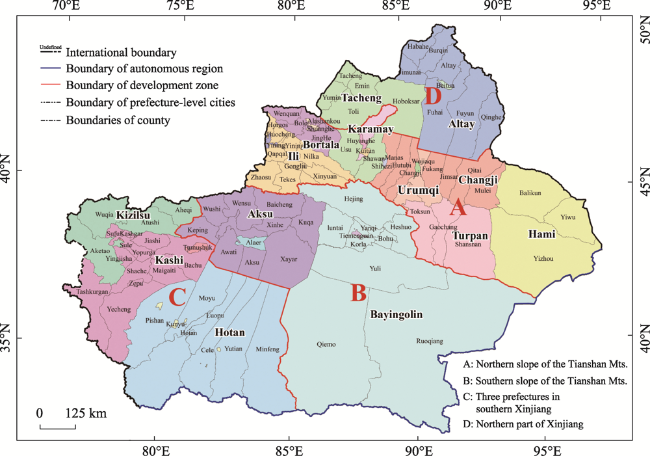
Figure 1 The administrative divisions and regionalization in Xinjiang Uygur Autonomous Region

2.2 Data source

(1) Statistical data
Data on energy consumption, regional GDP, and the total permanent population are available from the Xinjiang Statistical Yearbook 2020. The population data for the whole Xinjiang and its prefectures in 2020 were taken from the public data of the seventh national census. The GDP data for Xinjiang in 2020 were taken from the government work report in 2021. As the population and GDP data of some years in the statistical yearbook were missing, this analysis used interpolation to predict the missing values. For instance, the permanent population size of each prefecture in 2010 and 2019 as well as the GDP data of the city of Shihezi and Aksu Prefecture in 2003 were missing. Considering that the permanent population and GDP ensure good annual continuity and stability, the missing values were estimated using the average GDP of the permanent population in the previous year and that of the permanent population in the following year. Similarly, the missing GDP data of Kashgar Prefecture in 2005-2007 were estimated based on the average annual growth rate of the first five years (1999-2004) and the following five years (2008-2013).
(2) Nighttime light data
This analysis employed the fourth version of the DMSP annual data and the second version of the VIIRS annual data, both of which are available at https://eogdata.mines.edu/products/vnl/. It is noteworthy that the nighttime light value in several counties has been 0 (e.g., Yiwu county during 1992-1999, Wenquan county during 1992-1993, and Aheqi county during 1992-2000). With the application of the trend extrapolation method, this analysis deduces the missing value by calculating the average annual growth rate over the past 10 years.

2.3 Data processing

2.3.1 Synthetic creation and verification of two datasets of nighttime light

In this analysis, we gained nationwide nighttime light data from 1992 to 2020. In our study, the Beijing city has been considered for the verification of the results obtained by previous studies (Wu and Wang, 2019; Ma et al., 2020). The verification results showed the validity of the fitting results.
First, the acquired DMSP annual data needed to be corrected, and the VIIRS annual data needed to be noise-reduced. Second, the VIIRS (2012-2020) and DMSP (2012-2020) datasets overlapped in 2012 and 2013, which is why a sensitivity analysis was performed. The fitted DMSP (2012-2020) dataset was calculated based on the optimal parameters and the VIIRS (2012-2020) annual data, and finally, the “synthetic DMSP” dataset from 1992 to 2020 was obtained.
The linear fitting between the preprocessed VIIRS and DMSP data needed to undergo the following three steps: (1) using a power function to fit the nonlinear relationship between the VIIRS and DMSP datasets; (2) using Gaussian filtering to smoothly fit the DMSP dataset; (3) determining the value range of the fitted DMSP dataset through a set threshold h. The conversion model is shown in formulas (1) and (2):
$Fitted\ DMSP=G(VIIRS,a,b)*M$
$G(X,a,b)=\left( \begin{matrix} ax_{11}^{b} & \cdots & ax_{1n}^{b} \\ \vdots & \ddots & \vdots \\ ax_{m1}^{b} & \cdots & ax_{mn}^{b} \\\end{matrix} \right)$
$M(x,y)=\frac{1}{2\text{ }\!\!\pi\!\!\text{ }{{\sigma }^{2}}}{{e}^{-\frac{({{x}^{2}}+{{y}^{2}})}{2{{\sigma }^{2}}}}}$
As shown in Equation (1), the fitted DMSP was calculated using a transformation function G and a standardized matrix M. Here, * refers to spatial convolution, and the window radius is w. As shown in (2), the transformation function G presents a power function matrix, where xij represents the pixel value of the light data to be converted and located in row i and column j, and a and b are the estimated coefficients. The standardized matrix M represents a Gaussian low-pass filter using a two-dimensional Gaussian kernel function. As shown in Equation (3), the standard deviation σ is the parameter to be estimated.
$fitted\text{ }DMS{{P}_{i,j}}=\left\{ \begin{align} & h\text{ }if\text{ }fitted\text{ }DMS{{P}_{i,j}}>h \\ & fitted\text{ }DMS{{P}_{i,j}} if\text{ }fitted\text{ }DMS{{P}_{i,j}}\le h \\ \end{align} \right.$
By comparing the fitting parameters of Li et al. (2017) and Ma et al. (2020), this analysis chose 63 as the threshold for fitted DMSP data, which is the most consistent with the actual situation of Xinjiang. Then, through the window radius w, the standard deviation σ, and the fitting coefficients a and b, the VIIRS data values are converted into fitted DMSP data according to (1).
The monthly data of DMSP and VIIRS, which have been applied in the study by (Li et al., 2017), has a certain number of overlapping samples (13 months), which is why the cross-validation method was applied for parameter optimization. This analysis used the annual data of the two satellites, and the overlapping years were only 2012 and 2013. Therefore, referring to (Wu and Wang, 2019), this study used sensitive analysis for parameter optimization. The parameter optimization was mainly carried out in four steps. In the beginning, Beijing city was used as a mask to extract the VIIRS (2012–2013) and correct DMSP data during 2012–2013 (Wu and Wang, 2019; Ma et al., 2020). In the first step, referring to (Li et al., 2017), the parameters a and b were set to 11.7319 and 0.4436, respectively. Then, the range of value $\sigma $was set from 0.1 to 5, and it was calculated during every increment of 0.01. The value w ranged from 3 to 50, and it was calculated once in every increment of 2. Among them, the optimal σ and w were determined by calculating the minimum Root Mean Square Error (RMSE) between DMSP data and the fitted DMSP data in Beijing.
$RMSE=\sqrt{\frac{1}{m\times n}\sum\limits_{i=1}^{m}{\sum\limits_{j=1}^{n}{({{x}_{i,j}}-{{{\hat{x}}}_{i,j}})}}}$
The RMSE is shown in Equation (5). xi,j represents the pixel value of the ith row and jth column of the corrected DMSP and ${{\hat{x}}_{i,j}}$ represents the pixel value of the ith row and jth col umn of the fitted DMSP. As shown in Figure 2(1), the first step determined that the optimal σ was 0.95, the optimal w was equal to 3, and the minimum RMSE was equal to 23.7885.
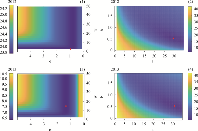
Figure 2 The sensitivity heat map for parameter optimization
In the second step, $\sigma $and w were set to be 0.95 and 3, respectively, as determined in the first step. Simultaneously, the value range of a was defined as 1–35, and it is calculated once in every 0.1 increase; the value range of b was defined as 0.01–2 and was calculated once in every 0.01 increase. The optimal a value is 29.6, the optimal b value is 0.53, and the minimum RMSE is equal to 6.7164, as shown in Figure 2(2).
Using the data from 2013 and repeating the calculation of the first and second steps, the third and fourth steps are followed. Finally, it is determined that the optimal window radius w is 15, the optimal standard deviation is equal to 1.34, and the optimal fitting coefficients a and b were 30.8 and 0.53, respectively. The minimum RMSE was 6.2271, as shown in Figure 2(4).
After using RMSE to measure the effectiveness of the parameters to be estimated, Corr, the Pearson correlation coefficient index, was constructed to test the fitted DMSP. As shown in Equation (6), xi,j represents the pixel value of the ith row and jth column of the corrected DMSP. ${{\hat{x}}_{i,j}}$ represents the pixel value of the ith row and jth column of the fitted DMSP. $\bar{x}$ and $\bar{\hat{x}}$ represents its mean value.
$Corr=\frac{\sum\limits_{i=1}^{m}{\sum\limits_{j=1}^{n}{({{x}_{i,j}}-\bar{x})({{{\hat{x}}}_{i,j}}-\bar{\hat{x}})}}}{\sqrt{\sum\limits_{i=1}^{m}{\sum\limits_{j=1}^{n}{{{({{x}_{i,j}}-\bar{x})}^{2}}}}}\sqrt{\sum\limits_{i=1}^{m}{\sum\limits_{j=1}^{n}{{{({{x}_{i,j}}-\bar{\hat{x}})}^{2}}}}}}$
The RMSE and Corr calculated at each step are shown in Figure 3. Simultaneously, we calculated and compared the RMSE and Corr between DMSP and VIIRS. In 2012 and 2013, the Corr between DMSP and VIIRS was 0.6767 and 0.6753, respectively, and the Corr values between DMSP and fitted DMSP were 0.9851 and 0.9868. Additionally, in 2012 and 2013, RMSEs between DMSP and VIIRS were 37.1351 and 36.9997, and 6.7164 and 6.2271 between DMSP and fitted DMSP.
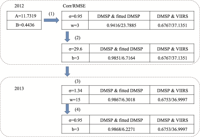
Figure 3 RMSE and Corr coefficients of DMSP and fitted DMSP
The Corr/RMSE coefficients between DMSP and fitted DMSP in 2012 and 2013 calculated by (Wu and Wang, 2019) were 0.937/9.244 and 0.945/9.387, while, here, they are 0.9851/6.7164 and 0.9868/6.2271. The results are a significant improvement over pre-fitting and also more reliable than previous results.
To further verify the reliability of the lighting data, this paper extracted all the raster pixel values of Urumqi, Xinjiang, in two satellite overlapping years (2012 and 2013) and constructed a scatter plot of the two datasets in the same year. The results showed that the fitted DMSP offers a better linear relationship with DMSP than the unfitted VIIRS data (Figure 4).
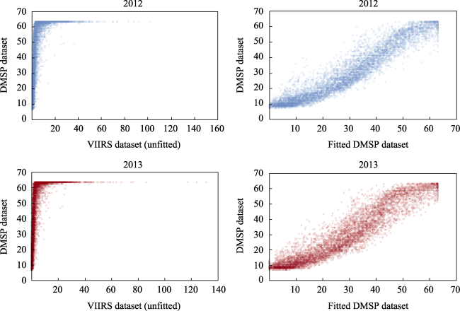
Figure 4 Scatter plots of fitted DMSP and unfitted VIIRS in Urumqi (2012-2013)

2.3.2 Spatialization of carbon emissions

Energy-related carbon emissions were calculated based on the 2006 IPCC Guidelines for National Greenhouse Gas Inventories, which were released by the Intergovernmental Panel on Climate Change (IPCC), and are as follows:
$C{{O}_{2}}=\frac{44}{12}\times \sum\limits_{i=1}^{9}{{{E}_{i}}{{B}_{i}}{{K}_{i}}}$
where CO2 refers to the energy-related carbon emissions with the unit of 104 t, i refers to the category of energy, and Ei refers to the category i’s consumption. The unit of raw coal, coke, crude oil, gasoline, kerosene, diesel, and fuel oil is 104 tons, the unit of natural gas is m3, and of electricity is kWh. Bi refers to the standard coal coefficient of category i. Ki refers to the carbon emission index of category i. The Ki value was derived from the carbon emission calculation guidelines released by the IPCC, and the original unit of J is converted into the standard coal to be consistent with the statistical data unit (1 t standard coal = 29.3 GJ). The standard coal conversion coefficients and carbon emission coefficients of various energy sources are shown in Table 1.
Table 1 Carbon emission factor for different types of fuels
Energy category Coal Coke Crude Gasoline Kerosene Diesel Fuel oil Natural gas Electricity
Standard coal coefficient Bi (tce/t) 0.7143 0.9714 1.4285 1.4714 1.4714 1.4571 1.4286 1.33 0.1229
Carbon emission coefficients Ki (t/tce) 0.7559 0.855 0.5857 0.5538 0.5714 0.5921 0.6185 0.4483 0.272

Note: The unit conversions in electricity are kg/kWh, the unit conversions in natural are kg/m3.

The figure below shows the fit between the total value of nighttime light and carbon emissions. Considering the inversion accuracy of the downscaling model, this paper adopted a linear model without intercepts (Yang et al., 2021b). The results show (as per Equation 8 and Figure 5) that the sum of nighttime lights (SOL) has a good linear correlation with the carbon emission values, which is significantly correlated at 0.01 and R2 = 0.929.
$SOL=0.0262\times C{{O}_{2}}$
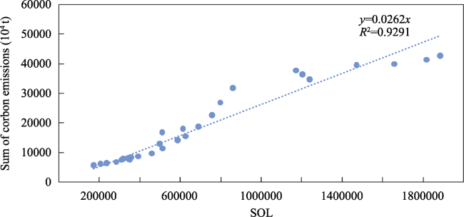
Figure 5 The fitting relationship between SOL and carbon emissions

2.4 Analysis model of spatio-temporal variations in carbon emissions

2.4.1 Calculation of per capita carbon emissions and carbon emission intensity

Using the population and economic statistics of the prefectures, this model analyzed the spatio-temporal distribution of Xinjiang’s per-capita carbon emissions and carbon emission intensity.
$\text{Carbon emission per capita}=\frac{C{{O}_{2}}}{P}$
$\text{Carbon emission intensity}=\frac{C{{O}_{2}}}{GDP}$
where CO2 refers to the sum of carbon emissions, with a unit of 104 t, P refers to the size of the permanent population, with a unit of 104, and GDP refers to the sum of the regional GDPs.

2.4.2 Analysis of carbon emission trends

This study used a univariate linear regression model to analyze the linear tendency (Yang et al., 2021a) and further analyzed the year-on-year change of carbon in each county-level unit. Then, by fitting straight line equation, the slope value (SLOPE) changes from 1992 to 2020 can be calculated as follows:
$SLOPE=\frac{\sum\nolimits_{i=1}^{n}{{{C}_{i}}}\times {{T}_{i}}-({{\sum\nolimits_{i=1}^{n}{C}}_{i}})\times \frac{\sum\nolimits_{i=1}^{n}{{{T}_{i}}}}{n}}{\sum\nolimits_{i=1}^{n}{T_{i}^{2}-\frac{(\sum\nolimits_{i=1}^{n}{{{C}_{i}}{{)}^{2}}}}{n}}}$
where n refers to the total number of years, which is equal to 28, Ti represents the ith year (1992 is the first year), and Ci represents the carbon emissions in the ith year. The larger the SLOPE value, the higher the growth rate of carbon emissions and vice versa.

2.5 Geographical detector

Geographical detector (Wang et al., 2010; Luo et al., 2016; Wang et al., 2016) is used to detect the spatial differentiation, the influencing factors, and the combined interaction among factors influencing carbon emissions in Xinjiang. As a tool, it offers small sample size limitation and easy processing types, among others, and has been applied in many fields of natural and social sciences (Wang et al., 2017c; Ye et al., 2019). This analysis used a geographical detector to detect the significance of each influencing factor on the spatial differentiation of carbon emissions and the combined interaction among factors.
(1) For single-factor detection, significance is measured by the q value, as follows:
$q=1-\frac{\sum\limits_{s=1}^{L}{{{N}_{s}}\sigma _{s}^{2}}}{N{{\sigma }^{2}}}=1-\frac{SSW}{SST}$
where L is the strata (classification) of the variable, Ns and N are the number of units in layer s and the whole region, respectively, $\sigma _{s}^{2}$ and ${{\sigma }^{2}}$ are the variance of carbon emissions within the layer s and the whole region, respectively, and SSW and SST are the sum of squares within the layer and the whole region, respectively. Here, q is the degree of influence for a single factor affecting carbon emissions, with a value range of [0, 1]. The larger the q value, the more this factor explains its influence on carbon emissions and vice versa.
(2) The process of detecting combined interactions is used to assess whether the combination of the two influencing factors will increase or decrease their impact on carbon emissions as compared to their individual influences. The first step is to calculate the q values of the two factors on carbon emissions. The second step is to calculate the q value when the two factors interact (wherein the new polygon distribution is formed by superimposing the two variable layers and resulting tangents).

3 Results

3.1 Simulation accuracy test of carbon emissions

According to the linear function of the SOL and carbon emissions, the spatial distribution map of carbon emissions in Xinjiang on a kilometer grid is generated (Figure 6). To ensure the accuracy and reliability of the simulated carbon emissions, this paper compares them with the carbon emissions in Xinjiang from 1992 to 2020 calculated from statistical data. The results show that the root means square error (RMSE) between the simulated carbon emissions and the statistical data is 3431×104 t and the mean relative error MRE is 13.09%. It can be observed that the carbon emissions simulated based on nighttime light data present good accuracy and can be used to study the characteristics and laws of the spatio-temporal evolution of Xinjiang carbon emissions.
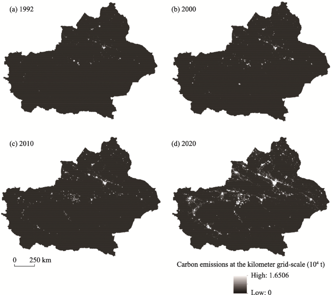
Figure 6 Spatial distribution of carbon emissions at the kilometer grid-scale in Xinjiang

3.2 Spatio-temporal patterns of carbon emissions and Zoning Guidelines for Carbon Reduction

3.2.1 Total carbon emissions and carbon emissions intensity

This section calculates Xinjiang’s carbon emissions based on statistical data. From 1992 to 2020, the total carbon emissions in Xinjiang continued to grow, from 55.57 million tons in 1992 to 427.57 million tons in 2020, with an average annual growth rate of 7.56%. The per-capita carbon emissions have also increased from 3.52 tons/person in 1992 to 16.54 tons/person in 2020, with an average annual growth rate of 5.69%. Carbon emission intensity has been decreasing yearly, from 13.81 tons/10,000 yuan in 1992 to 3.1 tons/10,000 yuan in 2020, with an average annual decrease of 5.2%. Overall, Xinjiang’s carbon emissions have experienced four stages of evolution. (1) The growth rate of carbon emissions from 1992 to 2000 was relatively flat, with an average annual growth rate of 3.68%. (2) From 2000 to 2010, the growth rate of carbon emissions accelerated, with an average annual growth rate of 8.9%. (3) The total carbon emissions from 2010 to 2015 increased rapidly, with an average annual growth rate of 14.24%, indicating an increase of 176.9 million tons in only 5 years and exceeding the increase in carbon emissions over the past 18 years. (4) The growth rate slowed down from 2015 to 2020, with an average annual growth rate of only 3.28%, which was lower than the growth rate before 2000 (Figure 7). At this stage, the overall carbon emissions indicated a trend of convergence, but it still has not peaked.
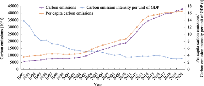
Figure 7 Trends of total carbon emissions and carbon emission intensity changes in Xinjiang

3.2.2 Changing trends in carbon emissions by region

Due to different stages of economic development in each region, carbon emissions, per-capita carbon emissions, and carbon emissions per unit GDP in each region show certain phase differences. The results show that the total carbon emission in descending order is the northern slope of Tianshan > the southern slope of Tianshan > the three prefectures in southern Xinjiang > the northern part of Xinjiang (Figure 8). The per-capita carbon emissions in descending order are the northern part of Xinjiang > southern slope of Tianshan > northern slope of Tianshan > three prefectures in southern Xinjiang (Figure 9). Moreover, carbon emission intensity in descending order is the northern part of Xinjiang > the three prefectures in southern Xinjiang > the southern slope of Tianshan > northern slope of Tianshan (Figure 10).
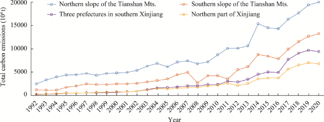
Figure 8 Total carbon emissions of four regions in Xinjiang from 1992 to 2020
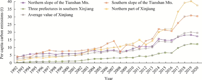
Figure 9 Per capita carbon emissions of four regions in Xinjiang from 1992 to 2020
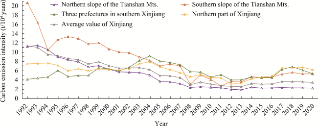
Figure 10 Carbon emission intensity of four regions in Xinjiang from 1992 to 2020
Regarding the first sub-region, the northern slope of Tianshan has the highest population concentration and the most developed economy in Xinjiang. It is also the region with the highest proportion of energy consumption. From 1993 to 1994, its carbon emissions accounted for more than two-thirds of Xinjiang’s total, reaching its highest peak in history. Since then, this value has shown a downward trend, from 67.53% in 1994 to 40.56% in 2020 (Figure 11). During the same period, the proportion of the total GDP in Xinjiang increased slightly, from 61.19% in 1992 to 63.18% in 2020. Carbon emission intensity has declined the most in this region, among the four major sub-regions, from 11.17 tons/10,000 yuan in 1992 to 2.22 tons/10,000 yuan in 2020, which is a decrease of 80.13%. During these 28 years, the per capita carbon emissions have increased by 364%, which is much lower than the increase in the southern slope of Tianshan (603%), the three prefectures in southern Xinjiang (2669%), and the northern part of Xinjiang (2088%). In general, while the population on the northern slope of Tianshan is stable and the GDP is stable and rising, the proportion of carbon emissions continues to decline. This indicates that the overall efficiency of energy utilization is rapidly improving and that the economy on the northern slope of the Tianshan is transforming and developing better energy structures.
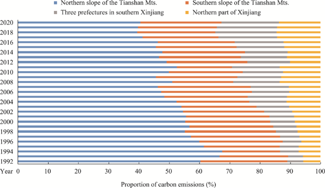
Figure 11 Proportion of carbon emissions of four regions in Xinjiang from 1992 to 2020
Second, the regional carbon emission growth rate of the three prefectures in southern Xinjiang ranks first among the four major regions. Here, carbon emissions rose rapidly from 2.11 million tons in 1992 to 93.7 million tons in 2020, which is an increase of 4350%. Carbon emissions of this region in Xinjiang have also increased from 5.23% in 1992 to 18.98% in 2020. Per-capita carbon emissions increased rapidly from 0.44 tons per capita in 1992 (far below the Xinjiang average of 3.52 tons per capita) to 12.29 tons per capita in 2020, with an increase of 2669% in 28 years. Although per capita carbon emissions are still lower than the Xinjiang average in 2020 (16.54 tons/person), this gap is gradually narrowing. In the past 28 years, the southern Xinjiang region has achieved remarkable results in promoting economic and social development oriented towards bettering people’s livelihoods. The living standards here have been greatly improved, and per-capita energy consumption has also rapidly increased. However, it is worth observing that the carbon emission intensity of the three prefectures in southern Xinjiang has demonstrated a fluctuating upward trend in the past 28 years, rising from 4.13 tons/10,000 yuan in 1992 to 5.36 tons/10,000 yuan in 2020. This shows that the efficiency of energy utilization in southern Xinjiang is not high and that the overall economic development benefits need to be further improved.
Third, carbon emissions in the southern slope of Tianshan increased from 11.58 million tons in 1992 to 132.01 million tons in 2020, with an increase of 1040%. In terms of the proportion of total carbon emissions in Xinjiang, it accounted for 28.74% in 1992 and 26.74% in 2020. Per-capita carbon emissions increased from 4.34 tons/person in 1992 to 30.5 tons/person in 2020, which is an increase of 603% in 28 years. Carbon emission intensity has shown a rapid downward trend, from 20.67 tons/10,000 yuan in 1992 to 5.24 tons/10,000 yuan in 2020, with a drop of 74.48%, second only to the northern slope of Tianshan. This shows that the energy efficiency of the region is improving rapidly.
Finally, carbon emissions in northern Xinjiang increased from 2.3 million tons in 1992 to 67.74 million tons in 2020, which is an increase of 2847% and second only to the three prefectures in southern Xinjiang. The proportion of total carbon emissions in Xinjiang it accounted for has increased, from 5.71% in 1992 to 13.72% in 2020. Per-capita carbon emissions have increased rapidly from 1.71 tons/person in 1992 (which is also lower than the average of 3.52 tons/person in Xinjiang) to 37.48 tons/person in 2020, which is considerably higher than the Xinjiang average for the same period (16.54 tons/person). Additionally, the growth rate reached 2088% in 28 years. The overall carbon emission intensity demonstrates a fluctuating downward trend, but this is not obvious. From 7.44 tons per 10,000 yuan in 1992 to 6.23 tons per 10,000 yuan in 2020, a decline of 16.22% can be observed, which is far lower than the Xinjiang average (69.96%). Moreover, carbon emission intensity in 2020 is much higher than the average value in Xinjiang, indicating that the energy efficiency of northern Xinjiang needs to be further improved.

3.2.3 Change trend of carbon emissions by county and city

Based on nighttime light data, the spatial distribution of carbon emissions on a kilometer grid-scale in Xinjiang was calculated. Figure 12 displays the changes in total carbon emissions of county-level units from 1992 to 2020. Additionally, this analysis uses the trend analysis method to calculate the total carbon emissions of all counties and cities in Xinjiang from 1992 to 2020. It also uses the Jenks Natural Breaks Classification method in ArcGIS to divide the total carbon emissions growth trends of the counties and cities into five types. The five types include low growth, medium-low growth, medium growth, medium-high growth, and high growth, as shown in Figure 13. Specifically, there are 5 counties and cities in Xinjiang that are of high-growth type, namely the counties of Kuqa and Xayar and cities of Urumqi, Karamay, and Yizhou. Further, 15 counties and cities, including Hutubi, Manas, Fukang, Jimsar, Qitai, Toksun, Shawan, Yining, Baicheng, and Wensu counties and Changji, Turpan, Usu, Korla, and Aksu cities, belong to the medium-high growth type. The commonality between these cities and counties is that they are either within the Urban agglomeration on the northern slope of Tianshan or central cities with relatively active economies located on the southern slope of the Tianshan. Twenty other counties and cities, which are relatively lagging in economic development, belong to the medium growth type. Moreover, 34 counties and cities belong to the medium-low growth type, while 22 counties and cities belong to the slow growth type, which are located far away from the central city and relatively lagging in economic development.
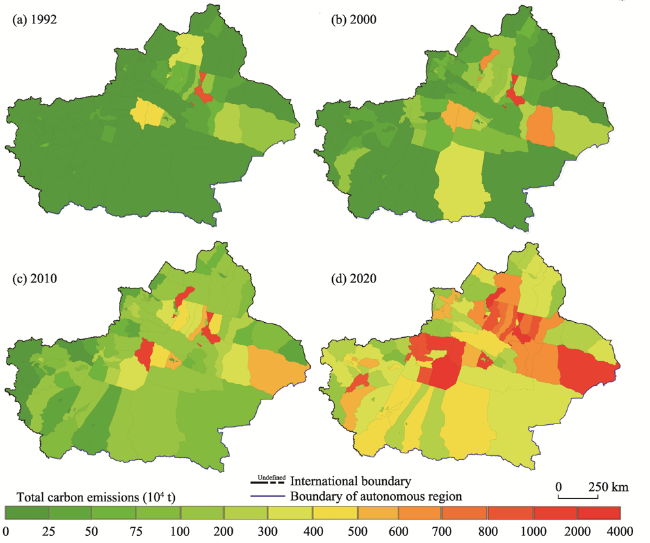
Figure 12 Spatio-temporal distribution of total carbon emissions in Xinjiang from 1992 to 2020
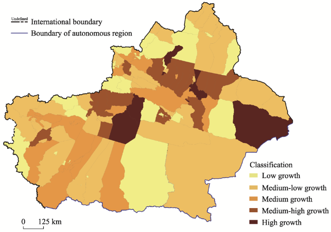
Figure 13 Classification of carbon emissions increment speeds in Xinjiang from 1992 to 2020
A closer look at the history of economic development in developed countries reveals that the relationship between the stage of the development and carbon emissions has four stages. The first stage is characterized by low per-capita income and low carbon emission intensity. In comparison, there is low per-capita income and high carbon emission intensity in the second stage. The third has high per-capita income and high carbon emission intensity, while the fourth stage has high per-capita income and low carbon emission intensity. With the average emission levels of Xinjiang as the origin of the two-dimensional coordinate axis (the carbon emission intensity per unit of GDP is 3.1 tons per 10,000 yuan and the per-capita GDP is 55,000 yuan), this analysis distributed the data into four quadrants. The distribution map formed by placing all counties and cities in Xinjiang into corresponding quadrants is shown in Figure 14. The following four observations were made.
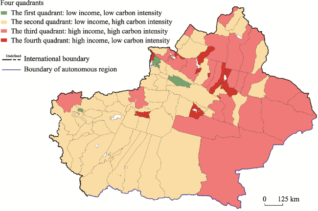
Figure 14 Four quadrants of per-capita GDP and carbon intensity
First, there were nine counties in the fourth quadrant with high per-capita income and low carbon emission intensity. These cities were the first batch of cities in Xinjiang to start industrialization (such as Urumqi, Karamay, Changji, Korla, and Kuitun) and port cities (such as Alashankou city and Horgos city). From the political perspective, it is suggested that such cities play a leading role in carbon emission reduction in Xinjiang and promote regional innovation reform, the conversion of new and old kinetic energy, and the optimization and upgrading of industries. By developing high-tech, modern service and modern agricultural industries, the nine cities are expected to reduce the carbon emission intensity per unit of GDP and take the lead in achieving carbon peaking.
There were 23 cities in the third quadrant, which were characterized by relatively high per-capita income and high carbon emission intensity. These cities are currently in the stage of rapid industrialization, and the heavy chemical industry accounts for a high proportion. Two aspects of development-related policy are proposed to achieve the dual-carbon goal in an orderly manner. On one hand, it is necessary to reserve a certain space for carbon emissions considering their developmental stage. On the other hand, the existing heavy chemical industry is suggested to improve energy efficiency by technological upgrading and orderly exit of the backward industries that have high energy consumption and low efficiency.
There were 53 cities in the second quadrant, which were characterized by relatively low per-capita income and high carbon emission intensity. These cities are mainly distributed in the Aksu region, Kyzilsu Kirgiz Autonomous Prefecture, Kashgar region, Hotan region, and counties that are directly under Yili Kazak Autonomous Prefecture. The common characteristic of these cities is that they are currently in the early stage of industrialization and the industrial foundation is relatively weak. They have just completed poverty alleviation and, hence, are eager to develop labor-intensive industries to provide sufficient jobs in the long future. Therefore, such cities should focus on accelerating urbanization and industrialization levels, improving people’s living standards, and narrowing the gap with the average level of Xinjiang. Therefore, it is recommended to formulate carbon emission reduction policies such as optimizing energy structure, adjusting the industrial structure, and improving economic benefits, which are in line with the development stage.
There were four cities in the first quadrant (Kashgar city, Yining city, Huocheng county, and Xinyuan county) with low-income and low-carbon emission intensity. These cities are dominated by light industry, agriculture and animal husbandry, and tourism. It is noteworthy that these cities are ecologically sensitive areas in Xinjiang. For these cities, consideration must be given to ecological security systems, employment security, social welfare, and public services. Therefore, it is recommended to strengthen ecological compensation and financial transfer payments.
In sum, 85% of the cities were present in the second and third quadrants, indicating that most cities have high carbon intensity and that economic benefits of carbon emissions need to be improved.

3.3 Analysis of influencing factors

With the application of a geographical detector, this paper analyzes factors from five aspects and seven indicators of carbon emissions. The first aspect is economic growth, for which GDP and the scale of the output value of the secondary industry (SV) were selected as the indicators. The second aspect is the population size, for which the population size (POP) was selected as the indicator. The third aspect is the urbanization level, for which the urbanization rate (UR) and the size of the urban population (UP) were selected as indicators. The fourth aspect is the industrial structure, and its indicators include the proportion of the secondary industry in GDP (SP). The fifth aspect is the energy consumption intensity, and energy consumption intensity per unit of GDP (EIG) is selected as the indicator. The dataset at the county-level unit in the years 1992, 2000, 2010, and 2020 was constructed. This is followed by the classification of the factors with the application of the Jenks Natural Breaks Classification method in ArcGIS. The contribution and results of the interaction of each factor with carbon emissions are shown in Tables 2 and 3.
Table 2 Detection results for influencing factors
Influencing factor Index q
1992 2000 2010 2020
Economic growth Gross Domestic Product (GDP) 0.654*** 0.685*** 0.746*** 0.431*
The secondary industry output value (SV) 0.564*** 0.612*** 0.672*** 0.440***
Industrial structure The ratio of secondary industry output value to GDP (SP) 0.211** 0.352*** 0.215*** 0.133**
Population size Population size (POP) 0.517** 0.420 0.462* 0.398*
Urban population size (UP) 0.529** 0.571*** 0.562*** 0.391*
Urbanization level Urbanization rate (UR) 0.115* 0.313*** 0.258*** 0.197**
Energy consumption intensity Energy consumption intensity per unit of GDP (EIG) 0.354*** 0.205* 0.268 0.378*

Note: *0.05<p<0.1; **0.01< p <0.05; *** p <0.01

Table 3 Detection results of interaction for influencing factors
Interacting factors 1992 Interacting factors 2000 Interacting factors 2010 Interacting factors 2020
GDP∩EIG 0.990 SV∩EIG 0.934 GDP∩EIG 0.942 SV∩EIG 0.869
POP∩EIG 0.905 GDP∩EIG 0.918 SV∩EIG 0.857 GDP∩EIG 0.860
SV∩EIG 0.879 POP∩SP 0.782 SV∩UR 0.830 UP∩ EIG 0.789
UP∩ EIG 0.866 UP∩SP 0.777 GDP∩UR 0.816 POP∩EIG 0.777
POP∩GDP 0.798 POP∩SV 0.768 SV∩UP 0.813 UR∩ EIG 0.616
POP∩SP 0.714 UP∩ EIG 0.768 POP∩SV 0.811 UR∩ POP 0.602
GDP∩SP 0.709 SV∩UP 0.746 GDP∩SP 0.794 POP∩SP 0.583
SV∩SP 0.701 SV∩UR 0.733 SV∩SP 0.793 UR∩ SV 0.582
GDP∩POP 0.674 GDP∩SP 0.749 GDP∩POP 0.774 SV∩UP 0.544
GDP∩SV 0.673 GDP∩POP 0.724 UR∩POP 0.757 SV∩POP 0.543

3.3.1 Detection of a single factor

(1) Economic growth. The scale of economic growth offers the most significant explanatory power for the spatial differentiation of carbon emissions, and it shows a trend of first increasing and then decreasing. The q values of the GDP in 1992 and 2010 were 0.65and 0.75, respectively, indicating that GDP was among the most explanatory factors in 1992 and 2010. Then, in 2020, the value dropped to 0.43, indicating that GDP’s explanatory power for the spatial differentiation of carbon emissions declined. As for the output value of the secondary industry (SV), the changing trend of the explanatory power of the output value of the secondary industry, regarding the spatial differentiation of carbon emissions is consistent with that of the GDP. The q values in 1992 and 2000 were 0.56 and 0.67, respectively and dropped to 0.44 in 2020. This indicates that, before 2010, there was a strong correlation between carbon emissions and economic size, and the growth of carbon emissions was mainly driven by the increase in economic growth. However, after 2010, the carbon emission intensity of some cities began to decline, indicating that the rapid economic growth did not bring about the simultaneous growth of carbon emissions. In the northern slope of Tianshan, it was observed that the proportion of GDP increased while the proportion of carbon emissions decreased, also showing that the overall economic development and energy efficiency of some areas in the northern slope of Tianshan has been continuously improving.
(2) The influence of the proportion of the secondary industry on GDP (SP) is relatively weak in explaining the spatial differentiation of carbon emissions. The q values of the four years studied were 0.21, 0.35, 0.21, and 0.13, respectively, which indicated that the overall value is relatively low and displayed a downward trend.
(3) The explanatory power of the population size for the spatial differentiation of carbon emissions showed a strong as well as relatively stable trend. The q values in the four years range from 0.4 to 0.52, implying that the population size has significant explanatory power for the spatial differentiation of carbon emissions. This is because energy-related carbon emissions at this stage are closely related to people’s production and living needs. Besides, the q value of the level of urbanization in the years 1992, 2000, 2010, and 2020 was low, indicating that the urbanization rate has been generally weak in explaining the spatial differentiation of carbon emissions. Meanwhile, the explanatory power of urban population size on the spatial differentiation of carbon emissions is very significant. This demonstrates that the impact of the level of urbanization on the spatial differentiation of carbon emissions is primarily driven by the increase in energy consumption resulting from the expansion of the urban population, which, in turn, promotes an increase in carbon emissions. This is consistent with the influence mechanism of population size on the spatial differentiation of carbon emissions. The urbanization rate has no significant impact on the spatial differentiation of carbon emissions because there are extremely large gaps in the population size of various prefectures in Xinjiang. Therefore, prefectures with high urbanization rates are not necessarily regions with large urban populations. Therefore, the urbanization rate cannot explain the spatial differentiation of total carbon emissions.
(4) Energy consumption intensity per unit of GDP (EIG) has significant explanatory power for the spatial differentiation of carbon emissions, and fluctuated between 0.2 and 0.38. It shows that the impact of energy utilization efficiency on carbon emissions cannot be ignored. Cities can improve energy utilization efficiency by technological upgrading and optimizing industrial structure optimization, thereby accelerating the process of carbon emission reduction.

3.3.2 Detecting interactions

In this section, the top 10 interaction influencing factors across the four years under study have been summarized in Table 3. The results demonstrated that the interactions between various factors have significantly increased. Three observations can be made: (1) The ratio of the secondary industry (SP) and the urbanization rate (UR), two indicators that reflect the “structural scale effect” have low individual q values. However, when they interacted with other factors that can reflect the “scale effect” (such as GDP, POP), the q values increased greatly. For instance, the q value of the interactions between SP and GDP reached 0.709, 0.749, and 0.794 in 1992, 2000, and 2010, respectively. The q value of interactions between UR and POP reached 0.757 and 0.602 in 2010 and 2010. (2) As the factors reflecting economic growth interact with the factors reflecting the population size, the q value increases significantly. For example, the q value of the interactions between GDP and POP in 1992, 2000, and 2010 reached 0.674, 0.724, and 0.774, respectively. (3) The index of EIG has a high q value when it interacts with the economy. For instance, the q value of the interactions between GDP and EIG in 1992, 2000, 2010, and 2020 reached 0.990, 0.918, 0.942, and 0.860, respectively. Further, the q values of the interactions between SV and EIG in 1992, 2000, 2010, and 2020 reached 0.879, 0.934, 0.857, and 0.869, respectively. This suggests that energy consumption intensity, along with economic growth and population size have become important factors of the spatial differentiation of carbon emissions.

4 Discussion and conclusions

4.1 Discussion

Although the use of nighttime light data can invert the spatio-temporal variations in regional carbon emissions within a certain time, there uncertainties in the following aspects. First, cross-regional power transmission may cause a deviation of carbon emission inversion. For instance, in a city that uses electricity input from outside the district as its primary energy source, its carbon emissions’ estimates based on the brightness of nighttime lights may be relatively high. Second, the increase in the proportion of new energy consumption such as wind, solar, and nuclear energy may lead to deviations in the inversion of carbon emissions. Moreover, the higher the proportion of new energy consumption, the greater the deviation of carbon emissions estimates based on the brightness of nighttime lights. Finally, the increase in the brightness values of the nighttime lights is approximately linear, and the carbon emissions show a trend of first increasing and then decreasing with increasing economic growth.
Therefore, with economic and social development and technological progress, there is a “decoupling” phenomenon between the brightness of nighttime lights and carbon emissions. As previous studies have indicated, this is due to the decoupling of carbon emissions and economic growth. It must be noted that using nighttime light data to carry out carbon emissions inversion over a long study duration may lead to deviations in simple linear simulations. Further, the longer the period, the more obvious the deviations. As such, the above viewpoints need to be further verified by empirical research.

4.2 Conclusions

This analysis attempts to integrate two datasets of nighttime light, DMSP/OLS and NPP/VIIRS, to construct a “synthetic DMSP” dataset from 1992 to 2020. By calculating the total carbon emissions over the years using Xinjiang energy consumption statistics, this analysis establishes the functional relationship between energy consumption, carbon emissions, and the total value of nighttime lights. The fitting results show that the sum of nighttime lights (SOL) shares a good linear correlation with the carbon emissions. Therefore, the spatio-temporal variations in Xinjiang’s total carbon emissions can be better inverted through the nighttime light. On this basis, this analysis used the geographical detector method to analyze the degree of influence of factors such as economic growth, population size, urbanization level, industrial structure, and industrial energy consumption. The primary findings are as follows.
(1) From 1992 to 2020, the total carbon emissions in Xinjiang continued to grow, from 55.57 million tons in 1992 to 427.57 million tons in 2020. The average annual growth rate increased rapidly from 3.68% in 1992-2000 to 14.24% in 2010-2015. The growth rate from 2015 to 2020 was 3.28%, which implies that the growth rate has declined. Per-capita carbon emissions have also increased from 3.52 tons/person in 1992 to 16.54 tons/person in 2020, with an average annual growth rate of 5.69%. Carbon emission intensity reduced from 13.81 tons/10,000 yuan in 1992 to 3.1 tons/10,000 yuan in 2020, with an average annual decrease of 5.2%. In conclusion, Xinjiang’s carbon emissions display a trend of convergence, but they have not peaked.
(2) There are large regional differences in Xinjiang’s total carbon emissions, per-capita carbon emissions, and carbon emissions intensity. The area on the northern slope of Tianshan has always generated the largest carbon emissions as a result of energy consumption in Xinjiang. However, from 1992 to 2020, while the population remained stable and the GDP rose steadily, the proportion of carbon emissions in the region continued to decline in the whole Xinjiang. This shows that the overall energy utilization efficiency of the northern slope of Tianshan is rapidly improving, and it is developing better energy structures. The proportion of regional carbon emissions in the three prefectures in southern Xinjiang has risen rapidly, and the gap between per-capita carbon emissions and the average level of Xinjiang has gradually narrowed. The rapid improvement of the standard of living in this region has brought about a simultaneous increase in per-capita energy consumption. Unlike other three regions, carbon emission intensity in this region has not decreased but increased, indicating that it is still in the extensive development stage of inefficient energy use. The proportion of carbon emissions in the southern slope of Tianshan in Xinjiang is relatively stable, carbon emission intensity shows a rapid downward trend, and the overall energy utilization efficiency is rapidly improving. The proportion of carbon emissions in the northern part of Xinjiang continues to increase, per-capita carbon emissions have increased rapidly, and carbon emissions intensity has slowly declined. This shows that the northern part of Xinjiang is still in the development stage of high energy consumption and high carbon emissions.
(3) At the county level, the high-growth counties (districts) include Urumqi, Karamay, Yizhou district in Hami, Kuqa city and Xayar county in Aksu, which are the capitals of autonomous regions or prefectures with strong populations and attractive economies. The 15 medium-high growth cities are either within the urban agglomeration on the northern slope of Tianshan or central cities with relatively active economies located in the southern slope of Tianshan. The other 20 counties and cities, which are relatively lagging in economic development, belong to the medium growth type. Further, 34 counties and cities belong to the medium-low growth type, while 22 counties and cities belong to the slow growth type and are located far away from the central city and relatively lagging in economic development.
(4) Based on their stage of economic development and the characteristics of carbon emission intensity, this analysis divided the cities in Xinjiang into the following four categories: 1) low per-capita income and low carbon emission intensity, 2) low per-capita income and high carbon emission intensity, 3) high per-capita income and high carbon emission intensity, and 4) high per-capita income and low carbon emission intensity. This analysis proposes to formulate differentiated carbon emission reduction targets and strategies according to the economic development stage and carbon intensity characteristics of each city, to promote each city to achieve the carbon peak goal batch-wise, in an orderly manner.
(5) Results obtained by the geographical detector technique showed that economic growth, population size, and energy consumption intensity are the main influencing factors for the spatial differentiation of carbon emissions. Economic growth offers the most significant explanatory power, and its explanatory power increases and then decreases. The explanatory power of population size on the spatial differentiation of carbon emissions is second only to economic size and is relatively stable. The impact of energy intensity on the spatial differentiation of carbon emissions is also significant. The ratio of the secondary industry and the urbanization rate, the two indicators that reflect the “structural scale effect,” have low individual q values. However, when they interact with other factors that can reflect the “scale effect”, the q values increase greatly. Interactions between economic growth and population size and the interaction between economic growth and energy consumption intensity also significantly enhance the explanatory power of the spatial differentiation of carbon emissions, indicating that the spatial differentiation of carbon emissions among counties and cities is mainly driven by economic growth, population size, and energy consumption intensity.
[1]
Chen J, Gao M, Cheng S et al., 2020. County-level CO2 emissions and sequestration in China during 1997-2017. Scientific Data, 7(1): 1-12.

DOI

[2]
Cui C, Shan Y, Liu J et al., 2019. CO2 emissions and their spatial patterns of Xinjiang cities in China. Applied Energy, 252: 113473.

DOI

[3]
Elvidge C D, Baugh K, Zhizhin M et al., 2017. VIIRS night-time lights. International Journal of Remote Sensing, 38(21): 5860-5879.

DOI

[4]
Friedlingstein P, O'Sullivan M, Jones M W et al., 2020. Global Carbon Budget 2020. Earth System Science Data, 12(4): 3269-3340.

DOI

[5]
Guan D, Hubacek K, Weber C L et al., 2008. The drivers of Chinese CO2 emissions from 1980 to 2030. Global Environmental Change, 18(4): 626-634.

DOI

[6]
Han M, Yao Q, Lao J et al., 2020. China’s intra- and inter-national carbon emission transfers by province: A nested network perspective. Science China Earth Sciences, 63(6): 852-864.

DOI

[7]
Han M, Yao Q, Liu W et al., 2018. Tracking embodied carbon flows in the Belt and Road regions. Journal of Geographical Sciences, 28(9): 1263-1274.

DOI

[8]
Hausfather Z, Peters G P, 2020. Emissions: The ‘business as usual’ story is misleading. Nature, 577(7792): 618-620.

DOI

[9]
Li X, Li D, Xu H et al., 2017. Intercalibration between DMSP/OLS and VIIRS night-time light images to evaluate city light dynamics of Syria’s major human settlement during Syrian Civil War. International Journal of Remote Sensing, 38(21): 5934-5951.

DOI

[10]
Liu Y, Yan B, Zhou Y, 2016. Urbanization, economic growth, and carbon dioxide emissions in China: A panel cointegration and causality analysis. Journal of Geographical Sciences, 26(2): 131-152.

DOI

[11]
Liu Z, Guan D, Moore S et al., 2015a. Climate policy: Steps to China’s carbon peak. Nature, 522(7556): 279-281.

DOI

[12]
Liu Z, Guan D, Wei W et al., 2015b. Reduced carbon emission estimates from fossil fuel combustion and cement production in China. Nature, 524(7565): 335-338.

DOI

[13]
Liu Z, He C, Zhang Q et al., 2012. Extracting the dynamics of urban expansion in China using DMSP-OLS nighttime light data from 1992 to 2008. Landscape and Urban Planning, 106(1): 62-72.

DOI

[14]
Luo W, Jasiewicz J, Stepinski T et al., 2016. Spatial association between dissection density and environmental factors over the entire conterminous United States. Geophysical Research Letters, 43(2): 692-700.

DOI

[15]
Ma J, Guo J, Ahmad S et al., 2020. Constructing a new inter-calibration method for DMSP-OLS and NPP-VIIRS nighttime light. Remote Sensing, 12(6): 937.

DOI

[16]
Meng L, Graus W, Worrell E et al., 2014. Estimating CO2 (carbon dioxide) emissions at urban scales by DMSP/OLS (Defense Meteorological Satellite Program’s Operational Linescan System) nighttime light imagery: Methodological challenges and a case study for China. Energy, 71: 468-478.

DOI

[17]
Mi Z, Meng J, Guan D et al., 2017. Chinese CO2 emission flows have reversed since the global financial crisis. Nature Communications, 8(1): 1-10.

DOI

[18]
Shan Y, Fang S, Cai B et al., 2021. Chinese cities exhibit varying degrees of decoupling of economic growth and CO2 emissions between 2005 and 2015. One Earth, 4(1): 124-134.

DOI

[19]
Shan Y, Liu J, Liu Z et al., 2019. An emissions-socioeconomic inventory of Chinese cities. Scientific Data, 6: 190027.

DOI

[20]
Shi K, Chen Y, Yu B et al., 2016. Detecting spatiotemporal dynamics of global electric power consumption using DMSP-OLS nighttime stable light data. Applied Energy, 184: 450-463.

DOI

[21]
Su W, Liu Y, Wang S et al., 2018. Regional inequality, spatial spillover effects, and the factors influencing city-level energy-related carbon emissions in China. Journal of Geographical Sciences, 28(4): 495-513.

DOI

[22]
Su Y, Chen X, Li Y et al., 2014. China’s 19-year city-level carbon emissions of energy consumptions, driving forces and regionalized mitigation guidelines. Renewable and Sustainable Energy Reviews, 35: 231-243.

DOI

[23]
Su Y, Chen X, Wang C et al., 2015. A new method for extracting built-up urban areas using DMSP-OLS nighttime stable lights: A case study in the Pearl River Delta, southern China. Giscience & Remote Sensing, 52(2): 218-238.

[24]
Wang C, Miao Z, Chen X et al., 2021. Factors affecting changes of greenhouse gas emissions in Belt and Road countries. Renewable and Sustainable Energy Reviews, 147: 111220.

DOI

[25]
Wang C, Wang F, Zhang H et al., 2014. China’s carbon trading scheme is a priority. Environmental Science & Technology, 48(23): 13559-13559.

DOI

[26]
Wang C, Wang F, Zhang X et al., 2017a. Examining the driving factors of energy related carbon emissions using the extended STIRPAT model based on IPAT identity in Xinjiang. Renewable and Sustainable Energy Reviews, 67: 51-61.

DOI

[27]
Wang C, Wang F, Zhang X et al., 2017b. Influencing mechanism of energy-related carbon emissions in Xinjiang based on the input-output and structural decomposition analysis. Journal of Geographical Sciences, 27(3): 365-384.

DOI

[28]
Wang C, Zhang H, Wang F et al., 2019a. Slash local emissions to protect Tibetan Plateau. Nature, 566(7745): 455.

[29]
Wang J, Lu F, 2021. Modeling the electricity consumption by combining land use types and landscape patterns with nighttime light imagery. Energy, 234: 121305.

DOI

[30]
Wang J F, Li X H, Christakos G et al., 2010. Geographical detectors-based health risk assessment and its application in the neural tube defects study of the Heshun region, China. International Journal of Geographical Information Science, 24(1): 107-127.

DOI

[31]
Wang J F, Zhang T L, Fu B J, 2016. A measure of spatial stratified heterogeneity. Ecological Indicators, 67: 250-256.

DOI

[32]
Wang S, Gao S, Huang Y et al., 2020a. Spatiotemporal evolution of urban carbon emission performance in China and prediction of future trends. Journal of Geographical Sciences, 30(5): 757-774.

DOI

[33]
Wang S, Huang Y, Zhou Y, 2019b. Spatial spillover effect and driving forces of carbon emission intensity at the city level in China. Journal of Geographical Sciences, 29(2): 231-252.

DOI

[34]
Wang S, Liu X, 2017. China’s city-level energy-related CO2 emissions: Spatiotemporal patterns and driving forces. Applied Energy, 200: 204-214.

DOI

[35]
Wang Y, Li G, 2017. Mapping urban CO2 emissions using DMSP/OLS ‘city lights’ satellite data in China. Environment and Planning A: Economy and Space, 49(2): 248-251.

DOI

[36]
Wang Y, Liu Z, He C et al., 2020b. Quantifying urbanization levels on the Tibetan Plateau with high-resolution nighttime light data. Geography and Sustainability, 1(3): 233-244.

DOI

[37]
Wang Y, Wang S, Li G et al., 2017c. Identifying the determinants of housing prices in China using spatial regression and the geographical detector technique. Applied Geography, 79: 26-36.

DOI

[38]
Wei Y, Liu H, Song W et al., 2014. Normalization of time series DMSP-OLS nighttime light images for urban growth analysis with pseudo invariant features. Landscape and Urban Planning, 128: 1-13.

DOI

[39]
Welsby D, Price J, Pye S et al., 2021. Unextractable fossil fuels in a 1.5 °C world. Nature, 597(7875): 230-234.

DOI

[40]
Wu K, Wang X, 2019. Aligning pixel values of DMSP and VIIRS nighttime light images to evaluate urban dynamics. Remote Sensing, 11(12): 1463.

DOI

[41]
Yang Y, Wu J, Wang Y et al., 2021a. Quantifying spatiotemporal patterns of shrinking cities in urbanizing China: A novel approach based on time-series nighttime light data. Cities, 118: 103346.

DOI

[42]
Yang Z, Chen Y, Guo G et al., 2021b. Using nighttime light data to identify the structure of polycentric cities and evaluate urban centers. Science of the Total Environment, 780: 146586.

DOI

[43]
Ye Y, Wu K, Xie Y et al., 2019. How firm heterogeneity affects foreign direct investment location choice: Micro-evidence from new foreign manufacturing firms in the Pearl River Delta. Applied Geography, 106: 11-21.

DOI

[44]
Zhang Y, Pan J, Zhang Y et al., 2021. Spatial-temporal characteristics and decoupling effects of China’s carbon footprint based on multi-source data. Journal of Geographical Sciences, 31(3): 327-349.

DOI

Outlines

/