Uncovering differences in the spatial structure of intercity interactive networks described by multi-source migration flow: From the multi-hierarchical perspective

WEI Shimei; PAN Jinghu

doi:10.1007/s11442-025-2358-8

2025 , Vol. 35 >Issue 5: 1049 - 1079

DOI: https://doi.org/10.1007/s11442-025-2358-8

Special Issue: River Basin and Human Activity

Uncovering differences in the spatial structure of intercity interactive networks described by multi-source migration flow: From the multi-hierarchical perspective

WEI Shimei ,
PAN Jinghu ^,^*

Expand

College of Geography and Environmental Science, Northwest Normal University, Lanzhou 730070, China

*Pan Jinghu (1974-), PhD and Professor, specialized in spatial analysis and perception. E-mail: panjh_nwnu@nwnu.edu.cn

Wei Shimei (1993-), PhD, specialized in spatial analysis and perception. E-mail: 2020120156@nwnu.edu.cn

Received date: 2024-05-30

Accepted date: 2025-01-23

Online published: 2025-09-05

Supported by

National Natural Science Foundation of China(42361040)

Fold

Abstract

Population migration data derived from location-based services has often been used to delineate population flows between cities or construct intercity relationship networks to reveal and explore the complex interaction patterns underlying human activities. Nevertheless, the inherent heterogeneity in multimodal migration big data has been ignored. This study conducts an in-depth comparison and quantitative analysis through a comprehensive lens of spatial association. Initially, the intercity interactive networks in China were constructed, utilizing migration data from Baidu and AutoNavi collected during the same time period. Subsequently, the characteristics and spatial structure similarities of the two types of intercity interactive networks were quantitatively assessed and analyzed from overall (network) and local (node) perspectives. Furthermore, the precision of these networks at the local scale is corroborated by constructing an intercity network from mobile phone (MP) data. Results indicate that the intercity interactive networks in China, as delineated by Baidu and AutoNavi migration flows, exhibit a high degree of structure equivalence. The correlation coefficient between these two networks is 0.874. Both networks exhibit a pronounced spatial polarization trend and hierarchical structure. This is evident in their distinct core and peripheral structures, as well as in the varying importance and influence of different nodes within the networks. Nevertheless, there are notable differences worthy of attention. Baidu intercity interactive network exhibits pronounced cross-regional effects, and its high-level interactions are characterized by a “rich-club” phenomenon. The AutoNavi intercity interactive network presents a more significant distance attenuation effect, and the high-level interactions display a gradient distribution pattern. Notably, there exists a substantial correlation between the AutoNavi and MP networks at the local scale, evidenced by a high correlation coefficient of 0.954. Furthermore, the “spatial dislocations” phenomenon was observed within the spatial structures at different levels, extracted from the Baidu and AutoNavi intercity networks. However, the measured results of network spatial structure similarity from three dimensions, namely, node location, node size, and local structure, indicate a relatively high similarity and consistency between the two networks.

Key words： network differences; interactive network; intercity migration; multimodal data; China

Cite this article

WEI Shimei , PAN Jinghu . Uncovering differences in the spatial structure of intercity interactive networks described by multi-source migration flow: From the multi-hierarchical perspective[J]. Journal of Geographical Sciences, 2025 , 35(5) : 1049 -1079 . DOI: 10.1007/s11442-025-2358-8

1 Introduction

Since the beginning of the 21st century and the subsequent rise of the Internet era, the continuous rise across various industries has given birth to the generation of substantial volumes of novel spatiotemporal big data (Fan et al., 2014). The emergence and application of big data with high spatiotemporal accuracy provides new opportunities and perspectives for a deeper understanding of regional development, spatial interaction and the impacts of major public safety events (Haraguchi et al., 2022; Wang et al., 2024). This not only enhances our comprehension of geospatial dynamics but also supports swift decision-making and innovation across various fields. However, despite serving as a foundation for numerous studies on human-land relationships, the quality of intercity migration data remains inconsistent, affected by factors such as varied sources, diverse structures, and differing statistical standards. For instance, population mobility data released by major internet corporations (such as Google, Alibaba, Baidu) and mobile phone communication operators may exhibit deviations and one-sidedness owing to their respective user sample coverage, focus, statistical techniques (Shi et al., 2018), thereby offering a limited perspective that could potentially distort interpretations of urban spatial interactions. Accordingly, the verification and comparison of data are crucial premises, particularly in the context of frequent public safety events. In addition, dependence on biased big data for decision-making may cause unforeseen and unnecessary risks.

Investigating the structure of intercity interactive networks from the perspective of “space of flows” can provide valuable insights into the association relationships, hierarchical features, and spatial organization patterns between cities (Castells, 1996; Pan and Lai, 2019; Ye and Qian, 2021; Zhao and Gao, 2024). The perspective considers the dynamic exchanges of information, goods, and individuals, rather than static geographical locations, to understand the functional relationships and mutual influences among cities (Yang et al., 2022; Zhou et al., 2024b). However, many existing studies on the characteristics of intercity relationship networks rely on a single data source, such as statistical survey data (Gao et al., 2023), location-based service (LBS) migration data from platforms like Twitter and Baidu (Hu et al., 2021), flight data (Bao et al., 2021), etc. They have overlooked the disparities among multimodal data sources, thereby neglecting a comprehensive viewpoint.

Scholars are increasingly recognizing that multi-source migration flow data may exhibit discrepancies in drawing the characteristics of intercity population flow networks; however, the relevant research is still lagging behind. A limited number of studies have investigated the characteristics of different population mobility data sources. For instance, Li et al. (2016) conducted a comparative analysis of the migration data derived from Baidu, Tencent, and Qihoo during the 2015 Spring Festival travel period, highlighting that the data from Baidu and Tencent were more precise. Chen et al. (2023) examined the spatiotemporal relationships between the Baidu search flows and travel flows. Xu et al. (2023) revealed association relationships of virtual-real dual intercity network structure, represented by the Baidu search flow and AutoNavi migration flow, respectively.

Additionally, there are a few studies that have compared and elucidated the network spatial structure of intercity traffic flows across various travel modes, including aviation, railway, and highway (Zhang et al., 2021; Meng et al., 2023). In most instances, however, these data have the same source, just as the Tencent migration data commonly used in the past (Pan and Lai, 2019; Luo and Chen, 2024). Of course, there are also some comparative studies have examined the spatial structure of urban networks using multi-source flow data. For instance, Zhang et al. (2020b) revealed the similarity and heterogeneity in the spatial structure of transportation, enterprise, and leisure flows. Zheng et al. (2020) compared urban networks based on intercity call and traffic flows. However, these studies primarily employed qualitative evaluation or measured the correlations between networks from a global perspective. Correspondingly, overlooking the distinctions among multimodal migration data can result in misconstruing regional social interactions, thereby hindering the comprehensive and accurate release of cooperation potential between cities. Furthermore, by concentrating solely on the overall network characteristics and their relationships through complex network methodologies, one overlooks the geospatial dimension and potentially fails to gain a profound understanding of the interplay between network spatial structures.

This study takes 366 cities at the prefecture-level and above in China as the research unit. Gathering multimodal intercity population migration big data such as Baidu, AutoNavi, and mobile phone data, the research conducts a detailed comparative analysis of the correlation relationships and spatial structure similarities within intercity interactive networks by employing complex network analysis and spatial analysis models. Specifically, in the first place, three types of multi-source migration big data during the same time-period are obtained. Furthermore, intercity interactive networks are constructed, and their overall characteristics and correlations are then revealed. Additionally, the spatial structures of intercity interactive networks are extracted at multiple levels. Correspondingly, the similarities in the network spatial structure are further quantified and analyzed from three critical perspectives: node location, node size, and local structure. During the process, a validation analysis using the Wuhan intercity outflow sub-network is conducted to explore the differences and accuracy of multimodal intercity population migration big data in depicting the spatial structure characteristics of intercity interactive networks. Interpretation of differences and similarities of intercity interactive networks from the perspective of the spatiotemporal big data of population flow is expected to provide a profound understanding and some suggestions for the future integrated and coordinated development of regions.

2 Study area and data description

The research objects are 366 cities in China, including 4 municipalities (Beijing, Shanghai, Tianjin and Chongqing), 292 prefecture-level cities, 30 autonomous prefectures, 7 districts, 3 leagues, and 30 provincial-controlled divisions (Figure 1). It is officially designated administrative territory, not physical territory. Hong Kong, Macao, and Taiwan were excluded owing to unavailable data for these areas. The data utilized in this study include Baidu, AutoNavi and mobile phone intercity population migration data. Python-based Web-crawling algorithms were developed respectively to automatically crawl the required data through the officially provided API of Baidu and AMap.

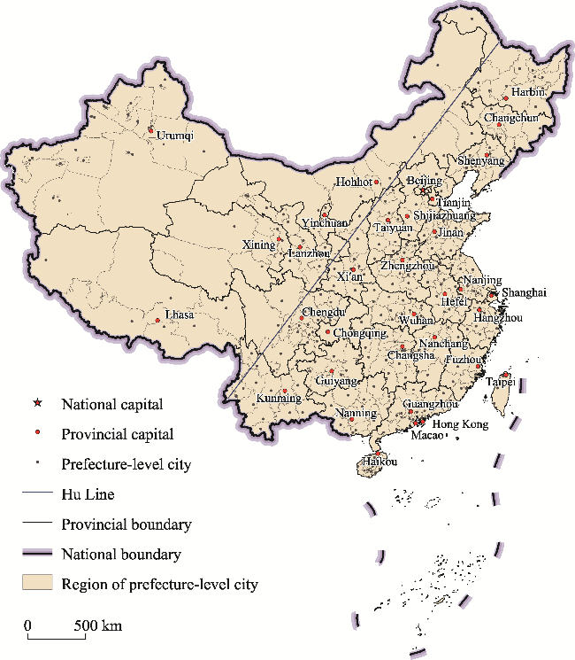
View original graphic|Download|PPT slide

Figure 1 Locations of major cities in China

(1) Baidu migration index (BMI)

BMI is publicly available through Baidu Map Huiyan spatio-temporal big data platform (https://huiyan.baidu.com/). Baidu, China’s largest search engine company, created an interactive map that displays people’s travel routes in China during the Spring Festival travel rush on 26 January 2014 (Wang et al., 2014). Since then, the dynamic state of population mobility in China in real-time, dynamically and intuitively during some specific periods (such as the Spring Festival travel rush, and the emergency period) can be observed. According to the report of QuestMobile, a leading mobile internet business intelligence services provider in China, Baidu has 118 enterprise applications, and the number of total users was 1.102 billion as of December 2023 (https://www.questmobile.com.cn/en, accessed on 25 April 2024). Given the widespread use of smart phones, if people allow Baidu application programs on various platforms to use the LBS of Baidu Map, the third-party users’ positioning information can be collected. The information is input into the Baidu cloud computing platform for statistical data processing to obtain real-time patterns of human migration. By summarizing and analyzing all the travel routes across the country, the residents’ flow trajectories are outlined using the city as the basic statistical unit. The flow process generally includes origin city and destination city nodes, as well as population flow intensity. This ensures that the data maintains horizontal comparability between cities. BMI is updated hourly for the travel routes in the last eight hours, displays every travel route people are traveling to and leaving from.

It has been proved that the BMI can accurately reflect the direction and intensity of population mobility between cities (Fang et al., 2020; Hu et al., 2020a). Generally, three types of population migration indexes, namely, daily inflow or outflow intensity index of each city, inflow or outflow proportion index to each city, and intra-city migration index, are provided. Given the research’s emphasis on intercity interactive network, it exclusively considers the first two indexes. The sample data of intensity index and proportion index are shown in Table 1 and Table 2 respectively. In Table 1, the inflow intensity index for Beijing is 6.3188. This value represents the proportion of the national population that moved to Beijing on January 1, 2020. Certainly, the migration intensity index alone does not fully capture the dynamics of population flow between cities. However, the corresponding migration proportion index provides convenience for us to explore intercity interaction. As shown in Table 2, on January 1, 2020, the proportion index of people moving from Beijing to Tianjin was 7.79%. This means that 7.79% of the total population moving out of Beijing were relocated to Tianjin.

Table 1 A sample of Baidu intensity index

Date	City	Type	Intensity index	Date	City	Type	Intensity index
2020/01/01	Beijing	in	6.3188	…	…	…	…
2020/01/01	Guangzhou	in	6.7779	2020/01/31	Dongguan	out	0.8933
2020/01/10	Hefei	out	3.7473

Note: “In” refers to inflow, and “out” refers to outflow.

Table 2 A sample of Baidu proportion index

Date	Origin city	Destination city	Type	Proportion index	Date	Origin city	Destination city	Type	Proportion index
2020/01/01	Beijing	Tianjin	in	7.79%	…	…	…	…	…
2020/01/01	Guangzhou	Nanjing	in	0.16%	2020/01/31	Dongguan	Hangzhou	out	0.18%
2020/01/10	Hefei	Lu’an	out	11.72%

Note: “In” refers to inflow, and “out” refers to outflow.

Accordingly, based on the two aforementioned indexes, the intercity travel scale index between cities can be determined using Eq. (1) (Lu et al., 2021a; Xiu et al., 2021):

(1) $R_{ij}^{d}\text{=}PI_{ij}^{d}\times SI_{j}^{d}$

where R_ij^dis the intercity travel scale index from city i to j on the specified date d. PI_ij^dis the proportion index from city i to j. SI_j^d is the intensity index from city i to j. Figure 2 has been drawn to facilitate a more intuitive understanding of this process.

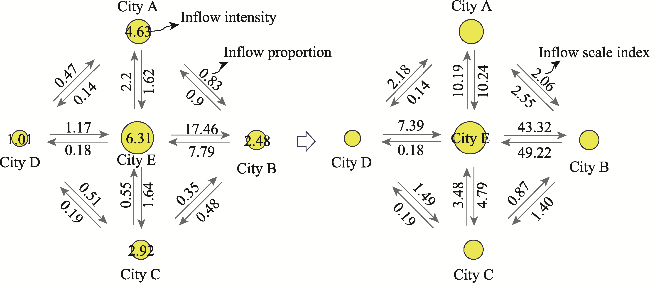
View original graphic|Download|PPT slide

Figure 2 Schematic of calculating intercity travel scale index based on intensity index and proportion index

(2) AutoNavi migration index (AMI)

AMI was derived from the AutoNavi transportation big data platform (https://trp.autonavi.com/migrate/page.do). AutoNavi Map (AMap) is one of the most popular map service providers in China. According to the report of QuestMobile, the number of monthly active users of AMap was more than 769.6 million as of December 2023. AutoNavi migration data is a national migration trajectory recorded by AMap and location data from third-party users based on LBS technology. Similarly to the BMI, AMI is a national population migration trajectory based on LBS, recorded through AMap and third-party user positioning data. It can also reflect the correlation features of intercity population mobility between cities (Zhou et al., 2020; Mu et al., 2022). Each AutoNavi migration record includes at least five fields, such as date, origin city, destination city, migration willingness index, and actual migration index. The sample data is shown in Table 3. The actual migration index records the completion of travel from one city to another using AMap’s navigation services. The migration willingness index reflects the behavior of searching for destinations and planning routes using AMap’s navigation services, representing people’s travel intentions rather than actual migration behavior. In this study, the actual migration index is employed to construct one of the intercity interactive networks.

Table 3 A sample of AMI data

Date	Origin city	Destination city	Migration willingness index	Actual migration index
2020/01/01	Beijing	Shanghai	0.8133	0.0247
2020/01/01	Chengdu	Chongqing	3.6081	1.0483
2020/01/02	Beijing	Shanghai	0.9786	0.0258
…	…	…	…	…
2020/01/31	Guangzhou	Shenzhen	5.4303	1.7781

(3) Mobile phone (MP) data

MP data is a type of anonymous and desensitized human activity data product (Wu et al., 2020; Zhang et al., 2020a), which is a variety of time-stamped and location-marked records produced by mobile phone during the use process, generally supplied by cellular communication operators. Whenever there is signal transmission between the mobile phone and the base station—such as powering on or off, making a call, sending a message, updating location, or switching base stations—the user’s location information is recorded and stored. MP data includes mobile phone signaling (MPS) data and Call Detail Record (CDR) data. As a new data source, the data has the characteristics of wide spatiotemporal coverage, large amount of data, timely update, and so forth. However, in contrast to the BMI and AMI, MP data is not publicly accessible. Fortunately, Lu et al. (2021b) have shared a dataset comprising 7810 origin-destination (OD) pairs detailing the intercity flow from Wuhan to various other cities in China, spanning from January 1 to 31, 2020. The data is further processed and aggregated population flow data based on China Unicom’s CDR data. Initially, it was aggregated and organized into daily intercity mobility matrices. Subsequently, the number of movements between cities was extrapolated to the whole network based on a variety of user demographics and operator coverage differences. The sample data are shown in Table 4. Fields such as date, city and outflow scale were provided. For instance, the population scale from Wuhan to Beijing was 4927 on January 1, 2020. The data has been compared and validated with demographic data and BMI data, demonstrating high accuracy with all R-squared values exceeding 0.9 (Lu et al., 2021b). It facilitated the conduct of this research.

Table 4 A sample of mobile phone data from Wuhan to other cities in China

Date	City	City code	Province	Latitude	Longitude	Outflow scale
2020/01/01	Anqing	340,800	Anhui	30.543494	117.063754	1067
2020/01/02	Beijing	110,000	Beijing	39.904030	116.407526	4927
2020/01/02	Chongqing	500,000	Chongqing	29.563009	106.551556	2525
…	…	…	…	…	…	…
2020/01/31	Huanggang	421,100	Hubei	30.453905	114.872316	11,935

Table 5 presents the characteristics of the intercity population migration data from Baidu, AutoNavi and MP. To maintain comparability, the data collection period for both Baidu and AutoNavi has been similarly confined to January 1 to 31, 2020. Obviously, all three types of data feature a daily time resolution, enabling them to dynamically and visually express the population migration trajectories in real-time. Nonetheless, significant variations exist in their sources of acquisition, radiation areas, and OD pairs. Contrastingly, AMI data encompasses a more thorough understanding of urban nodes, covering 366 city units, whereas BMI data incorporates only 327 city units. It predominantly omits county-level cities directly governed by the provincial authorities in Hubei, Hainan, Xinjiang, and Xizang. Furthermore, the intercity OD pairs over the 31-day study period also reveal that migration trajectories from AutoNavi surpass those of Baidu. Finally, it should be noted that the MP data represents extrapolated data of the mobile population based on China Unicom’s records, serving only as a relative reference, rather than an absolute benchmark.

Table 5 Characteristics of Baidu, AutoNavi and mobile phone intercity population migration data

Variable	BMI	AMI	MP
Source	Baidu LBS	AMap LBS	China Unicom
Time-period	2020.01.01-2020.01.31	2020.01.01-2020.01.31	2020.01.01-2020.01.31
Spatial scope	327 urban units	366 urban units	339 urban units
National intercity OD pairs	984,905	1,765,150	—
Intercity OD pairs from Wuhan	8273	8990	7810

3 Research framework and methods

3.1 Research framework

A novel research framework (Figure 3) is proposed for uncovering the differences in spatial structure of intercity interactive networks at multiple levels represented by multi-source migration big data. Initially, multi-source migration big data, namely, BMI, AMI, and MP, during the same time-period are collected. After a series of data cleaning, the intercity interactive networks at different spatial scales (national flow and Wuhan outflow) are constructed respectively. Then, their overall characteristics and correlations are revealed using complex network analysis. Furthermore, the spatial structures of intercity interactive networks, predicated on population migration data from Baidu and AutoNavi, are extracted at multiple levels using the multi-hierarchical method proposed by Zhou et al. (2024a). Accordingly, the similarities in the network spatial structure at multiple levels are further quantified and analyzed from three critical perspectives: node location, node size, and local structure.

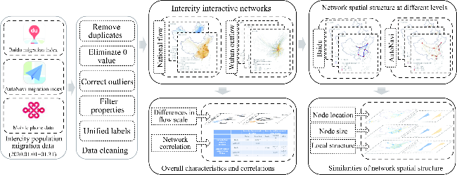
View original graphic|Download|PPT slide

Figure 3 Research framework for revealing the differences in spatial structure of intercity interactive networks

3.2 Methods

3.2.1 Complex network analysis

(1) Construction of intercity interactive network

Wei et al. (2018) pointed out that the intercity interactive network exemplifies a typical directed and weighted geographical network, characterized by fixed nodes and a fundamental attribute of uneven distribution in the intercity population flows. The construction of the intercity interactive network in this study hinges on the utilization of an intercity OD matrix. The daily intercity OD matrix, derived from the processed big data on intercity population migration, is expressed as demonstrated in Eq. (2) (Pan and Lai, 2019):

(2) $\begin{align} & \begin{matrix} \begin{matrix} {} & \begin{matrix} \begin{matrix} {} & {} \\ \end{matrix} \\ \end{matrix} \\ \end{matrix} & {{j}_{1}} & {{j}_{2}} &. &. &. & {{j}_{(n-1)}}{{j}_{n}} & {} & {} \\ \end{matrix} \\ & L(t)=\begin{matrix} {{i}_{1}} \\ {{i}_{2}} \\. \\. \\. \\ {{i}_{(n-1)}} \\ {{i}_{n}} \\\end{matrix}\left[ \begin{matrix} 0 & {{L}_{12}} &. &. &. & {{L}_{1(n-1)}} & {{L}_{1n}} \\ {{L}_{21}} & 0 &. &. &. & {{L}_{2(n-1)}} & {{L}_{2n}} \\. &. &. &. &. &. &. \\. &. &. &. &. &. &. \\. &. &. &. &. &. &. \\ {{L}_{1(n-1)}} & {{L}_{2(n-1)}} &. &. &. & 0 & {{L}_{n(n-1)}} \\ {{L}_{1n}} & {{L}_{2n}} &. &. &. & {{L}_{n(n-1)}} & 0 \\ \end{matrix} \right] \\ \end{align}$

where L(t) represents the intercity interactive OD matrix for a designated date t. L_ij is the intercity migration scale index from city i to city j. Accordingly, the average intercity interactive OD matrix in the corresponding time-period is calculated, thereby constructing the intercity interactive network. The equation is as follows:

(3) $L=\frac{1}{m}\sum\limits_{t=1}^{m}{L(t)}$

where L indicates the average intercity interactive OD matrix. m is the total days during the research period.

(2) Intercity interactive scale

The daily intercity interactive scale for city i is the total volume of intercity trips for which city i serves as either the origin or the destination on the specified date t. The equation is as follows:

(4) $I{{S}_{it}}=IS_{it}^{in}+IS_{it}^{out}$

where IS_it is the intercity interactive scale of city i on the specified date t. $IS_{it}^{in}$ is the inflow scale of intercity interactive scale of city i on the specified date t, and $IS_{it}^{out}$ it is the outflow scale of intercity interactive scale of city i on the specified date t.

(3) Quadratic assignment procedure (QAP) correlation analysis

The QAP focuses on determining the degree of similarity or correlation between two or more matrices. The method employs matrix data substitution to evaluate the similarity of corresponding elements in two N×N matrices, thereby deriving a correlation coefficient for each matrix pair. Concurrently, a nonparametric test is applied to these coefficients to assess their statistical significance (Krackardt, 1987). The absence of a requirement for variable independence confers a distinct advantage on this approach for representing correlations within relational data. This method is extensively employed to investigate network relevance, determine influential factors, and analyze formation mechanisms (Xu and Cheng, 2016). Undoubtedly, before performing the QAP analysis on the intercity networks, we normalized all scales of intercity interactions using Eq. (5) (He et al., 2023).

(5) ${{X}_{\text{norm}}}=\frac{X-{{X}_{\min }}}{{{X}_{\max }}-{{X}_{\min }}}$

where X_normstands for the normalized value, X for the original data, X_min and X_max for the minimum and maximum values of the original data, respectively.

3.2.2 Network spatial structure extraction

The methodology employed herein for extracting the multi-level spatial structure of intercity interactive networks refers to the model developed by Zhou et al. (2024a). The specific steps for implementation are as follows: (1) Construct the intercity interactive network utilizing data on intercity population migration; (2) Determine the spatial proximity network by assessing whether nodes share spatial boundaries; (3) Build the maximum spanning tree (MST) focusing on edges that are adjacent and demonstrate strong interactions; (4) Create the initial population based on MST, and then conduct iteration and update of population through a genetic algorithm, and (5) Extract the optimal solution modularity-based from the iterations to delineate the final network spatial structure. The more detailed process of extracting network spatial structure can be referred to the researches by Zhou et al. (2024a) and Xu et al. (2023), which will not be reiterated herein.

3.2.3 Measuring similarity in network structures

In this study, we conduct a comprehensive measure of network structure similarities from three distinct perspectives (Node location, node size, and local structure), as illustrated in Figure 4, with each measure grounded in their spatial relationships.

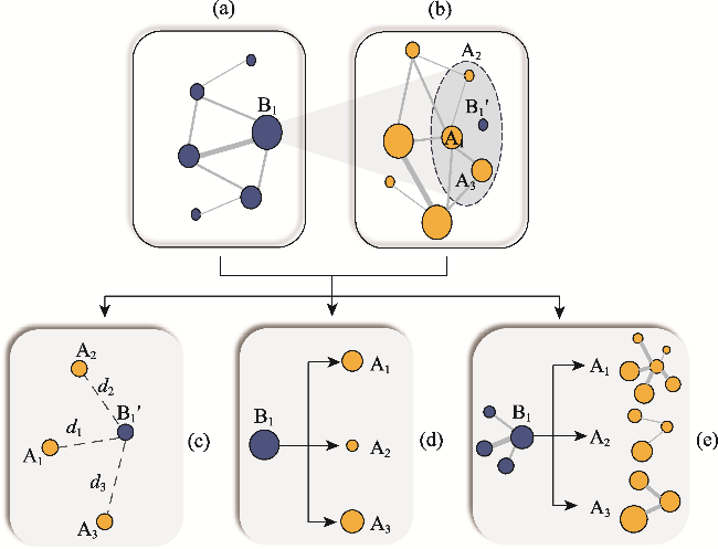
View original graphic|Download|PPT slide

Figure 4 Schematic of location projection and similarity measuring in network structures (a. Baidu network; b. AutoNavi network; c. Euclidean distance based on the location of nodes; d. Nodes and their size; e. Local network structure)

(1) Node location similarity

To measure the node location similarity between two types of intercity networks, this study first identifies and matches corresponding nodes in one network to those in another based on their spatial location. Subsequently, the location similarity is quantified using a distance method. Specifically, the process involves two steps: (1) Identifying network nodes with analogous spatial location (Figures 4a and 4b). Initially, nodes from two networks are spatially mapped to one another. Following this mapping, a predetermined number of target nodes, which share similar spatial positions, are identified using the preset k-nearest neighbor value. (2) Measuring the average location similarity of nodes. Firstly, the Euclidean distances between each mapping node and its corresponding target nodes using their spatial coordinates are determined (Figure 4c). The average location similarity of nodes is then calculated by incorporating the radial basis kernel function, which is formulated as follows (Xu et al., 2023):

(6) ${{S}_{L}}\text{=}\frac{1}{k}\sum\limits_{i=1}^{k}{{{e}^{-\frac{{{\left\| x-{{c}_{i}} \right\|}^{2}}}{2{{\sigma }^{2}}}}}}$

where S_Ldenotes the node location similarity, with values ranging from 0 to 1. Higher values correspond to greater similarity of node location. k represents a predefined parameter in the k-nearest neighbor algorithm. ||x-c_i||²stands for the Euclidean distance between the mapping node and the target nodes in the two types of networks. σ is a free parameter that controls the range of action of the kernel function.

(2) Node size similarity

The process for assessing node size similarity closely mirrors that used for evaluating location similarity. The analytical approach commences with two types of networks, aiming to quantify the similarity in size between the mapping node and the target nodes (Figure 4d). Node size is defined as the cumulative intensity of interaction flows among the original nodes within a group. Specifically, the process involves three steps: (1) determining the nodes sets with adjacent location according to their spatial mapping relationships (Figures 4a and 4b); (2) calculating the size similarities between a node and each node within its corresponding node set; (3) obtaining the average node size similarity. The equation is as follows (Xu et al., 2023):

(7) ${{S}_{S}}\text{=1}-\frac{1}{k}\sum\limits_{i=1}^{k}{\frac{\left| Siz{{e}_{{{B}_{1}}}}-Siz{{e}_{{{A}_{i}}}} \right|}{\max (Siz{{e}_{{{B}_{1}}}},Siz{{e}_{{{A}_{i}}}})}}$

where S_S denotes the node size similarity, with values ranging from 0 to 1. Higher values correspond to greater similarity of node size. $Siz{{e}_{{{B}_{1}}}}$ and $Siz{{e}_{{{A}_{i}}}}$ represent the size of node B₁ and node A_i, respectively.

(3) Local structure similarity

Xu et al. (2023) defined the fundamental unit of network structure as a “node-edge-node” and quantified structure similarity from the perspective of network association. This framework has also been employed in this study. Specifically, (1) the network structure units comprising nodes with proximate spatial location are identified (Figure 4e). (2) The node degree (ND, the number of all neighbor nodes owned by a node), node weight (NW, the sum of the sizes of all neighbor nodes owned by a node), and edge weight (EW, the sum of the sizes of the edges connecting a node and all its neighbors) have been chosen as measurement indicators. Consequently, a three-dimensional vector representing the node’s structure characteristics is constructed, exemplified by a ${{\overset{\scriptscriptstyle\rightharpoonup}{A}}_{1}}$ = (ND₁, NW₁, EW₁). (3) Calculating the covariance matrix C for the three-dimensional structure vectors of k+1 structure units using Eq. (8) (Xu et al., 2023):

(8) $C=\left( \begin{align} & cov(ND,ND)cov(ND,NW)cov(ND,EW) \\ & cov(NW,ND)cov(NW,NW)cov(NW,EW) \\ & cov(EW,ND)cov(EW,NW)cov(EW,EW) \\ \end{align} \right)$

where cov(X, Y) stands for the covariance of X, Y, denoted as follows:

(9) $cov(X,Y)\text{=}\frac{\sum\limits_{n=1}^{n}{({{X}_{i}}-\overline{X})({{Y}_{i}}-\overline{Y})}}{n-1}$

where n represents the number of structure vectors. $\overline{X}$ and $\overline{Y}$ are the mean value of two dimensions, respectively.

Finally, the local structure similarity is quantified using the Mahalanobis distance. The equation is as follows (Xu et al., 2023):

(10) ${{S}_{St}}\text{=}\frac{1}{k}\sum\limits_{i=1}^{k}{\sqrt{{{({{{\overset{\scriptscriptstyle\rightharpoonup}{B}}}_{1}}-{{{\overset{\scriptscriptstyle\rightharpoonup}{A}}}_{i}})}^{T}}{{C}^{-1}}({{{\overset{\scriptscriptstyle\rightharpoonup}{B}}}_{1}}-{{{\overset{\scriptscriptstyle\rightharpoonup}{A}}}_{i}})}}$

where S_St denotes the local structure similarity. Smaller values correspond to greater similarity of local network structure. C^–1 is the inverse matrix of the covariance matrix C. ${{\overset{\scriptscriptstyle\rightharpoonup}{B}}_{1}}$ and ${{\overset{\scriptscriptstyle\rightharpoonup}{A}}_{i}}$ are the structure vectors of node B₁and V₁, respectively.

4 Results

4.1 Overall characteristic and correlation of intercity interactive networks

The spatial distribution of intercity interactive networks in China represented by Baidu and AutoNavi migration data is shown in Figure 5. Generally, the intercity interactive networks of Baidu and AutoNavi exhibit a higher concentration to the southeast of Hu Line (also known as Heihe-Tengchong Line, the dividing line of population density in China) and are markedly less dense to the northwest of the line. Figure 5a illustrates Baidu intercity interactive network, encompassing 327 urban nodes and 13,692 connections. Figure 5b showcases the AutoNavi intercity interactive network, which includes 366 urban nodes and 24,660 connections. The latter network exhibits a broader scale with more frequent intercity interactions compared to the former, possessing a network density of 0.185, which is 1.45 times higher. Nevertheless, the former network displays a pronounced cross-regional characteristic, with stronger connections to the west of the Hu Line. Additionally, it demonstrates a more potent radiation effect of the core city on its hinterland region. In any case, the structure differences between the two types of networks are beginning to emerge.

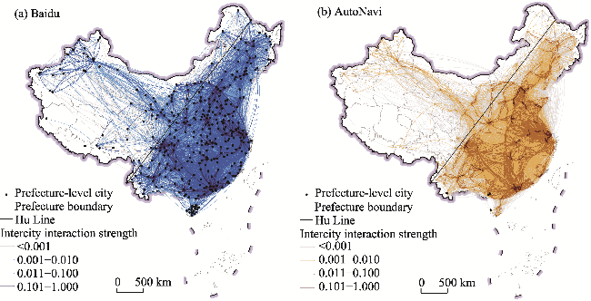
View original graphic|Download|PPT slide

Figure 5 Spatial pattern of intercity interactive networks in China (a. Baidu; b. AutoNavi)

Further analysis is warranted to elucidate the allocation and cumulative rates of intercity interactive flows across varying distances. It can be seen from Figure 6 that the intercity interactions as indicated by Baidu and AutoNavi all exhibit a distance attenuation effect, where the scale of interaction diminishes progressively with an increase in distance. While Baidu and AutoNavi intercity interactive networks display comparable trends in distance distribution, the data suggests that the distance attenuation effect is relatively more pronounced in migrations recorded by the latter. Specifically, within the 0-200 km range, the proportion of AutoNavi intercity interactions is 61.20%, surpassing Baidu’s equivalent at 51.24%. Beyond this threshold, the rate of decrease in interactive scale with increasing distance was more pronounced for AutoNavi than for Baidu. Moreover, the AutoNavi migration activities are mostly concentrated within the 0-1400 km distance range, representing 98.87% of its total flows, whereas Baidu migration activities are distributed within a slightly broader range of 0-1600 km, representing 98.01% of its flows.

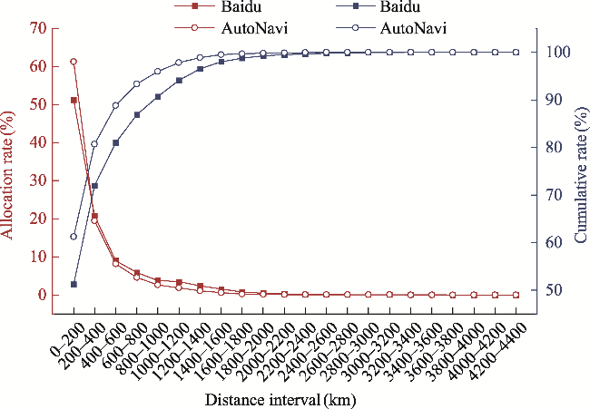
View original graphic|Download|PPT slide

Figure 6 Distribution of distance in intercity interactive scale in China

The intercity flow scale for each urban node within the Baidu and AutoNavi intercity interactive networks has been calculated. Their results are presented in Figure 7. It is evident that significant disparities exist in terms of both the flow scale and rank of urban nodes. On the one hand, the total scale of intercity flow as indicated by Baidu migration slightly surpasses that derived from AutoNavi, reaching peak figures of 11.12 and 6.20, respectively. On the other hand, regardless of whether Baidu or AutoNavi intercity interaction, the top 20 cities predominantly are the core cities within China’s five major urban agglomerations. However, it is evident that the core cities of four urban agglomerations are competing for dominance in Baidu intercity network, exhibiting a pronounced “rich-club” phenomenon (Wei et al., 2018). Notable examples include Beijing, Chengdu, Chongqing, Shanghai, Guangzhou, Shenzhen, and others. While in AutoNavi intercity network, there is a significant hierarchical distribution feature, followed by the core cities of the Pearl River Delta, Yangtze River Delta, Chengdu-Chongqing, Beijing-Tianjin-Hebei, and the middle reaches of Yangtze River urban agglomerations.

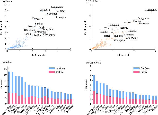
View original graphic|Download|PPT slide

Figure 7 The intercity interaction strength of urban nodes (a-b. Distribution of urban outflow and inflow scales; c-d. Top 20 cities of total scale)

To verify data accuracy, the Wuhan’s intercity outflow subnetworks from both Baidu and AutoNavi migration were extracted and then compared with the Wuhan’s intercity outflow network derived from MP. The findings suggest that in comparison with the Wuhan’s intercity outflow network from MP, the AutoNavi subnetwork more closely approximates in both scale and range of interaction. The number of intercity outflow routes is ranked as follows: AutoNavi with 344 lines, MP with 338 lines, and Baidu with 326 lines. Regarding the average interactive distance, it is ranked as follows: MP with 1068 km, AutoNavi with 1054 km, and Baidu with 1015 km. In addition, the hierarchical structure of AutoNavi intercity interactive subnetwork demonstrates greater consistency, whereas Baidu intercity interactive subnetwork exhibits significant spatial heterogeneity. Moreover, as presented in Table 6, the sequence of routes in AutoNavi intercity interactive subnetwork more closely mirrors that of the MP.

Table 6 Top 20 routes of Wuhan’s intercity outflow network from Baidu, AutoNavi and MP migration data

Rank	Baidu	AutoNavi	MP
1	Wuhan→Xiaogan	Wuhan→Xiaogan	Wuhan→Xiaogan
2	Wuhan→Huanggang	Wuhan→Huanggang	Wuhan→Ezhou
3	Wuhan→Jingzhou	Wuhan→Ezhou	Wuhan→Huanggang
4	Wuhan→Xianning	Wuhan→Xianning	Wuhan→Xianning
5	Wuhan→Ezhou	Wuhan→Jingzhou	Wuhan→Jingzhou
6	Wuhan→Xiangyang	Wuhan→Huangshi	Wuhan→Huangshi
7	Wuhan→Huangshi	Wuhan→Xiantao	Wuhan→Xiantao
8	Wuhan→Jingmen	Wuhan→Jingmen	Wuhan→Jingmen
9	Wuhan→Suizhou	Wuhan→Suizhou	Wuhan→Xiangyang
10	Wuhan→Yichang	Wuhan→Xiangyang	Wuhan→Suizhou
11	Wuhan→Enshi	Wuhan→Tianmen	Wuhan→Tianmen
12	Wuhan→Shiyan	Wuhan→Xinyang	Wuhan→Yichang
13	Wuhan→Chongqing	Wuhan→Yichang	Wuhan→Xinyang
14	Wuhan→Beijing	Wuhan→Chongqing	Wuhan→Enshi
15	Wuhan→Xinyang	Wuhan→Changsha	Wuhan→Shiyan
16	Wuhan→Changsha	Wuhan→Zhumadian	Wuhan→Changsha
17	Wuhan→Shanghai	Wuhan→Qianjiang	Wuhan→Qianjiang
18	Wuhan→Zhengzhou	Wuhan→Enshi	Wuhan→Zhumadian
19	Wuhan→Guangzhou	Wuhan→Shiyan	Wuhan→Zhengzhou
20	Wuhan→Shenzhen	Wuhan→Yueyang	Wuhan→Beijing

The aforementioned indicators suggest a higher degree of similarity between the AutoNavi and MP intercity interactive networks. This hypothesis is corroborated by network correlation analysis employing QAP. Utilizing the UCINET social network analysis tool, the correlations between China’s (Baidu, AutoNavi) and Wuhan’s outflow (Baidu, AutoNavi, MP) intercity interactive networks were analyzed. The correlation coefficients are presented in Table 7. There is significant correlation between them. The correlation coefficients are all above 0.87, and the P-value is less than 0.01, implying a statistical significance. At the overall level, the Baidu and AutoNavi intercity networks exhibit a high degree of correlation, with a correlation coefficient of 0.874. At the local scale, both Baidu and AutoNavi intercity networks demonstrate a strong correlation with the MP intercity network, with correlation coefficients exceeding 0.90. Notably, the correlation between the AutoNavi and MP network is markedly stronger, evidenced by a correlation coefficient of 0.954.

Table 7 QAP correlation analysis of intercity interactive networks

		China’s intercity interactive network		Wuhan’s intercity outflow network
		Baidu	AutoNavi	Baidu	AutoNavi	MP
China’s intercity interactive network	Baidu	1.000	0.874**	-	-	-
China’s intercity interactive network	AutoNavi		1.000	-	-	-
Wuhan’s intercity outflow network	Baidu	-	-	1.000	0.977**	0.908**
	AutoNavi	-	-		1.000	0.954**
	MP	-	-			1.000

Note: ** indicates a significant correlation at 1% level.

4.2 Spatial structure of intercity interactive networks at different levels

Zhou et al. (2024a) extracted network spatial structure by aggregating adjacent nodes with strong interactions and dissociating those with weak connections, thereby capturing the inherent spatial patterns and relationships within a network. This approach is grounded in two fundamental geographical assumptions: spatial autocorrelation and spatial heterogeneity. It effectively realizes the extraction of network spatial structure from large-scale OD network data. Different from the methodology they proposed, the final position of nodes is determined by calculating the center of gravity of the sub-nodes within a group in this study. Nodes with greater interaction strength exert more influence and, consequently, are positioned nearer to the center of a group. Figure 8 draws the spatial pattern of China’s intercity interactive network, comprising 10, 20, and 30 nodes, as constructed using Baidu and AutoNavi migration. The total strength of nodes denotes the aggregate of relative intercity interaction strength between the sub-nodes within a group. Interaction strength is defined as the cumulative intercity flow strength between sub-nodes affiliated with two distinct groups, reflecting the interactive extent between nodes.

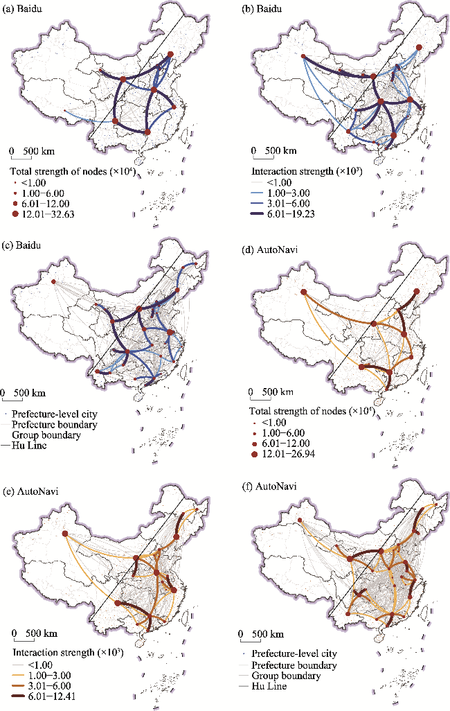
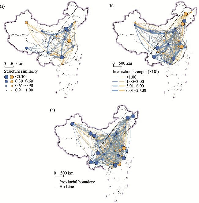
View original graphic|Download|PPT slide

Figure 8 Spatial structure of intercity interactive network in China at different levels (a-c. Baidu networks with 10, 20, 30 nodes; d-f. AutoNavi networks with 10, 20, 30 nodes)

Generally speaking, in the Baidu and AutoNavi intercity interactive networks at different levels, a preponderance of the nodes is situated southeast of the Hu Line. As the node threshold increases from 10 to 30, there is a discernible migration of the center of gravity of nodes in the networks towards regions with dense populations, robust economic development, and well-established transportation systems, concurrently presenting to a more distinctly node hierarchy. Meanwhile, their distribution is more homogeneous across the spatial. Moreover, while the intercity interactive connections remain predominantly situated to the east of the Hu Line, an increased node threshold has led to the emergence of new connections mainly in the central and northeastern regions of China. Considering the aforementioned points, while spatial structures of the two networks share numerous commonalities, the differences between them are significant and must not be overlooked.

In the Baidu intercity networks (as shown in Figures 8a-8c), strong interaction connections (interaction strength > 6.01 × 10³) are considerably more than that in the AutoNavi intercity networks (Figures 8d-8f). The former exhibits strong cross-regional interactions at all levels, while the latter network’s strong interactions are primarily concentrated between neighboring nodes. This indicates that the Baidu intercity interactive network shows strong advantages in overcoming the spatial friction effect. Furthermore, within the Baidu networks, a lower threshold corresponds to a more concentrated spatial distribution of network nodes. Conversely, the AutoNavi networks exhibit a more homogeneous spatial distribution, with the positioning of high-level nodes (the total strength of nodes > 12.01 × 10⁴) remaining more consistent.

The number of original sub-nodes included in the final node is counted. These are presented in descending order in Figure 9. Combined with Figure 8, it becomes evident that there is a significant variance in the geographic and spatial combination of cities corresponding to nodes in Baidu and AutoNavi networks. The former demonstrates a more pronounced discrepancy in the number of sub-nodes between leading and trailing nodes, whereas the latter exhibits greater uniformity. In other words, the Baidu intercity interactive network exhibits more significant spatial heterogeneity. In terms of spatial distribution, a discernible spatial dislocation is present at the node group boundaries of each level of these networks, particularly pronounced in networks with smaller thresholds. Such misalignment establishes a basis for analyzing network structure similarities from a spatial standpoint. This phenomenon lays a foundation for analyzing the similarity of network structures from a spatial perspective.

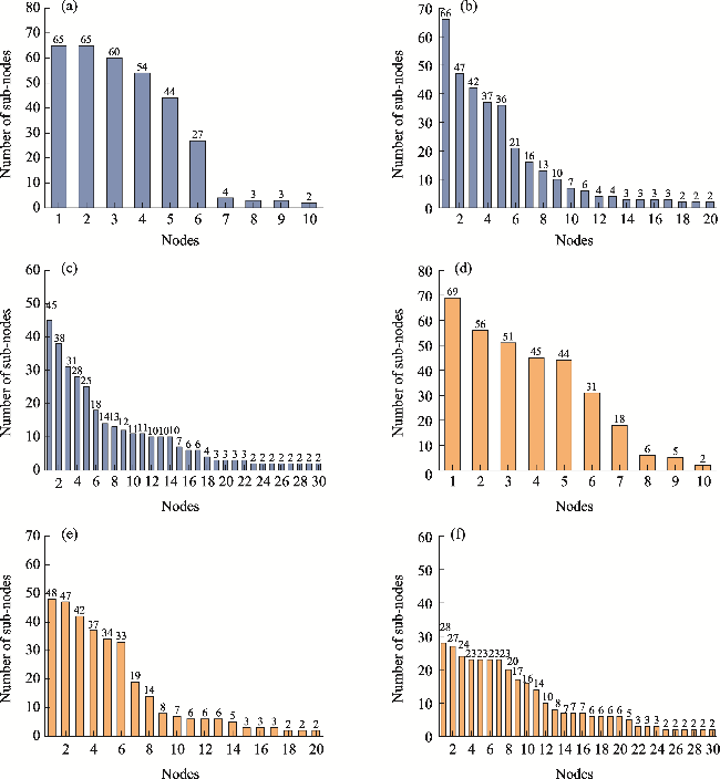
View original graphic|Download|PPT slide

Figure 9 Statistics of sub-nodes for each final node in the intercity interactive networks at different levels (a-c. Baidu; d-f. AutoNavi)

4.3 Spatial structure similarities of intercity interactive networks

The preceding analysis reveals that, within the network spatial structures at each level derived from the Baidu and AutoNavi intercity interactive networks, there is a noticeable dislocation in the spatial positioning of nodes. This misalignment underscores a characteristic difference in network structure. To deepen the understanding of the spatial structure similarity in intercity interactive networks, this study embraces a relevance analytical perspective that is conducted across three dimensions, namely, node location, node size, and local structure, respectively. The traditional methods of network comparison are evidently inadequate for current complexities. Consequently, this study employs the “one-to-many” spatial mapping relationship introduced by Xu et al. (2023) as a framework to assess the similarity of spatial and non-spatial attributes in the Baidu and AutoNavi intercity interactive networks.

4.3.1 Node location similarity

Figure 10 presents the node location similarities for the two types of intercity interactive networks as calculated according to Eq. (6). The Baidu and AutoNavi networks are distinguished by blue and yellow respectively, a convention that is consistently applied in subsequent similar visualizations. Their spatial distribution reveals variances in the location similarity of network structures across different levels. However, generally, as the node threshold rises, nodes exhibiting higher location similarity (> 0.65) progressively expand toward the northwest and northeast. These nodes are predominantly concentrated in the Beijing-Tianjin-Hebei, Yangtze River Delta, Pearl River Delta, and Southwest China. This pattern indicates that the location similarity between Baidu and AutoNavi networks is consistent in spatial distribution.

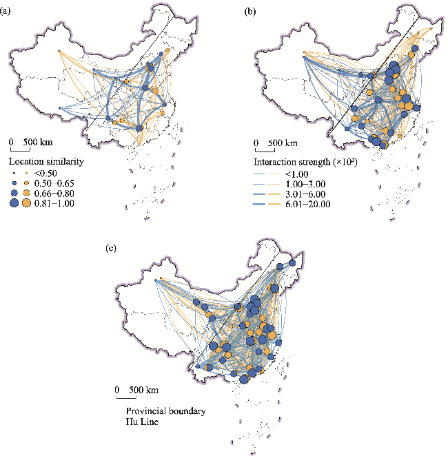
View original graphic|Download|PPT slide

Figure 10 Node location similarity (nodes and links corresponding to Baidu and AutoNavi network are blue and yellow, respectively) (a. 10 nodes; b. 20 nodes; c. 30 nodes)

Specifically, in the networks characterized by a node threshold of 10 (Figure 10a), the Baidu network exhibits greater node location similarity to the AutoNavi network. It presents a larger number of nodes with higher location similarity and fewer nodes with moderate low location similarity (0.50-0.65). In the networks characterized by a node threshold of 20 (Figure 10b), Baidu and AutoNavi networks display a comparable number of nodes with location similarity across all levels. The Baidu network has only one additional node compared to the latter in the level with moderate high location similarity (0.66-0.80) and one fewer node in the level of low location similarity (< 0.50). Moreover, the spatial distribution of nodes between the two networks also exhibits a high degree of similarity. In the networks characterized by a node threshold of 30, as depicted in Figure 10c, the number of nodes with moderate high location similarity between Baidu and AutoNavi networks is not only large but also equal. However, the former network has more nodes at the level of high location similarity (0.81-1.00). Spatially, it is mainly reflected in regions such as Chengdu- Chongqing and Northeast China. These findings indicate that both types of network have a high degree of node location similarity. However, in the latter network, nodes with higher location similarity demonstrate more pronounced characteristics of spatial concentration. These findings indicate that the two types of intercity interactive networks exhibit a high degree of similarity in node locations. Additionally, nodes with higher location similarity in the AutoNavi network display more concentrated spatial distribution characteristics.

The violin plots of node location similarity between Baidu and AutoNavi networks (Figure 11) are depicted to further analyze the details of their distribution characteristics. It can be seen that as the node threshold increases, there is a corresponding rise in the average node location similarity. In the two types of networks comprising 10, 20, and 30 nodes, the average location similarity is approximately 0.57, 0.71, and 0.77, respectively. Furthermore, at a node threshold of 20, the distribution of node location similarity across the two types of networks exhibits a more consistent trend, which may provide an empirical foundation for subsequent related research.

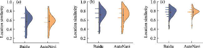
View original graphic|Download|PPT slide

Figure 11 Violin plot of node location similarity (a. 10 nodes; b. 20 nodes; c. 30 nodes)

4.3.2 Node size similarity

Figure 12 shows the node size similarities for the two types of intercity interactive networks as measured according to Eq. (7). Overall, as the node threshold rises, there is a notable increase in the nodes exhibiting higher size similarity (> 0.45) within both types of networks, especially from the perspective of the Baidu network. This suggests that the Baidu network has higher similarity with the AutoNavi network in terms of node size. In terms of spatial distribution, the former network exhibits a trend toward increased agglomeration in the Beijing-Tianjin-Hebei region, whereas it presents an increasingly dispersed distribution pattern in other regions. The latter network is primarily concentrated in the Yangtze River Delta, the Central China Plains, and Southwest China. These patterns indicate that the node size similarities of the two types of networks demonstrate significant spatial differentiation characteristics.

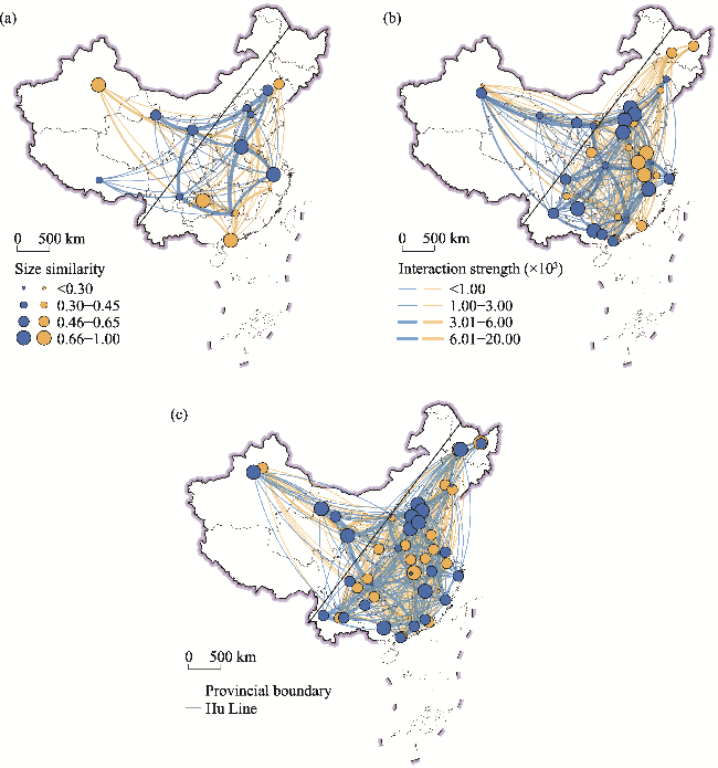
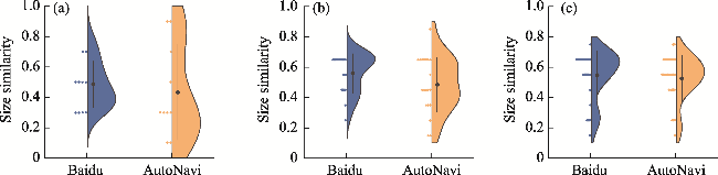
View original graphic|Download|PPT slide

Figure 12 Node size similarity (nodes and links corresponding to Baidu and AutoNavi network are blue and yellow, respectively) (a. 10 nodes; b. 20 nodes; c. 30 nodes)

In the networks delineated by a node threshold of 10 (Figure 12a), the node size similarity from the Baidu network perspective is more significant than that in the AutoNavi network perspective. Specifically, the quantity of nodes exhibiting moderate high size similarity in the Baidu network is 5, which exceeds that of the AutoNavi network. Meanwhile, there is only one node with low similarity (< 0.30) in the former, while the letter contains 5 nodes. Correspondently, the spatial differentiation between the two types of networks is pronounced. In the networks delineated by a node threshold of 20 (Figure 12b), from the perspective of Baidu network, the number of nodes with high size similarity (0.66-1.00) is more, with a number of 7, which is spatially concentrated prominently in the regions of Beijing-Tianjin- Hebei and Southwest China. From the perspective of AutoNavi network, the nodes with high size similarity are mostly concentrated in East China and North China, while the nodes with moderate low size similarity (0.3-0.45) are not only larger in number, but also principally distributed to the east of the Hu Line, demonstrating a relatively dispersed spatial distribution pattern. In the networks delineated by a node threshold of 30 (Figure 12c), the analysis conducted through the Baidu network highlights that there is a significant presence of nodes with high size similarity, totaling 11, which exhibit a concentrated distribution in the Beijing-Tianjin-Hebei region, yet display a dispersed pattern elsewhere. However, analysis through the AutoNavi network identifies 20 nodes with moderate high size similarity, which is more than the Baidu perspective, and they are characterized by a notably more compact spatial distribution.

The violin plots of node size similarity between Baidu and AutoNavi networks are dawned in Figure 13. As can be seen from them, the average size similarity of nodes is consistently higher when analyzed from the Baidu network perspective compared to the AutoNavi network. However, it is obvious that the disparity between the two is showing a trend of gradual diminution. Further analysis reveals that as the node threshold rises, the distribution of node size similarity between the two types of networks becomes more consistent. That is, maintaining the node threshold at 30 leads to a higher similarity in node size across both types of networks, with most values falling between 0.5 and 0.7.

View original graphic|Download|PPT slide

Figure 13 Violin plot of node size similarity (a. 10 nodes; b. 20 nodes; c. 30 nodes)

4.3.3 Local structure similarity

The results of the local structure similarity for the two types of intercity interactive networks measured by combining node degree, node weight, and edge weight are displayed in Figure 14. As a whole, in different levels of the Baidu and AutoNavi networks, there are great differences in the local structure similarity from the perspective of dual networks. The majority of local structure units exhibit lower similarity (> 0.60). The quantity of local structural units exhibiting higher similarity (≤ 0.60) is not only limited but also demonstrates a notable distinct in their spatial distribution.

View original graphic|Download|PPT slide

Figure 14 Local structure similarity (nodes and links corresponding to Baidu and AutoNavi network are blue and yellow, respectively) (a. 10 nodes; b. 20 nodes; c 30 nodes)

Detailly, in the networks with a node threshold of 10 (Figure 14a), from the perspective of dual networks, there are only two structure units with high structure similarity (< 0.3). Furthermore, this significant correlation is observed exclusively in the Beijing-Tianjin-Hebei region. The local structure units with moderate high similarity (0.30-0.60) had large spatial distribution differences. In the networks delineated by a node threshold of 20 (Figure 14b), more matching structure units have been identified in Northeast China. In addition, the local structure units exhibiting high similarity from the perspective of the Baidu and AutoNavi networks are predominantly distributed in Southwest and Southeast China, respectively. In the networks characterized by a node threshold of 30 (Figure 14c), the perspective of the Baidu network reveals numerous local structural units with high structure similarity in the southeast coast, southwest, northeast, and northwest regions. However, it is noteworthy that only the southeast coast exhibits a high degree of matching with the AutoNavi network. This indicates that the intercity “circle of friends” within this region exhibit greater convergence or consistency across the two network types, in contrast to those in other regions.

The violin plot (Figure 15) descripting local structure similarity between the dual networks indicates that the average similarity of local structure units, as observed from the Baidu network perspective, is typically lower in comparison to those observed from the AutoNavi network perspective. In other words, the perspective of Baidu network exhibits larger similarity with the AutoNavi network. However, this difference between the two is minimized when the node threshold is set at 20. Meanwhile, their distribution trends align more coincidently, showing the characteristics of fewer high similarity and more low similarity. This suggests that at a node threshold of 20, the local structure units within the two types of networks exhibit stronger similarities. However, there is a significant difference in their local interaction patterns.

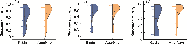
View original graphic|Download|PPT slide

Figure 15 Violin plot of local structure similarity (a. 10 nodes; b. 20 nodes; c. 30 nodes)

5 Discussion

5.1 Significances and contributions

Leveraging big data technology, the continuous emergence of spatiotemporal big data, which encapsulates the spatiotemporal distribution and real-time flow characteristics of the population, has paved the way for numerous research opportunities. However, multimodal social perception data exhibit varying capabilities in delineating urban spatial patterns and regional spatial structures. In this study, a comprehensive and in-depth comparison and explanation of the intercity interactive networks and their spatial structures at multiple levels were conducted, with a particular emphasis on the perspective of population flow. By constructing Baidu, AutoNavi, and MP intercity interactive networks for the same period, the similarities and correlations among them were explored. This research aims to provide empirical evidence for discerning the disparities and efficacy of multimodal population flow big data in capturing the features of intercity interactive networks. This study avoided making superficial comparisons based solely on different datasets. Its innovations and contributions are primarily reflected in the following aspects:

(1) Thoroughly explore data differences. It is not difficult to find that multi-source spatiotemporal location big data, such as Baidu, AutoNavi, and mobile phone data, have been extensively used in research on regional interactions. These data provide robust support for a deeper understanding of social dynamics and human behavior patterns. However, despite being foundational for many studies on human-land relationships, spatiotemporal location big data often suffers from uneven quality. Consequently, relying solely on a single data source to analyze regional interactions may introduce biases and limitations, potentially leading to misleading conclusions. Therefore, data validation and comparison are essential, particularly in the context of frequent public safety incidents. Currently, several issues urgently require in-depth exploration. For instance, what are the differences between multi-source population migration data? How can these data be effectively integrated?

It is found that Baidu and AutoNavi intercity interactive networks show a high structure similarity at the national scale, exhibiting pronounced polarization phenomenon and hierarchical structure in spatial distribution. Although it may be the common characteristics of most complex networks (Gou et al., 2020; Zhang et al., 2020a), this research extends beyond this observation. By extracting the multi-level network spatial structure, the in-depth analyses of the similarities and differences between Baidu and AutoNavi intercity interactive networks at the local level were conducted. It is worth noting that the measurement of similarity in this study is based on spatial models from a dual network perspective, which makes this research significantly different from other related studies. Through spatial mutual mapping, the relevant attributes of the k (k=3) nearest nodes in the opposite network were selected to comprehensively measure each node’s similarity in three dimensions: location, size, and structure, further revealing the subtle differences between them. On one hand, it is to verify the generalization ability of the network structure extraction method proposed by Zhou et al. (2024a) and the network similarity measurement models proposed by Xu et al. (2023), to promote further innovation in practical methods of related research. On the other hand, this study contributes to a more comprehensive understanding and quantized analysis of the characteristics and differences of multi-source population migration data, which can provide helpful references and inspirations for other research in related fields.

(2) Expand application scenarios. Firstly, in terms of data, by comparing the overall and local similarities of intercity population migration data and their network spatial structures from Baidu, AutoNavi, and mobile phone CDR, their potential advantages and limitations in characterizing intercity interaction or population flow networks have been fully clarified, which have been neglected in previous research. However, this study fills this gap, aiming to expand the application boundaries of such data, by selecting the most suitable type of migration data or integrating multiple migration big data for specific scenarios (research regions or issues), thereby stimulating faster, more precise, and more accurate regional development planning or management decisions.

Additionally, as far as the research framework concerned, this study combined complex networks with spatial dimensions, and adopted a top-down (from overall to local perspectives) analysis framework, providing a comprehensive and in-depth exploration perspective for research in related fields. Previous studies have primarily concentrated on comparative analysis of urban networks in transportation (aviation, railways, highways), economy, and information (Lao et al., 2016; Zhang et al., 2022; Li et al., 2023). However, these studies typically remain at the overall level, lacking quantized comparisons and feature exploration of deeper differences in network spatial structure. In other words, the comprehensive perspective is neglected (Xu et al., 2023). Distinctly, the comparative analysis framework for differences in network spatial structure proposed in this study not only provides a novel exploration perspective for related fields, but also has the potential to provide a scientific basis and new research ideas for the comprehensive integration analysis of virtual-real interactions in regional urban networks.

5.2 Explanations and comparisons

In addition to the pronounced spatial distribution characterized by a pattern of dense in the southeast, while sparse in the northwest, bounded by the Hu Line, the intercity interactive networks in China, derived from both Baidu and AutoNavi migration data, manifests a high-level network in prominent economic regions such as the Pearl River Delta, Yangtze River Delta, Beijing-Tianjin-Hebei, Chengdu-Chongqing, and the middle reaches of the Yangtze River. However, further comparison reveals that Baidu migration flow tends to emphasize the compact cross-regional interactions between core cities, often overlooking the population mobility between peripheral cities. Conversely, AutoNavi migration flow prioritizes the depiction of short-distance intercity interactions, exhibiting a stronger spatial proximity effect, while also accounting for the long-distance interactions between marginal cities. Even in the extracted multi-level network, the Baidu intercity interactive network exhibits strong advantages in overcoming the spatial friction effect. This aligns with the results of the preceding analysis, thereby substantiating the efficacy of the network spatial structure extraction algorithm employed in this study to a significant degree.

To further illustrate the precision of the spatial structure at each level extracted in this study, the modularity of the Baidu and AutoNavi networks changing with iteration number was plotted (Figure 16). Modularity serves as a metric to assess the quality of network community structure division, with higher values indicating a more pronounced community structure within the network. When the modularity exceeds 0.70, it signifies that there is a distinct community structure within the network, meaning that the connections between nodes within a community are tighter than those between different communities (Newman, 2006; Gao et al., 2013). As depicted in Figure 16, the modularity of the two networks initially rises and subsequently stabilizes as the number of iterations increases, ultimately exceeding 0.75. In the Baidu network, it is observed that beyond 30 iterations, the modularity at each level begins to stabilize, and the larger the node threshold, the higher the corresponding modularity. While in the AutoNavi network, stability in modularity at each level is achieved after more than 40 iterations. Unlike the Baidu network, the AutoNavi network demonstrates higher maximum modularity at all levels after 50 iterations, particularly when the node threshold is set at 20. This observation reveals the potential differences between the two types of network structures. As a note, the network spatial structure extracted in this study corresponds to the configuration exhibiting the maximum modularity.

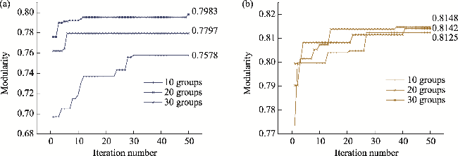
View original graphic|Download|PPT slide

Figure 16 Network modularity changing with iteration number (a. Baidu; b. AutoNavi)

Different intercity travel big data has its own characteristics and coverage, each facing issues related to insufficient detail disclosure. Nonetheless, on the whole, both Baidu and AutoNavi population migration data based on LBS are highly representative. The QAP analysis reveals a strong correlation in the intercity interactive network derived from Baidu, AutoNavi, and MP migration data. At the national scale, the correlation coefficient between the Baidu and AutoNavi networks stands at 0.874, while locally, this coefficient exceeds 0.90. This indicates that the two types of migration data can corroborate each other to a certain extent when representing the population movements. In other words, the migration data of Baidu and AutoNavi can effectively reflect the flow spatial structure of intercity interaction within regions. The correlation between the AutoNavi and MP networks is notably strong, with a correlation coefficient of 0.954, which is manifested in a closer network size, a more congruent hierarchical structure, and a more similar sequence of intercity interactive routes. Furthermore, the notable advantages of covering a comprehensive urban spatial scope and the long-term and sustained release, distinguish AutoNavi migration as superior for interpreting and analyzing the spatiotemporal characteristics and patterns of intercity interactions.

What’s more, by extracting the spatial structures of Baidu and AutoNavi’s intercity interactive networks at multiple levels, the study demonstrates a significant spatial dislocation effect between these two networks. This effect manifests as a spatial misalignment of network nodes, even when the node thresholds are consistent. Accordingly, this study evaluates the similarity between the two networks comprehensively, considering aspects such as node location, size, and local structure from a spatial association perspective. In terms of location similarity, the network nodes of both Baidu and AutoNavi exhibit high similarity within the four national-level urban agglomerations, with their spatial distributions aligning more consistently when the node threshold is set at 20. Regarding size similarity, as the node thresholds increase, the Baidu network perspective exhibits characteristics that are increasingly similar to those of the AutoNavi network. However, the spatial differentiation characteristics between the two networks are also significant. From the standpoint of structure similarity, the “social circles” of the local structures in both networks possess distinct characteristics. Within networks configured with node thresholds of 10, 20, and 30, higher convergence is exclusively evident in the Beijing-Tianjin-Hebei region, Northeast China, and the southeast coastal areas, respectively. Additionally, at a node threshold of 20, the distribution of similarity data for the local structure units in both networks exhibits greater consistency. Overall, the network with a node threshold of 20 demonstrates a higher degree of consistency in similarity measures between the two network structures.

Currently, research on intercity interaction relationships based on a single data source has attracted more and more critical attention from scholars (Hu et al., 2020b). For instance, Burger et al. (2014) suggested that urban networks exhibit multiplicity, with different spatial organizational structures observed from various evaluative perspectives. In other words, the choice of intercity datasets significantly influences the structure evaluation of urban networks. Although the exploration of spatial and coupling relationships between entities or virtual urban networks using multi-source data or multi-modal models has gained some scholarly attention, there are still few substantial achievements. Particularly in the integration of multi-source spatiotemporal big data, current efforts are often limited to advocacy, with little substantial progress. Recently, Luo and Chen (2024) developed an intercity population flow simulation model by integrating demographic and socio-economic data with Tencent migration big data. However, the accuracy of the results remains affected by biases inherent in big data. Obviously, the comparative study of intercity multi-source migration big data and their depicted urban networks herein aids in deepening the understanding of big data biases. Compared to the study by Xu et al. (2023), this study aims to reveal the spatial structure differences of intercity interactive networks from a more comprehensive perspective. It not only measured the similarities between nodes but also highlighted the overall differences and reliability of various data of flow. Additionally, the more in-depth quantitative measurement of similarity significantly distinguishes this study from general comparative analyses. For instance, Mu et al. (2024) conducted a comparative analysis between Baidu mobile big data and census data at the county level. Li et al. (2016) pointed out that Baidu and Tencent data had a good performance through a comparative analysis of the migration data derived from Baidu, Tencent, and Qihoo. This coincides with the findings of this study and can serve as empirical evidence for this research. However, as we know, the Tencent and Qihoo data sets are no longer updated. Therefore, a comparative analysis of the commonly used types of migration big data is greatly conducive to providing some insights and opinions for correctly understanding the regional interactions.

5.3 Limitations and implications

Inevitably, there are a few limitations in this study. In the first place, the disparities in data management strategies and openness mechanisms preclude the possibility of conducting more extensive comparative and coupling analyses. For example, in the spatiotemporal big data that characterizes China’s intercity mobility, Tencent population migration data is confined to the period from 2015 to 2019. Access to MP data in China remains challenging, and the predominant research outcomes associated with MP data are restricted to the transportation domain. Undoubtedly, the update of statistical data exhibits a significant lag, resulting in a pronounced lack of timeliness. Additionally, it is important to clarify that big data is not synonymous with complete data. Baidu, AutoNavi and MP migration data are all collected through the positioning function of the mobile client. Consequently, these data sets have inherent coverage limitations. They do not fully capture the movement of all individuals, particularly those without mobile phones, such as the elderly and children, whose mobility is not adequately represented. Moreover, migration data is significantly influenced by users’ personal preferences and behavior patterns. The different market shares held by Baidu and AutoNavi applications, along with variations in user profiles, data collection techniques, statistical methodologies, and release timelines, as well as the absence of corresponding high-precision data suitable for validation, not only collectively constrain the selection of research periods, but also the reason why different data sources may exhibit varying characteristics of network spatial structure. Furthermore, differences in analytical models, perspectives, and scales can significantly impact the accurate interpretation of group mobility phenomena based on migration big data (Liang et al., 2024). Specifically, using various analytical models, such as the gravity model and radiation model, may reveal differing spatial differentiation characteristics in intercity interactive networks. Further analysis of migration big data from a global or local perspective often remains too general, making it challenging to fully capture the complexity and diversity of intercity interactive networks. Varying scales of analysis may lead to misjudgments regarding the reliability and analysis efficiency of multi-source migration big data. In short, ignoring these data biases may lead to misunderstandings of spatial interaction relationships or patterns.

Furthermore, it should be realized that relying only on a single data source to analyze spatial interaction relationships or formulate regional development strategies may lead to a series of risks and uncertainties. In other words, these differences might impact policy or urban planning decisions. For example, interpreting regional association only through Baidu migration data may overemphasize the high-level cross-regional ability, thus ignoring the importance and role of marginal city nodes in the network, leading to the lack of comprehensive understanding of regional networks. On the contrary, if only AutoNavi migration data is used as the analysis basis, it may lead to underestimation of the actual intensity of cross-regional interaction. Therefore, to understand the regional interaction relationships more accurately and formulate scientific and reasonable regional development strategies, it is necessary and advocated to integrate comprehensive analysis of multi-source data and models (Liao et al., 2023; Luo and Chen, 2024).

Accordingly, it is hoped that government agencies could create a data platform in the future, integrating LBS, mobile phone big data and official authoritative data of transportation departments, breaking down data barriers. This integration aims to enhance research on the identification of spatial structures and regional interactions using multi-source spatiotemporal big data, thereby facilitating more precise and authoritative recommendations for regional collaboration and service decisions. In the information age, big data plays an irreplaceable role in decision support, driving innovation, optimizing management, and improving competitiveness. Relevant departments should prioritize and actively promote the application of spatiotemporal big data, with the aim of accurately identifying “hot spots” through the utilization of massive emerging spatiotemporal data sets generated in real-time. In particular, it is crucial to have a comprehensive understanding of the deviation in multi-source big data and leverage its unique advantages. By employing advanced computing technology and data mining methods, the decision-making process will be expedited and innovated through data fusion or effective replacement strategies. This will lead to improved efficiency and enhanced decision-making in the utilization of spatiotemporal big data. The objective of this endeavor is to enhance overall response efficiency and optimize the quality of geographic information decision-making, thereby better serving the improvement of urban infrastructure, the optimal management of transportation system, and the effect prevention and response to public safety emergencies.

6 Conclusions

This study aims to elucidate the variances in spatial structure of intercity interactive networks at multiple levels represented by multi-source migration flow data. At the first place, intercity interactive networks were constructed using the multimodal population migration data, including the BMI, AMI, and MP. Subsequently, the multi-hierarchical spatial structures of networks were extracted. Moreover, the study conducts a comparative analysis of the spatial patterns and the structure similarity characteristics of these networks, examining them from both overarching and localized viewpoints. The main conclusions are as follows:

(1) The intercity interactive networks in China, as delineated by Baidu and AutoNavi migration flows respectively, exhibit a high degree of structure equivalence. The correlation coefficient between these two types of networks is 0.874. Both networks display a pronounced spatial polarization trend and hierarchical structure. This is reflected in the distinct core and peripheral structures, as well as in the importance and influence of various nodes within the networks. In addition to the pronounced density disparity across the Hu Line, with the southeast half exhibiting dense and the northwest half notably sparse, there are prominent high-hierarchical network structures centralized around the core cities within four major national-level urban agglomerations, such as the Pearl River Delta, the Yangtze River Delta, the Beijing-Tianjin-Hebei, and the Chengdu-Chongqing regions.

(2) Nevertheless, the differences between the two networks cannot be ignored. The Baidu intercity interactive network exhibits pronounced cross-regional effects, which can overcome geographical barriers to a large extent. The high-level interactions in the network are characterized by a “rich-club” phenomenon, where core cities manifest a more significant radiation effect. However, the AutoNavi intercity interactive network presents a more marked distance attenuation effect. Its high-level interactions display a gradient distribution pattern. Notably, there is a significant correlation between the AutoNavi and the MP networks at the local scale, as evidenced by a high correlation coefficient of 0.954.

(3) The relationships of “spatial dislocation” were observed within the spatial structures of the Baidu and AutoNavi intercity interactive networks at various levels. However, when examined through the lens of network similarity metrics based on a comprehensive association perspective, the results indicate a relatively high similarity and consistency between the perspectives of the two networks. Regarding node location, network nodes situated within the four major national-level urban agglomerations exhibit a high matching. With respect to node size, nodes within the Baidu network present a more analogous scale of interaction relative to those in the AutoNavi network; nevertheless, they display pronounced spatial differentiation characteristics. Concerning local structure, the “circle of friends” of both types of networks demonstrates greater consistency within the Beijing-Tianjin-Hebei region, as well as Northeast and Southeast China.

Data availability

The data used and analyzed during the current study are available from the corresponding author on reasonable request.

Conflicts of interest

The authors declare no conflict of interest.

References

Publishing order | Descend order by publishing year | Descend order by cited within

[1]	Bao X G, Ji P, Lin W et al., 2021. The impact of COVID-19 on the worldwide air transportation network. Royal Society Open Science, 8(11): 210682.

[2]	Burger M, Knaap B, Wall R. 2014. Polycentricity and the multiplexity of urban networks. European Planning Studies, 22(4): 816-840.

[3]	Castells M. 1996. Rise of the Network Society: The Information Age: Economy, Society and Culture. Oxford: Black-well.

[4]	Chen Y Z, Gong Z Y, Ma Q W et al., 2023. Exploring the spatiotemporal relationships between search flows and travel flows. Transactions in GIS, 27(5): 1338-1356.

[5]	Fan J Q, Han F, Liu H, 2014. Challenges of big data analysis. National Science Review, 1(2): 293-314.

[6]	Fang H M, Wang L, Yang Y, 2020. Human mobility restrictions and the spread of the Novel Coronavirus (2019-nCoV) in China. Journal of Public Economics, 191: 104272.

[7]	Gao P, Qi W, Liu S H et al., 2023. Moving to a healthier city? An analysis from China’s internal population migration. Frontiers in Public Health, 11: 1132908.

[8]	Gao S, Liu Y, Wang Y L et al., 2013. Discovering spatial interaction communities from mobile phone data. Transactions in GIS, 17(3): 463-481.

[9]	Gou W S, Huang S Y, Chen Q H et al., 2020. Structure and dynamic of global population migration network. Complexity, 2020: 4359023.

[10]	Haraguchi M, Nishino A, Kodaka A et al., 2022. Human mobility data and analysis for urban resilience: A systematic review. Environment and Planning B: Urban Analytics and City Science, 49(5): 1507-1535.

[11]	He J Y, Wei Y, Yu B L, 2023. Geographically weighted regression based on a network weight matrix: A case study using urbanization driving force data in China. International Journal of Geographical Information Science, 37(6): 1209-1235.

[12]	Hu T, Guan W W, Zhu X Y et al., 2020a. Building an open resources repository for COVID-19 research. Data and Information Management, 4(3): 130-147.

[13]	Hu T, Wang S Q, She B et al., 2021. Human mobility data in the COVID-19 pandemic: Characteristics, applications, and challenges. SSRN Electronic Journal, 14(9): 1126-1147.

[14]	Hu X Q, Wang C, Wu J J et al., 2020b. Understanding interurban networks from a multiplexity perspective. Cities, 99: 102625.

[15]	Krackardt D, 1987. QAP partialling as a test of spuriousness. Social Networks, 9(2): 171-186.

[16]	Lao X, Zhang X L, Shen T Y et al., 2016. Comparing China’s city transportation and economic networks. Cities, 53: 43-50.

[17]	Li J W, Ye Q Q, Deng X K et al., 2016. Spatial-temporal analysis on Spring Festival Travel Rush in China based on multisource big data. Sustainability, 8(11): 1184.

[18]	Li M Z, Li H C, Wang K et al., 2023. Dynamic network relationship between transportation and urban economy: A case study of China’s high-speed rail as a new transportation technology. Research in Transportation Economics, 102: 101360.

[19]	Liang X F, Hidalgo C A, Balland P-A et al., 2024. Intercity connectivity and urban innovation. Computers, Environment and Urban Systems, 109: 102092.

[20]	Liao C C, Hong W Y, Li Y X et al., 2023. Potential and real spatial models: Differences and response characteristics from the perspective of flow. Cities, 138: 104358.

[21]	Lu D B, Xiao W, Xu G Y et al., 2021a. Spatiotemporal patterns and influencing factors of human migration networks in China during COVID-19. Geography and Sustainability, 2(4): 264-274.

[22]	Lu X, Tan J, Cao Z Q et al., 2021b. Mobile phone-based population flow data for the COVID-19 outbreak in mainland of China. Health Data Science, 2021: 9796431.

[23]	Luo M, Chen Y M. 2024. Simulating inter-city population flows based on graph neural networks. Geocarto International, 39(1): 2331223.

[24]	Meng H, Huang X J, Mao X Y et al., 2023. The formation and proximity mechanism of population flow networks under multiple traffic in China. Cities, 136: 104211.

[25]	Mu X F, Fang C L, Yang Z Q et al., 2022. Impact of the COVID-19 epidemic on population mobility networks in the Beijing-Tianjin-Hebei urban agglomeration from a resilience perspective. Land, 11(5): 675.

[26]	Mu X Y, Zhang X H, Yeh A G-O et al., 2024. Evaluating the representativeness of mobile big data: A comparative analysis between China’s mobile big data and census data at the county level. Applied Geography, 166: 103260.

[27]	Newman M E J, 2006. Modularity and community structure in networks. Proceedings of the National Academy of Sciences, 103(23): 8577-8582.

[28]	Pan J H, Lai J B. 2019. Spatial pattern of population mobility among cities in China: Case study of the National Day plus Mid-Autumn Festival based on Tencent migration data. Cities, 94: 55-69.

[29]	Shi W Z, Zhang A S, Zhou X L et al., 2018. Challenges and prospects of uncertainties in spatial big data analytics. Annals of the American Association of Geographers, 108(6): 1513-1520.

[30]	Wang H, Zhang X Y, Zhang X Y et al., 2024. Understanding coordinated development through spatial structure and network robustness: A case study of the Beijing-Tianjin-Hebei region. Journal of Geographical Sciences, 34(5): 1007-1036.

[31]	Wang X W, Liu C, Mao W L et al., 2014. Tracing the largest seasonal migration on earth. Physics, doi: 10.48550/arXiv.1411.0983.

[32]	Wei Y, Song W, Xiu C L et al., 2018. The rich-club phenomenon of China’s population flow network during the country’s spring festival. Applied Geography, 96: 77-85.

[33]	Wu Y M, Wang L, Fan L H et al., 2020. Comparison of the spatiotemporal mobility patterns among typical subgroups of the actual population with mobile phone data: A case study of Beijing. Cities, 100: 102670.

[34]	Xiu Y X, Li W D, Xi J Y et al., 2021. OD-HyperNet:A data-driven hyper-network model for origin-destination matrices completion using partially observed data. LISS 2020. Singapore: Springer Singapore, 335-350.

[35]	Xu H L, Cheng L, 2016. The QAP weighted network analysis method and its application in international services trade. Physica A: Statistical Mechanics and Its Applications, 448: 91-101.

[36]	Xu Y S, Zhang H P, Li Z H et al., 2023. Integration of migration and attention flow data to reveal association of virtual-real dual intercity network structure. Cities, 143: 104614.

[37]	Yang L J, Wang J, Yang Y C, 2022. Spatial evolution and growth mechanism of urban networks in western China: A multi-scale perspective. Journal of Geographical Sciences, 32(3): 517-536.

[38]	Ye S S, Qian Z, 2021. The economic network resilience of the Guanzhong Plain City Cluster, China: A network analysis from the evolutionary perspective. Growth and Change, 52(4): 2391-2411.

[39]	Zhang J, Hao Q, Chen X M et al., 2022. Exploring spatial network structure of the metropolitan crcle based on multi-source big data: A case study of Hangzhou metropolitan circle. Remote Sensing, 14(20): 5266.

[40]	Zhang R, Pan J H, Lai J B, 2021. Network structure of intercity trips by Chinese residents under different travel modes: A case study of the Spring Festival Travel Rush. Complexity, 2021: 1-19.

[41]	Zhang W J, Fang C Y, Zhou L et al., 2020a. Measuring megaregional structure in the Pearl River Delta by mobile phone signaling data: A complex network approach. Cities, 104: 102809.

[42]	Zhang W Y, Derudder B, Wang J H et al., 2020b. An analysis of the determinants of the multiplex urban networks in the Yangtze River Delta. Tijdschrift voor Economische en Sociale Geografie, 111(2): 117-133.

[43]	Zhao Y T Z, Gao Y, 2024. Spatial patterns and trends of inter-city population mobility in China: Based on Baidu migration big data. Cities, 151: 105124.

[44]	Zheng L F, Long F J, Zhang S, 2020. Comparison of the spaces of call and traffic flows: An empirical study of Qianzhong urban region, China. Cities, 107: 102927.

[45]	Zhou T, Huang B, Liu X Q et al., 2020. Spatiotemporal exploration of Chinese Spring Festival population flow patterns and their determinants based on spatial interaction model. ISPRS International Journal of Geo-Information, 9(11): 670.

[46]	Zhou X X, Zhang H P, Ye X Y, 2024a. A multi-hierarchical method to extract spatial network structures from large-scale origin-destination flow data. International Journal of Geographical Information Science, 38(3): 577-602.

[47]	Zhou Y, Zheng W S, Wang X F et al., 2024b. Urban economic efficiency under the interactive effect of urban hierarchy and connection networks in China. Journal of Geographical Sciences, 34(12): 2315-2332.

Options

Outlines

模态框（Modal）标题

Abstract

Cite this article

1 Introduction

2 Study area and data description

Figure 1 Locations of major cities in China

Table 1 A sample of Baidu intensity index

Table 2 A sample of Baidu proportion index

Figure 2 Schematic of calculating intercity travel scale index based on intensity index and proportion index

Table 3 A sample of AMI data

Table 4 A sample of mobile phone data from Wuhan to other cities in China

Table 5 Characteristics of Baidu, AutoNavi and mobile phone intercity population migration data

3 Research framework and methods

3.1 Research framework

Figure 3 Research framework for revealing the differences in spatial structure of intercity interactive networks

3.2 Methods

3.2.1 Complex network analysis

3.2.2 Network spatial structure extraction

3.2.3 Measuring similarity in network structures

Figure 4 Schematic of location projection and similarity measuring in network structures (a. Baidu network; b. AutoNavi network; c. Euclidean distance based on the location of nodes; d. Nodes and their size; e. Local network structure)

4 Results

4.1 Overall characteristic and correlation of intercity interactive networks

Figure 5 Spatial pattern of intercity interactive networks in China (a. Baidu; b. AutoNavi)

Figure 6 Distribution of distance in intercity interactive scale in China

Figure 7 The intercity interaction strength of urban nodes (a-b. Distribution of urban outflow and inflow scales; c-d. Top 20 cities of total scale)

Table 6 Top 20 routes of Wuhan’s intercity outflow network from Baidu, AutoNavi and MP migration data

Table 7 QAP correlation analysis of intercity interactive networks

4.2 Spatial structure of intercity interactive networks at different levels

Figure 8 Spatial structure of intercity interactive network in China at different levels (a-c. Baidu networks with 10, 20, 30 nodes; d-f. AutoNavi networks with 10, 20, 30 nodes)

Figure 9 Statistics of sub-nodes for each final node in the intercity interactive networks at different levels (a-c. Baidu; d-f. AutoNavi)

4.3 Spatial structure similarities of intercity interactive networks

4.3.1 Node location similarity

Figure 10 Node location similarity (nodes and links corresponding to Baidu and AutoNavi network are blue and yellow, respectively) (a. 10 nodes; b. 20 nodes; c. 30 nodes)

Figure 11 Violin plot of node location similarity (a. 10 nodes; b. 20 nodes; c. 30 nodes)

4.3.2 Node size similarity

Figure 12 Node size similarity (nodes and links corresponding to Baidu and AutoNavi network are blue and yellow, respectively) (a. 10 nodes; b. 20 nodes; c. 30 nodes)

Figure 13 Violin plot of node size similarity (a. 10 nodes; b. 20 nodes; c. 30 nodes)

4.3.3 Local structure similarity

Figure 14 Local structure similarity (nodes and links corresponding to Baidu and AutoNavi network are blue and yellow, respectively) (a. 10 nodes; b. 20 nodes; c 30 nodes)

Figure 15 Violin plot of local structure similarity (a. 10 nodes; b. 20 nodes; c. 30 nodes)

5 Discussion

5.1 Significances and contributions

5.2 Explanations and comparisons

Figure 16 Network modularity changing with iteration number (a. Baidu; b. AutoNavi)

5.3 Limitations and implications

6 Conclusions

Data availability

Conflicts of interest

References