
Journal of Geographical Sciences >
Global submarine cable network and digital divide
|
Ma Xueguang (1979-), PhD and Professor, specialized in ocean security and global ocean governance. E-mail: maxg@nankai.edu.cn |
Received date: 2025-01-24
Accepted date: 2025-04-24
Online published: 2025-08-28
Supported by
National Natural Science Foundation of China(42371175)
As the most important large-scale communication infrastructure in the world today, submarine cable can profoundly reflect the global Internet communication pattern, and is of great significance for understanding the global digital divide. We used multi-scale and network analysis methods to depict the distribution pattern, network structure and spatio-temporal evolution of global submarine cables at the national and landing point scales, in order to analyze the current situation, challenges and main directions of global digital divide governance. Results show that: (1) spatial distribution of global submarine cables is unbalanced, the United States and Europe are the concentrated distribution areas of submarine cables and global information flow centers; (2) core connections of the global submarine cable network are only composed of a tiny minority of countries or regions or landing points, and have strong geographical proximity and clustered-type characteristic, noting that multitudinous landing points of developed countries are at the semi-periphery or even periphery of the network; (3) submarine cables can alleviate the global digital divide through the three paths of infrastructure universalization, digital ecosystem reconstruction and economic empowerment, and the global digital divide governance still faces the dilemma of the differences in digital strategy development and the lack of a governance system. However, due to the increasingly important position of cities in developing countries in the international communication pattern, the global digital divide problem is being alleviated.
MA Xueguang , JIANG Ce . Global submarine cable network and digital divide[J]. Journal of Geographical Sciences, 2025 , 35(6) : 1204 -1232 . DOI: 10.1007/s11442-025-2364-x
Table 1 The definition of CNA indicators |
| Indicator | Formula | Specific meaning | Representational meaning |
|---|---|---|---|
| Degree centrality | $P_{r}=\frac{D_{r}}{N-1}$ (1) | Dr is the number of nodes connected to node r, and N is the total number of all nodes (the same below). | Representing the number of nodes directly related to a node, which can reflect the direct accessibility of nodes in the network. |
| Closeness centrality | $C_{c}(i)=\frac{N-1}{\sum_{j \in V_{N}, j \neq i} \operatorname{Dist}(i, j)}$ (2) | Dist(i,j) is the shortest path connecting nodes i and j, and VN is the point set in the network (the same below). | Representing the average length of the shortest path from a node to all other nodes, which can reflect the relative accessibility of nodes in the network. |
| Betweenness centrality | $C_{b}(i)=\frac{2 \sum_{j \neq k \neq i \in V_{N}} \frac{g_{j k}(i)}{g_{j k}}}{(N-1)(N-2)}$ (3) | gjk(i) is the number of shortest paths between other nodes jk through node i, and gjk is the number of shortest paths between other nodes jk. | Representing the probability that the shortest path between other nodes needs to pass through a certain node, which can reflect the transfer and cohesion functions of nodes in the network. |
| Eigenvector centrality | $C_{E}(i)=\frac{1}{\lambda} \sum_{j} W_{i j} C_{E}(j)$ (4) | Wij is the connection strength between nodes i and j, and λ is taken as the largest eigenvalue. | Representing the position of the node through close connection with the hub node. |
| Connectivity | NA | NA | Representing the degree of internal and external connection of nodes. Due to the complexity of submarine cable data processing, we define the connectivity of nodes as the direct arrival of the initial station to the destination. |
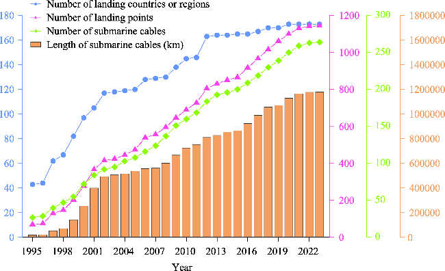
Figure 1 Changes in the number, length, landing countries or regions, and landing points of global submarine cables from 1995 to 2023 |
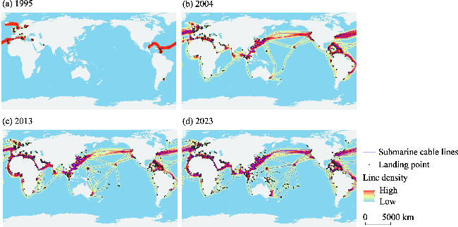
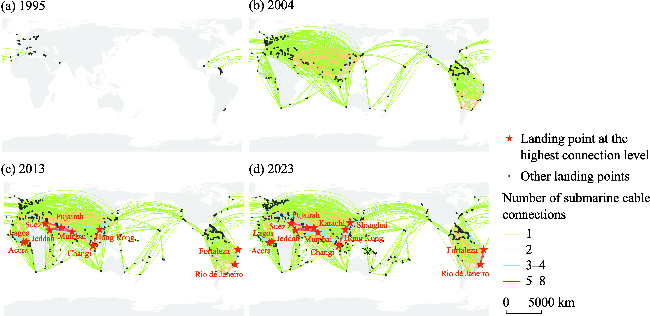
Figure 2 Distribution pattern of global submarine cable lines and their density in 1995 (a), 2004 (b), 2013 (c) and 2023 (d) |
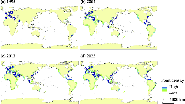
Figure 3 The point density distribution of global submarine cable landing points in 1995 (a), 2004 (b), 2013 (c) and 2023 (d) |
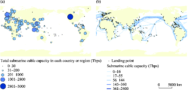
Figure 4 Distribution of total submarine cable capacity in each country or region in 2023 (a); The capacity of submarine cable connections between landing points in 2023 (b) |
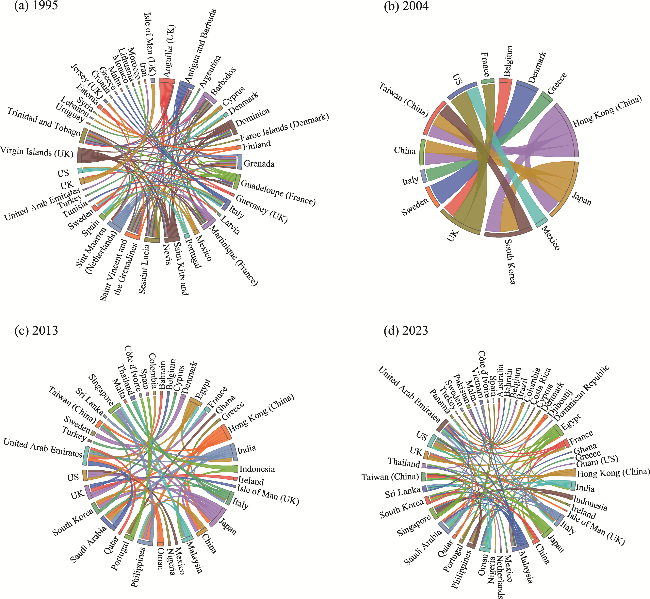
Figure 5 The core connection pattern of number of submarine cable connections between countries or regions in 1995 (a), 2004 (b), 2013 (c) and 2023 (d). Except for 1995, only country or region pairs with 4 or more connections are shown for the remaining three years. |
Figure 6 The distribution pattern of submarine cable connections between landing points in 1995 (a), 2004 (b), 2013 (c) and 2023 (d). The landing points at the highest connection level are marked in red. |
Table 2 The centrality of the submarine cable network nodes |
| S/N | Year | Node | Degree centrality | Node | Closeness centrality | Node | Betweenness centrality | Node | Eigenvector centrality |
|---|---|---|---|---|---|---|---|---|---|
| 1 | 2004 | Hong Kong | 8.785 | Lowestoft | 2.000 | Hollywood | 18.270 | Hong Kong | 1.000 |
| 2 | 2004 | Shanghai | 8.311 | Doha | 1.998 | Mazara del Vallo | 13.649 | Shanghai | 0.998 |
| 3 | 2004 | Bantangas | 7.015 | Alsgarde | 1.995 | Cancún | 11.870 | Penang | 0.948 |
| 4 | 2004 | Penang | 6.714 | Kristinelund | 1.993 | Palermo | 10.708 | Alexandria | 0.941 |
| 5 | 2004 | Sesimbra | 6.693 | Island Park | 1.993 | Fortaleza | 10.506 | Jeddah | 0.941 |
| 6 | 2004 | Fangshan | 6.571 | Plerin | 1.992 | Shima | 8.938 | Fujairah | 0.941 |
| 7 | 2004 | Alexandria | 6.222 | Aldeburgh | 1.990 | Le Lamentin | 6.000 | Suez | 0.940 |
| 8 | 2004 | Fujairah | 5.865 | Domburg | 1.988 | Chania | 5.476 | Geoje | 0.940 |
| 9 | 2004 | Jeddah | 5.588 | Otranto | 1.987 | Brookhaven | 4.000 | Mumbai | 0.940 |
| 10 | 2004 | Geoje | 5.001 | Aetos | 1.987 | Sesimbra | 3.157 | Satun | 0.940 |
| 1 | 2013 | Mumbai | 11.112 | Lowestoft | 2.446 | Hollywood | 22.102 | Mumbai | 1.000 |
| 2 | 2013 | Jeddah | 10.934 | Alsgarde | 2.443 | Mazara del Vallo | 17.087 | Jeddah | 0.990 |
| 3 | 2013 | Fujairah | 9.750 | Kristinelund | 2.442 | Palermo | 15.737 | Suez | 0.950 |
| 4 | 2013 | Hong Kong | 9.200 | Island Park | 2.437 | Cancún | 13.164 | Fujairah | 0.943 |
| 5 | 2013 | Suez | 8.919 | Plerin | 2.437 | Hong Kong | 12.024 | Hong Kong | 0.903 |
| 6 | 2013 | Shanghai | 7.332 | Aldeburgh | 2.435 | Le Lamentin | 10.552 | Shanghai | 0.879 |
| 7 | 2013 | Sesimbra | 7.052 | Domburg | 2.434 | Mumbai | 8.442 | Alexandria | 0.879 |
| 8 | 2013 | Alexandria | 6.011 | Otranto | 2.432 | Fujairah | 7.806 | Satun | 0.866 |
| 9 | 2013 | Penmarch | 5.681 | Aetos | 2.432 | Fortaleza | 7.262 | Sesimbra | 0.835 |
| 10 | 2013 | Satun | 5.354 | Poti | 2.432 | Chania | 5.598 | Geoje | 0.834 |
| 1 | 2023 | Mumbai | 13.186 | Lowestoft | 2.719 | Morro Bay | 34.464 | Mumbai | 1.000 |
| 2 | 2023 | Fujairah | 12.212 | Alsgarde | 2.717 | Hollywood | 32.010 | Jeddah | 0.989 |
| 3 | 2023 | Jeddah | 12.207 | Kristinelund | 2.716 | Mazara del Vallo | 28.100 | Fujairah | 0.985 |
| 4 | 2023 | Hong Kong | 11.993 | Island Park | 2.716 | Palermo | 24.387 | Hong Kong | 0.908 |
| 5 | 2023 | Tuas | 10.159 | Plerin | 2.715 | Cancún | 22.071 | Karachi | 0.901 |
| 6 | 2023 | Suez | 9.788 | Aldeburgh | 2.713 | Hong Kong | 17.846 | Suez | 0.882 |
| 7 | 2023 | Karachi | 7.756 | Domburg | 2.713 | Hillsboro | 16.000 | Satun | 0.871 |
| 8 | 2023 | Penang | 6.755 | Otranto | 2.713 | Sydney | 15.500 | Tuas | 0.857 |
| 9 | 2023 | Shanghai | 6.613 | Aetos | 2.712 | San Juan | 11.019 | Penang | 0.853 |
| 10 | 2023 | Satun | 6.398 | Poti | 2.711 | Mersing | 9.707 | Alexandria | 0.806 |
Note: Only the top 10 nodes in every year are listed, taking three decimal places. Due to the limited number of landing points and the absence of a complex network in 1995, this table does not report centrality indicators for 1995. |
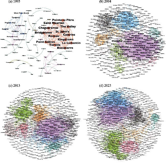
Figure 7 Spatial structure of submarine cable connection network between landing points in 1995 (a), 2004 (b), 2013 (c) and 2023 (d). Different node sizes represent different centrality, and different colors represent different communities. |
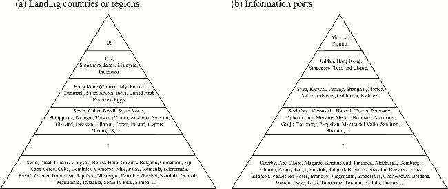
Figure 8 Global submarine cable landing countries or regions (a); landing points level structure (b) |
| [1] |
|
| [2] |
|
| [3] |
|
| [4] |
|
| [5] |
|
| [6] |
|
| [7] |
|
| [8] |
|
| [9] |
|
| [10] |
|
| [11] |
|
| [12] |
|
| [13] |
|
| [14] |
|
| [15] |
|
| [16] |
|
| [17] |
|
| [18] |
|
| [19] |
|
| [20] |
|
| [21] |
|
| [22] |
|
| [23] |
|
| [24] |
Government of Cambodia, 2021. Cambodia Digital Economy and Society Policy Framework 2021-2035. Ministry of Economy and Finance, Government of Cambodia.https://mef.gov.kh/download-counter?post=7116.
|
| [25] |
|
| [26] |
|
| [27] |
|
| [28] |
|
| [29] |
|
| [30] |
|
| [31] |
|
| [32] |
|
| [33] |
|
| [34] |
|
| [35] |
|
| [36] |
|
| [37] |
|
| [38] |
|
| [39] |
|
| [40] |
|
| [41] |
|
| [42] |
|
| [43] |
|
| [44] |
|
| [45] |
|
| [46] |
|
| [47] |
|
| [48] |
|
| [49] |
|
| [50] |
|
| [51] |
|
| [52] |
|
| [53] |
|
| [54] |
|
| [55] |
|
| [56] |
|
| [57] |
|
| [58] |
|
| [59] |
|
| [60] |
|
| [61] |
|
| [62] |
|
| [63] |
|
| [64] |
|
| [65] |
|
| [66] |
|
| [67] |
|
| [68] |
TeleGeography, 2023. Submarine Cable Map. Available at: https://www2.telegeography.com/.
|
| [69] |
|
| [70] |
|
| [71] |
|
| [72] |
|
| [73] |
|
| [74] |
|
| [75] |
|
| [76] |
|
| [77] |
|
| [78] |
|
| [79] |
|
| [80] |
|
| [81] |
|
/
| 〈 |
|
〉 |