Research Articles

Enhancing flood risk assessment in northern Morocco with ‎tuned machine learning and advanced geospatial ‎techniques

  • MOUTAOUAKIL Wassima 1 ,
  • HAMIDA Soufiane , 2, 3, * ,
  • SALEH Shawki 1 ,
  • LAMRANI Driss 1 ,
  • MAHJOUBI Mohamed Amine‎ 1 ,
  • CHERRADI Bouchaib 1, 2, 4 ,
  • RAIHANI Abdelhadi 1
Expand
  • 1. EEIS Laboratory, ENSET of Mohammedia, Hassan II University of Casablanca, Mohammedia, Morocco
  • 2. 2IACS Laboratory, ENSET of Mohammedia, Hassan II University of Casablanca, Mohammedia, Morocco
  • 3. GENIUS Laboratory, SupMTI of Rabat, Rabat, Morocco
  • 4. STIE Team, CRMEF Casablanca-Settat, Provincial Section of El Jadida, El Jadida, Morocco
*HAMIDA Soufiane, E-mail:

Received date: 2024-03-21

  Accepted date: 2024-09-11

  Online published: 2025-01-16

Abstract

Mapping floods is crucial for effective disaster management. This study focuses on flood assessment in northern Morocco, specifically Tangier, Tetouan, and Larache. Due to the lack of a comprehensive flood inventory map, we used unsupervised learning techniques, such as K-means clustering and fuzzy logic algorithms, to predict flood-prone areas. We identified nine conditioning factors influencing flood risk: elevation, slope, aspect, plan curvature, profile curvature, land use, soil type, normalized difference vegetation index (NDVI), and topographic position index (TPI). Using Landsat-8 imagery and a Digital Elevation Model (DEM) within a Geographic Information System (GIS), we analyzed topographic and geo-environmental variables. K-means clustering achieved silhouette scores of 0.66 in Tangier and 0.70 in Tetouan, while the fuzzy logic method in Larache produced a Davies-Bouldin Index (DBI) score of 0.35. The maps classified flood risk levels into low, moderate, and high categories. This research demonstrates the integration of machine learning and remote sensing for predicting flood-prone areas without existing flood inventory maps. Our findings highlight the main factors contributing to flash floods and assess their impact, enhancing the understanding of flood dynamics and improving flood management strategies in vulnerable regions.

Cite this article

MOUTAOUAKIL Wassima , HAMIDA Soufiane , SALEH Shawki , LAMRANI Driss , MAHJOUBI Mohamed Amine‎ , CHERRADI Bouchaib , RAIHANI Abdelhadi . Enhancing flood risk assessment in northern Morocco with ‎tuned machine learning and advanced geospatial ‎techniques[J]. Journal of Geographical Sciences, 2024 , 34(12) : 2477 -2508 . DOI: 10.1007/s11442-024-2301-4

1 Introduction

Flash floods are one of the most common natural hazards worldwide, causing severe damage (Costache, 2019). At the same time, many efforts were carried out to identify areas susceptible to flooding. Given this situation, Morocco amplified its efforts to map this natural hazard. According to the official report produced by the Ministry * , are 313 locations prone to flooding across 10 administrative regions of Morocco. The flood risk levels are categorized based on water levels and flow velocities, with specific thresholds defining low, mean, and high-risk levels. Low risk corresponds to water velocity less than 0.50 meters per second, mean risk to velocities between 0.50 and 1 meter per second, and high risk to velocities exceeding 1 meter per second. The report provides a quantitative assessment where 23% of the locations are classified as very high risk, 41% as high potential for flooding, 34% as medium risk, and 2% as moderate risk. This data indicates that approximately 64% of the surveyed sites face significant flood risk. The regions of Marrakech-Safi and Fes-Meknes achieved the highest score of 51 flooded sites, followed by Sous-Massa with 50 flooded locations and Tangier-Tetouan-Al Houciema with a rate of 44. By analyzing the topography in Morocco (Teixell et al., 2003), is divided into three areas: the northern coastal plain along the Mediterranean, which Rif Mountains varying in elevation, the rich plateaus and lowlands lying between the three parallel ranges of the Atlas Mountains and the Mediterranean in the northeast this variation occupies a primary importance to detect factors that lead to flood.
Taking this into account, this field of research has seen a revolution in terms of methods applied to achieve these goals. It has evolved from traditional techniques based on statistical functions, which have limitations in managing the complexity of data related to flood conditioning factors (Xu et al., 2022; Thankappan et al., 2023), to the integration of artificial intelligence and remote sensing. The advantages of these new technologies are the enhancement of prediction accuracy and the ability to consume large amounts of data automatically. Therefore, it is essential to explore types of ML introduced in scientific research, especially unsupervised learning, and the most famous algorithms used for flood assessment are K-means clustering and fuzzy logic methods. Moreover, the map of flood susceptibility represents a challenging task as we need to identify the conditioning factors that lead to its occurrence (Talukdar et al., 2020), namely elevation, slope, TPI, aspect, NDVI, LU, soil type, plan curvature, and profile curvature. To achieve these aims, this study combines the ML approaches in the GIS environment using remote sensing sources to mitigate flood impacts over the long term (Balestra et al., 2022).
In the same context, the analysis of topographic, climatic, historic, and hydrological factors guides our work to adopt the northern region of Morocco as the principal area of study. With 44 sites, 27 pose a significant flood risk. Taking into consideration, the population density, touristic and economic aspects of these regions, it is crucial to implement an assessment map of flood hazards to mitigate their destructive damage (Rincón et al., 2018). According to Mosavi et al. (2018), four criteria determine the approach to guide the study in this field of research, namely the source and the type of conditioning factors, prediction type, ML used, and the result obtained. These four parameters are related to each other, which means that to choose the type of flood source variables, it is primordial to define the type of prediction, whether it is generated for a long time or a short time. For instance, if we want a flood prediction for a short time or flash floods, we can use rainfall or melting snow, but for a long-term prediction, we can use soil moisture and rainfall. On the other hand, the choice of ML depends as well on the type of prediction applied. In our case study, the main aim is to locate the region with high flood risk, challenging the lack of a large-scale flood inventory map and data imagery within a short period.
Floods are widely recognized as one of the most pervasive and destructive natural disasters worldwide. For example, in Morocco, floods rank second only to earthquakes in terms of the number of injuries and fatalities they cause (Meliho et al., 2021, 2022). There are numerous factors contributing to flooding, including climate change, rapid urban development, alterations in drainage network morphology, limited infiltration capacity, and insufficient land storage, particularly during periods of intense rainfall (Bouramtane et al., 2021). In response to this pressing need for an effective flood susceptibility map to mitigate the impact of this natural hazard, numerous studies have been conducted in Morocco and other countries, focusing particularly on regions with a documented history of recurrent flooding (Talha et al., 2019; Bouramtane et al., 2021; Meliho et al., 2022; Sellami et al., 2022; Li et al., 2023).
In different research, the application of new techniques to map flood susceptibility shows relevant results working with ML approaches with remote sensing and GIS instead of traditional methods. To mention a few, as stated in (Sellami et al., 2022), five ML methods were applied, namely Support Vector Machine (SVM), Logistic Regression (LR), Random Forest (RF), Naïve Bayes (NB), and Artificial Neural Network (ANN), on a dataset of 1101 points in Tetouan, Morocco, including nine conditioning factors such as elevation, slope, aspect, LU/LC, Stream Power Index (SPI), plan curvature, profile curvature, TPI, and Topographic Witness Index (TWI). The RF achieved the highest accuracy score of 96% as a result, mapping flood flash susceptibility into five classes: low, lowest, moderate, high, and highest. According to this study, 36% of this area shows a high vulnerability to flooding due to its proximity to the “Oued Martil”. In the same context in the northern region of Morocco, specifically in Tangier (Bouramtane et al., 2021), the author employed four supervised ML models: SVM, LR, Classification and Regression Trees (CART), and Linear Discriminant Analysis (LDA) to delineate flood-prone areas. This assessment was grounded in two categories of flood factors: geo-environmental and socio-environmental causes. The findings unveiled that out of the 13 principal components, six exhibited significant influence on flood occurrence. It should be noted that CART and SVM demonstrated impressive accuracy, achieving a remarkable score of 91.6%. Furthermore, fuzzy inference and AHP were combined to predict flash floods in Guelmim, Morocco (Talha et al., 2019). The dataset contains seven conditioning factors, namely, soil measurement index (SMI), drainage density, rainfall, LU/LC, altitude, slope, and soil type. Using AHP to calculate the weight of each factor, then scaling them between 0 and 1 using Fuzzy membership to be fed to the Fuzzy Analytical Hierarchical Process (FAHP), the last technique aims to multiply the fuzzy results with the AHP weight. The finding is a map of flood susceptibility that consists of three classes: low, moderate, and high. The high risk of flooding was defined relative to weight factors. Thus, a high value of SMI leads to a rate of 37% flood occurrence, where low drainage density and low rainfall highlight a low to moderate risk of flooding. Regarding this study, around 47.57% of zones were characterized by high risk, and they were detected close to rivers and at the outlet of watersheds. Nevertheless, in different areas of study, the same observations were found (Meliho et al., 2022). This research was conducted in the Ourika Watershed of Morocco, applying 16 conditioning factors related to hydrology, including drainage density, flow accumulation, flow direction, as well as commonly used factors such as curvature, elevation, and slope. The primary objective was to employ four ML models: K-nearest neighbor (KNN), ANN, RF, and X-gradient Boost (XGB) to produce a flood susceptibility map. The results indicate that RF and XGB achieved the highest level of accuracy. Consequently, the flood susceptibility map generated reveals that 15% of the study area is at a high risk of flooding. Utilizing the same ML models and environmental variables within the context of the Souss Watershed, situated in the southern regions of Morocco, the study presented in Meliho et al. (2021) demonstrates the ability of these algorithms to accurately predict flood-prone areas. Notably, the KNN model emerges as the top-performing choice, achieving an impressive AUC value of 0.98.
Based on the same techniques in Pol-e Dokhtar in Iran, the author of this paper (Parsian et al., 2021) tries to prove that using higher resolution data and more accurate conditioning factors leads to enhancing the precision of flood flash susceptibility. The finding was achieved through the extraction of nine factors, slope, rainfall, and distance from the river, TPI, TWI, LU/LC, soil type, NDVI, and erosion rate. Sensing Sentinel-1 and DEM were employed to generate the environmental parameters, followed by fuzzification method applied to scale data, besides calculating the AHP weight of all factors before the use of fuzzy overlay. The final result consists of generating a flood hazard map with five classes split with natural break classification. The validation step was carried out with two images of Sentinel-1 (pre and post), as a consequence, 74.8% of areas face a very high risk of flood especially if they are characterized by a massive urban density. Thus this study is an efficient process to manage proactively those areas. Parallelly, another study (Xu et al., 2018) applied K-means clustering to a dataset containing 21,188 cells on Haidian Island in the northern region of China. This research aimed to identify key factors contributing to flooding. Seven indices were considered: elevation, slope, distance to the river, length of drainage conduits, building area, maximum inundation depth, and maximum inundation velocity. These factors were quantified and transformed into a grid with a resolution of 25 m × 25 m, providing a detailed distribution of information across the study area. Entropy weight was used to select relevant indices, and their weights were further refined using the AHP. Finally, K-means clustering was employed, resulting in five clusters: highest risk, higher risk, medium risk, lower risk, and lowest risk. The flood map assessment revealed that elevation, distance to the river, and maximum inundation depth had the most significant impact. As a result, the paper identified three primary causes associated with the highest occurrence of flooding. First, the highest inundation depth played a critical role. Second, low elevation, especially during rainstorms, was a contributing factor. Finally, high elevation near rivers also contributed to the increased risk of flooding. The research (Janizadeh et al., 2019) focuses on creating flood susceptibility maps using ML to address five types of floods: riverine flooding, urban drainage issues, ground failures, fluctuating lake levels, and coastal flooding and erosion. The study is conducted in the Tafresh Watershed, Iran, characterized by mountainous topography, cold winters, moderate summers, and influenced by a Mediterranean climate with substantial rainfall and river discharge. Historical flood data, comprising 320 flood locations, and eight conditioning factors (elevation, slope, slope aspect, distance from rivers, rainfall, LU, soil type, and lithology) are used. The dataset is split into 70% for training and 30% for testing. The research employs several ML models, with the alternating decision tree (ADT) method proving the most effective. The study underscores the complexity of flood occurrences due to geo-environmental and anthropogenic factors, highlighting the need for accurate data and the importance of spatial relationships in predicting flood susceptibility. In this study (Talukdar et al., 2020), four ensemble bagging algorithms (bagging with REPtree, RF, M5P, and RT) were used to create flood susceptibility maps in the Teesta River basin, Northern Bangladesh. The model utilized 413 flood points and twelve parameters, including elevation, slope, curvature, aspect, SPI, TWI, STI, LULC, rainfall, distance to the river, and soil types. The Information Gain Ratio technique helped determine the importance of these parameters, excluding aspect from the model and reflecting the importance of LU/LC. The ROC curve validated the models. Bagging with the M5P algorithm showed the highest flexibility and predictive ability (AUC=0.945), followed by RF, REPtree, and RT. The study identifies 30% of the area as highly vulnerable to flooding. However, the models did not account for dynamic changes in factors like SPI and LULC over time.
According to various sources in the literature, it is clear that by using different ML techniques along with factors related to floods, we can determine areas at high risk of experiencing floods. The crucial factor here is having reliable and well-prepared data that can be used by the ML algorithms. Additionally, looking at previous research, it is evident that places most vulnerable to floods are those near rivers and at the outliers of watersheds, especially when they are situated at lower elevations. All studies in this field of research were conducted by relying on historical flood data, which proved to be a rare resource spanning an extended timeframe and possessing high data quality. The absence of a comprehensive flood inventory map posed limitations on both the temporal and geographical scope of our investigations. Consequently, this paper is dedicated to mapping flood susceptibility through the utilization of unsupervised learning techniques, in a scenario where the specific flood targets remain unknown.
In general, this research makes several important contributions to the field of flood risk assessment, particularly in the context of Morocco. By addressing critical gaps in existing literature and employing innovative methodologies, this study enhances our understanding of flood dynamics and provides practical insights for effective management. The primary contributions can be summarized as follows:
1) Introducing an efficient methodology to predict flood-prone areas by relying on topographic and geo-environmental variables, with a focus on investigating how the characteristics of the study area influence the occurrence of floods.
2) Determining the main factors that contribute to flash floods and assess whether these factors consistently demonstrate the most substantial impact across various zones.
3) Identifying the efficient model of unsupervised ML in terms of accuracy and performance to map flood susceptibility.
The proposed flood prediction algorithm is dedicated to being a valuable resource for authorities and the government. It will enable them to effectively monitor flood events, depending on the resultant map to proactively manage high-risk areas. This includes implementing efficient measures to reduce the impact of such phenomena, among which enhancing weather observation and forecasting tools to preemptively address heavy precipitation, as well as implementing measures to regulate LU and manage water erosion.
The study is organized into a clear framework. Section 2 outlines the methodology, including a detailed description of the study area and the various methods and approaches used. The following section presents key findings and offers an in-depth discussion of the results. Finally, Section 4 provides conclusions drawn from the study and suggests future research directions and potential applications.

2 Materials and methods

2.1 Study area selection and data description

The zone of study is located in the northern region of Morocco, particularly in three different areas, namely, TANGIER (TGR), TETOUAN-MARTIL (TTN), and LARACHE (LRC), as highlighted in Figure 1, they have a surface area of 352.5 km2, 2690 km2, and 41.9 km2, respectively. The choice is justified based on the following reasons. According to the hydrological perspective, well-defined watersheds in those three regions namely TANGEROIS, Mediterranean, and LOUKOUS, those regions host the essential river, the stream of “Oued Martil” and river of “LOUKOUS”. Looking from a topography perspective, the three areas are coastal regions near the Atlantic Ocean and Mediterranean Sea. Moreover, they are characterized by low elevation ranges between 23 and 512 meters above sea level. From a meteorological perspective, the north of Morocco is the rainiest part of the country, with a Mediterranean type of climate influenced by the nearby Atlantic Ocean. The area of study has a history of flood, according to local official reports, over the past twenty years, Morocco has experienced several major floods, resulting in 1.068 deaths and affecting over 146,400 individuals between 1999 and 2009. The main areas affected by floods are the northern regions. On 22/12/2000, both cities of TGR, and TTN recorded 6 deaths and 650 individuals were affected. On 8/02/2021, region TGR witnessed fatale floods that have led to the death of 24 persons. In TTN, heavy rainfall on March 4, 2021, resulted in rare flooding in the city.
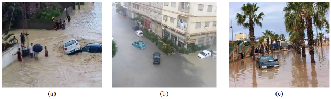
Figure 1 Pictures show the historic of flooding in the northern region in the last few years, (a) TTN on 1/03/2021, (b) TGR on 08/02/2021, and (c) LRC on 05/04/2022
According to local media, 275 residences were affected, and a huge number of vehicles were swept away by the water. The rainfall intensity recorded during the period of flood events was collected from various meteorological sites, providing insight into the amount of rainfall in these northern cities. At the TGR station, located at an elevation of 19 m, the highest precipitation intensities were recorded at 30 mm/h on February 25, 2021, and 28 mm/h on the exact date of the flood event, February 6, 2021. Meanwhile, at the Sania Ramel station in TTN, an intensity of 46 mm/h was recorded on the days experiencing flooding.
The main source of data was extracted from DEM provided by NASA’s Shuttle Radar Topography Mission (SRTM) and Landsat-8 imagery from 2016/01/01 into 2022/12/31. Based on the analysis of the different factors we have extracted the mean elevation recorded in each zone as illustrated in Table 1. The first step consists of extracting the numeric values of points from the eight raster using ArcGIS tools. As a result, the generation of the dataset including 10 columns split into the following manners: eight conditioning factors and the longitude and latitude position of each point.
Table 1 Dataset overview of three zones in Morocco: geographic, flood, and demographic factors
Area of
study
Number of rows Number of conditioning factors Area
(km2)
Mean
elevation (m)
Population
(habitant)*
TGR 186,620 8 169.58 71.56 1,060,261
TTN 102,206 90.120 43.56 547,177
LRC 23,689 22.28 22.35 495,030

Note: * is according to the High Commission for Planning in Morocco in 2014.

2.2 Methodology and methods

It is worth noting that, this study is one of the first research projects carried out in Morocco, especially since it covered three different regions with different characteristics. Research on flood prediction in Africa is relatively limited, comprising approximately 4.14% of the overall studies. Notably, Morocco stands out as a leading contributor with seven articles published on the subject between 2017 and 2022 (Antwi-Agyakwa et al., 2023), taking into account the contribution of applying and comparing for the first time different types of unsupervised learning to generate the map of flood prediction and mapping the topographic environmental variables based on remote sensing technology and GIS techniques. Figure 3 summarizes the methodology employed in this paper.
The first step is selecting the area of study based on a deep analysis of climatic, hydrologic, topographic, demographic, and historic floods in Morocco. Figure 1 provides images of flood damage in TGR, TTN, and LRC, captured on various dates from social media and local journals, illustrating severe impacts on infrastructure, streets, vehicles, and residential buildings. Figure 2, created using ArcGIS 10.4 software, depicts the geographical context of the northern region of Morocco, delineating the three study areas against a satellite background with insets highlighting high population density, the presence of buildings, and essential rivers. These figures collectively underscore the significance of the selected regions by illustrating the extent of flood damage and relevant geographical features. The next step is collecting data using the remote sensing technique, especially the Landsat-8 image and SRTM DEM applied on the platform Google Earth Engine (GEE) and ArcGIS software. Following that, we have explored nine conditioning factors related to surface topography and LU namely, elevation, slope, TPI, aspect, NDVI, LU, soil type, plan curvature, and profile curvature. These factors are visually represented in Figure 5, which maps the flood conditioning factors across the study areas. This map provides a detailed visualization of how each factor contributes to the flood susceptibility assessment. The main aim of this stage is to select the relevant factors to create the set of data needed to train the ML algorithms. At the stage of data pre-processing, we have employed two types of approaches to clean data and reduce the dataset. Therefore, two techniques were employed to clean the dataset, namely interquartile range (IQR), and feature scaling. As a result, the generation of three different datasets in terms of cell numbers but with the same attributes is known as flood conditioning factors. Taking into account the absence of historical data on flood events, it is essential to apply unsupervised ML models, especially K-means clustering and fuzzy logic methods to predict flood locations. The step of evaluating models comes next with the use of varied metric methods, in particular, the DBI and the silhouette coefficient score, finally generating the map of flood susceptibility.
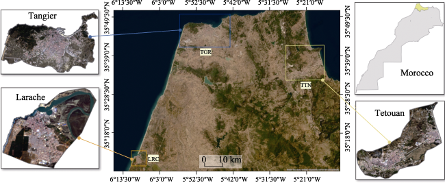
Figure 2 Detailed maps of study areas: three identified regions with square box boundaries in the WGS84- EPSG 4326 coordinate system
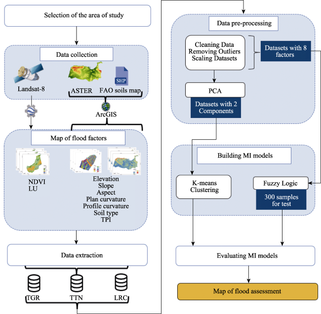
Figure 3 Flowchart of methodology for creating the flood susceptibility
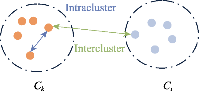
Figure 4 Description of clustering metrics
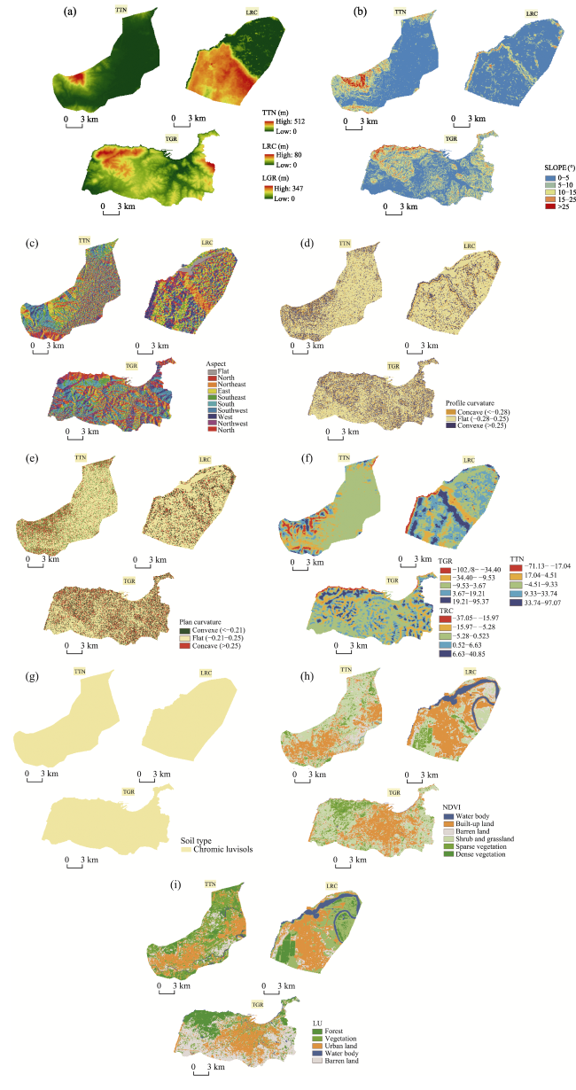
Figure 5 Maps of conditioning factors of the three zones (a. Elevation; b. Slope; c. Aspect; d. Profile curvature; e. Plan curvature; f. TPI; g. Soil type; h. NDVI; i. LU)
The step of generating flood conditioning factors was carried out with the aid of ArcGIS 10.4 software to extract factors from the SRTM DEM provided by the United States Geological Survey (USGS), Landsat-8 imagery from USGS, and soil type data sourced from the Food and Agriculture Organization (FAO) soils map. As for LU and NDVI, they were generated from Landsat-8 using an online platform GEE. This tool is defined as a cloud platform that helps upload large amounts of data, especially satellite imagery, over a long period, besides adding features and visualizing on a map the different methods used to extract factors with a generative legend (Safanelli et al., 2020). It is noteworthy that, remote sensing is the operation of observing, recording, and sensing an object or an event from a huge distance without any contact. The information is sent through electromagnetic waves. It is used to observe the earth, land, and atmosphere. The type of product produced by this technology is an image (Weng, 2010). Based on the scope, we have five categories of remote sensing namely satellite imagery, where the feature is taken from a satellite platform such as Landsat-8, photography or photogrammetry when the image is taken from a photograph to capture the visible light; thermal remote sensing, which uses the thermal infrared portion of the spectrum; radar imagery, when microwave wavelengths are used; and LIDAR technology, which is based on sending a laser pulse to the land and then calculating the time between the sending and reception of each pulse. On the other hand, it is vital to know that there are three types of interaction between radiation and Earth: the first is transmission, which represents the energy on the surface and depends on the wavelength; then we have reflectance, which is the amount of radiation reflected from the object to the source; and finally, emittance, which defines radiation absorbed by the object and then remitted, this happens mostly in the case of long wavelengths. The three types of radiation are used to calculate the Radiative Transfer Equation (RTE), which is a mathematical technique to describe the different interactions between the atmosphere and electromagnetic waves, and it is a primary step in taking satellite images. (Yu et al., 2014) This equation considers the radiance observed in a specific spectral band Bi in the following manners:
R i = T a × E i × L B i + 1 E i × I D i + I U i
where Ri represents the radiation received by a sensor in band i, Ta is the atmospheric transmission, Ei refers to the surface emissivity, L B iradian emitted by the target. IDi downwelling path radiance and IUi upwelling path radiance.
The selection of this particular software and technique combination was made by comparing raster results of conditioning factors obtained through both tools, while also considering insights from relevant literature. A consistent resolution was maintained, with all environmental variables having a fixed cell size of 30 meters, as described below:
Elevation is a primary factor that correlates inversely with floods regions with low elevation; are most likely to be affected by floods. Using SRTM DEM to extract the value of elevation, TGR recorded a high elevation of 347 meters above sea level, TTN reached a high elevation of 512 meters, and LRC has the lowest metric with a value of 80 meters. According to other related works, areas with high elevations are less susceptible to flood risk (Farhadi and Najafzadeh, 2021).
Slope is a physiographic setting with high impact, as it leads to the runoff of the water. A high slope value contributes to a high potential for flooding. This factor could be divided into five categories: 0°-5°, 5°-10°, 10°-15°, 15°-25°, and > 25° (Costache, 2019). In TGR, the maximum value of slope recorded is 49°, 44° in TTN, and 30° in LRC.
Aspect represents the highest slope in a defined direction, it is a crucial setting, as it precisely determines the flow direction of the slope. The raster of the result indicated, for each pixel, the direction in the range of 0 to 360 degrees. This indicator could be calculated with two methods: the geodesic algorithm and the planar way. In our case of study, we used the classic method of planer aspect calculation, which uses a window matrix of 3 rows and 3 columns from a , . . . , i to cover all pixels of the raster and calculate the value of the middle based on their eight neighbors. This algorithm calculates the value of the pixel in both directions of x and y in the following way:
d z d x   =     c   +   2 f + i × 4 w g h t 1     a + 2 d + g × 4 w g h t 2 8
d z d y   =     g + 2 h + i × 4 w g h t 3     a + 2 b + c × 4 w g h t 4 8
where wght1 and wght2 represent the horizontal weight number of valid cells.
After calculating the value in each horizontal and vertical direction of the cell target, we calculate the value of the Aspect using the following equation:
A s p e c t e   =   57.29578 × a t a n 2 d z d y , d z d x
The result should be converted into degree units considering three cases, namely:
A s p e c t < 0 : A s p e c t D e g r e e = 90 c e l l v a l u e
0 < A s p e c t < 90 : A s p e c t D e g r e e = 90 c e l l v a l u e
A s p e c t > 90 : A s p e c t D e g r e e = 360 c e l l v a l u e + 90
The raster result is classified into 10 classes divided in the following manner: -1°, 0°-22.5°, 22.5°-67.5°, 67.5°-112.5°, 112.5°-157.5°, 157.5°-202.5°, 202.5°-247.5°, 247.5°-292.5°, 292.5°-337.5°, 337.5°-360°, Flat, North, Northeast, East, Southeast, South, Southwest, West, Northwest and North, respectively.
Profile curvature represents the changes in slope value in each cell of a raster in the direction of dipping (Ayalew et al., 2004). This factor contributes to describing the surface if it is concave, horizontal, or convex, using three classes, respectively: <-0.28, -0.28 - 0.25, and >0.25.
Plan curvature represents the rate of the curve surface perpendicular to the slope surface and aims to control the entering and out of the flow of water on the slope. It is divided into three classes: convex, flat, and concave with interval values of <-0.21, -0.21 to 0.25, and > 0.25, respectively.
TPI reflects the difference in altitude between the current cell and its neighbor (Costache, 2019) and it is divided into five classes. The calculation process uses a window of 33 by 33 cell neighborhoods to generate the mean value of the center cell, then abstracting the result from the central elevation cell employing the following equation:
T P I i   =   E 0 n 1 E n n
where E0 is the elevation of the central cell, and n is the total number of neighbors cells.
If the TPI is near or equal to zero, indicates a flat surface, if the value of the cell is higher than its neighbor, named large positive, we have a ridge or a hill, and finally, if the value of the cell is lower than the surrounding areas, named large negative, indicates the occurrence of a valley or bottom (DeLancey et al., 2019).
Soil type has a crucial impact on floods, the high rate of soil infiltration leads to low runoff water, thus mitigating the risk of this natural hazard. In three regions, we have the same type of soil named LC (Chromic Luvisols) (Talukdar et al., 2020).
LU from a literature point of view has a crucial impact on flood occurrences (Tehrany et al., 2019). According to studies one of the important classes extracted is forest, and with the presence of a large surface of this type, we have a high chance of mitigating the runoff and avoiding flood damage. In this work, we have used Landsat-8 images to classify features into 5 classes: forest, vegetation, water body, urban land, and barren land, using the software ArcGIS 10.4. This classification procedure played a primary role in constructing a dataset, comprising 212 individual records, which formed the foundation of our analysis. Subsequently, we employed advanced ML models, specifically RF and Classification and Regression Tree (CART) algorithms. These models were used to discern and identify the land type for each cell in our raster dataset. To determine the model that would deliver the highest accuracy in correctly classifying LU, we randomly divided the dataset into 80% for training and 20% for testing. This rigorous assessment allowed us to select the RF algorithm, which exhibited the highest accuracy scores of 75%, 83%, and 80% in TGR, TTN, and LRC, respectively, for LU classification.
NDVI ranges between -1 and 1, and could be divided into six classes as follows: water body, built-up land, barren land, shrub and grassland, sparse vegetation, and dense vegetation, with range values of -0.28 to 0.015, 0.015-0.14, 0.14-0.18, 0.18-0.27, 0.27-0.36, and 0.36-0.74, respectively; NDVI is calculated based on both band red and near-infrared (NIR) reflected by vegetation, which corresponds to bands 4 and 5 in Landsat-8 imagery (Pettorelli et al., 2005):
N D V I   =   N I R     R E D N I R   +   R E D
By applying the vectorization technique function “Raster to Point”, we convert the raster maps representing the nine flood conditioning factors into a vector format consisting of points. In this transformation, each cell within the raster map was converted into an individual point. The value associated with each point corresponded to the value of the original cell, and the point position was determined by the center and summit of the respective cell. Table 2 provides a brief overview of the metadata associated with the environmental factor parameters:
Table 2 Descriptive overview of conditioning factor data sources
Conditioning factors Source of data GIS data type Time Resolution
Elevation DEM Grid - 30 m ×
30 m
Slope -
Aspect -
Plan curvature -
Profile curvature -
TPI -
LU Landsat-8 From 2016-01-01 into 2022-12-31
NDVI From 2016-01-01 into 2022-12-31
Soil type FAO soils map Vector - -
Before training ML models, it is crucial to ensure good quality data that generates a reliable result. Considering this fact, the stage of data pre-processing was composed of three steps which are usually the most common in the field of data preparation. Firstly, ensure that our dataset is clean of missing values, secondly, remove outliers (Dixon, 1953) which represent an error that could negatively impact the result of classifier methods. In this context, we have applied the IQR (Nair and Kashyap, 2019) method to detect the aberrant points. As a result, we have defined the first and third quartiles as Q1, and Q2, respectively. Then calculate the IQR using the following equation:
I Q R = Q 1 Q 2
The rate value reflects the mean distribution of data, helping to find lower and upper bounds. Using a scatter plot, we visualized each conditioning factor for the three regions, and with a good understanding of the data source, we successfully eliminated points outside the lower and upper bounds. The number of samples was changed from 25,268 to 23,689, from 102,689 to 102,206, and from 186,753 to 186,620 in zones LRC, TTN, and TGR, respectively. The second method of linear transformation allowed to beyond the value of conditioning factors between a range of 0 and 1 (Kumar Singh et al., 2015). Thus, contributes to avoiding the domination of samples with the highest value. The result is given by the following equation:
N C i = C i min C i max C i min C i
where Ci is the value of a conditioning factor of a cell index i.
The final step employs PCA, which is a statistical technique for feature extraction to reduce the dimension of the dataset, this method tries to find patterns in data with a lot of features (Yariyan et al., 2020) to feed it to the process of ML. It is a primordial tool to create a subspace containing vectors of maximum variance directions in the original dataset, where t represents the initial dimension of the vectors and f the new dimension of vector after applying the following equation (Martinez and Kak, 2001):
y i = L T x i, i   = 1 , . . . , N
where yi is the new feature vector, L is the linear transformation that reduces the dimension of the dataset form t to f.
Based on our deep understanding of the factors and the results of the PCA, we identify environmental attributes that have a substantial impact on flood occurrence, leading us to focus on them for our analysis to build the K-means clustering.
During the development phase of unsupervised ML models, we worked on implementing two models: K-means clustering and fuzzy logic methods. Our primary objective is to identify the most precise model to create the flood assessment map. The ML process is divided into various types. In general, there are three types commonly used namely supervised learning, unsupervised learning, and reinforcement learning. In the case of unsupervised learning, the training dataset does not contain labeled data, and the process needs only these inputs without knowing the target. This method is based on discovering data and finding the right patterns with the highest similarity to form a class. In particular, K-means clustering is considered the first portioned method used for this domain of research, and the fuzzy logic method (Maspo et al., 2020). Below is a brief description of the primary algorithm adopted:
K-means clustering algorithm is a crucial technique to structure a data set, and it is divided into two general types, namely probability model-based methods and non-parametric models. Furthermore, the first type considers the different data points as a mix of probabilities calculated based on prediction and maximization algorithms. The second method calculates similarity or dissimilarity, whereas the most widely adopted algorithm is a partitioned method, which defines the distance between a point and the cluster prototype. The K-means clustering method represents the most commonly used algorithm in the literature, especially for flood prediction, moreover, it is an unsupervised technique to generate different classes that regroup samples with similar features (Stoyanova, 2023).
This algorithm is based on minimizing the cost function, which illustrates the distance between each sample xi (i = 1, …, N) and the centroid of the k cluster. The cost function considers that points are in Euclidean space, and the results were given by minimizing the cost function J (Dicks and Wales, 2022):
J μ = i = 1 N j = 1 k a i j x i μ j 2
where μj, the assignment of variable a to a fixed center represents the geometric centroid of cluster k. x i μ j  represents the distance between data point xi and the cluster centroid   μ j.
a i j = 1 , i f x i j cluster e . i k = x i μ j 0 , otherwise
Note the fact that, K-means clustering gives a good result if the data samples were placed around their centroid.
Fuzzy-logic is a semi-quantitative method based on a mathematical model. The Mamdani fuzzy inference system is the most widely used method proposed by Ebrahim Mamdani in 1975 (Perera and Lahat, 2015). This process contains four primordial steps namely fuzzification, evaluation of the antecedent, creating rules of aggregation, and defuzzification. The first step aims to scale the data between 0 and 1 using membership functions (MFs). MFs take various forms such as triangles, trapezoids, and bell curves to represent the distribution of data, whereas the triangle is the most used shape to define MFs as it shows the highest performance compared to other forms. The value of membership is calculated using the following equation (Costache et al., 2022):
M= i , f M i , i ϵ R
where M refers to the Fuzzy set, i element of the universe defined by R, and represents the membership function. The next vital stage is creating rules, which needs a deep knowledge of conditioning factors and their impact to identify the flood level risk. Rules could be established using logic operations (AND, OR) to obtain the final result. Consequently, we combine the different outputs of fuzzy logic rules, then apply the sum or maximum method to get the percentage of flood hazard, and finally, the defuzzification step to fetch the normalized output employing the appropriate methods.
The parameters for each model are provided in Tables 3-5, offering a concise summary of the various parameters utilized for both models.
Table 3 Parameters description of each unsupervised model
ML models Set of parameters
K-means clustering Number of clusters: {TGR=3, TTN=5, LRC=5}, Random state:{32}, Max iteration: {500}
Fuzzy logic method Membership function: {Triangular}, Coefficient of membership: {Table 4}, fuzzy logic rules: {Table 5}, output names: {low, moderate, high}, output membership: {(0, 0, 50), (25, 50, 75), (50, 100, 100)}
Table 4 Membership coefficients for flood conditioning factors
Environmental variables Linguistic variables Coefficient
LRC TTN TGR
C1 C2 C3 C4 C5 C6 C7 C8 C9
Elevation Low 0 10 20 0 50 100 0 50 100
Moderate 19 35 50 50 250 450 50 150 200
High 49 65 85 400 550 600 198 340 340
Slope Low 0 10 15 0 10 15 0 10 20
High 15 20 30 15 20 38 20 30 43
LU Forest 1 1 2 1 1 2 1 1 2
Vegetation 1 2 3 1 2 3 1 2 3
Water body 2 3 4 2 3 4 2 3 4
Urban land 3 4 5 3 4 5 3 4 5
Barren land 4 5 5 4 5 5 4 5 5
Profile
curvature
Concave -2 -1.4 -0.28 -2 -1.4 -0.28 -4 -1.4 -0.28
Flat -0.8 0 0.8 -0.8 0 0.8 -0.8 0 0.8
Convex 0.28 1.4 2 0.28 1.4 3 0.28 1.4 4
Plan curvature Convex -5 -3.14 -0.21 -5 -3.14 -0.21 -3 -3 -0.21
Flat -1.12 0 1.12 -1.12 0 1.12 -1.12 0 1.12
Concave 0.21 3.14 5 0.21 3.14 3 0.21 2.14 4
TPI Valley -37 -1 0 -37 -1 0 -37 -1 0
Flat 0 1 7 0 1 11 0 1 11
Ridge-hill 6 20 40 6 50 99 10 50 97
NDVI Water body 1 1 2 1 1 2 1 1 2
Built-up land 1 2 3 1 2 3 1 2 3
Barren land 2 3 4 2 3 4 2 3 4
Shrub and grassland 3 4 5 3 4 5 3 4 5
Sparse vegetation 4 5 5 4 5 5 4 5 5
Dense vegetation 5 6 6 5 6 6 5 6 6
Table 5 Some fuzzy logic rule set
Rules Input variables Output
1 Elevation [‘low’] AND Slope [‘high’] Risk [‘high’]
- - -
4 (Elevation [‘low’] OR TPI [‘valley’]) & LU [‘water body’] Risk [‘high’]
- - -
10 Elevation [‘high’] AND LU [‘forest’] AND NDVI [‘dense-vegetation’] Risk [‘low’]
- - -
15 (Elevation [‘moderate’] OR Elevation [‘high’]) AND NDVI [‘built-up’] Risk [‘moderate’]
24 rules are created based on the eight conditioning factors, the relation between factors and level of risk was carried out using different literature points of view, besides a profound understanding of the subject.
When validating clustering models, metrics such as the Silhouette Index and DBI are crucial for assessing performance and accuracy. These metrics help evaluate how well the model has grouped data points into clusters and whether the number of clusters chosen is appropriate.
Davies-Bouldin Index aims to select compact and separated clusters (Bolshakova and Azuaje, 2003), as in the following equation:
D B D = 1 n i = 1 n max Δ C i Δ c k δ C i , c k
where C : C 1 C 2 C i C n, n is the number of clusters in D, Δ(Ci) represents the “Intracluster” distance between two points in the same cluster, and δ(Ci, ck) defines the “Intercluster” distance between both clusters Ci and Ck.
To calculate the values of those distances, we have 36 methods: six for Intercluster distance and three for Intracluster distance with different combinations between these indices. For the first distance, we have the single linkage that represents the near distance between two points in different clusters, the complete linkage refers to the distance between the most remote points in different clusters, the average linkage defines the mean distance between two points, the centroid linkage represents the distance relative to the center of clusters, the average linkage refers to the average distance between the two centers of different clusters, and Hausdorff metrics generate the maximum distance of a point in a cluster relative to the nearest one in other clusters. The second distance includes complete diameter, which defines the distance connecting the most remote points in the same cluster, average diameter represents the mean distance between all points in this cluster, and finally, centroid diameter refers to the double average relative to the distance between all points and the center of this cluster.
The equation DB contributes to identifying clearly if we have a good cluster. Consequently, when the value of DB decreases to 0, we have compact clusters with a large distance between samples.
Silhouette index is based on the calculation of three primary values, namely silhouette width s(i), cluster silhouette Sk, and Global silhouette value GSD (Bolshakova and Azuaje, 2003).
Silhouette width s(i): We have Ck (k = 1, …, n) cluster, n the number of clusters, the silhouette method tries firstly to determine the quality measurement called silhouette width of point i in cluster Ck, to know if the sample i is a member of this cluster Ck using the following equation:
s i = d i a i max d i , a i
where d(i) represents the minimum average distance between sample i and all other samples classified in another cluster except the current one, which means C j k = 1 , , n , j k . a(i) represents the average distance between sample i and all samples of the Ck cluster.
The result of s(i) is beyond the values -1 and 1. The case of s(i) near to one means a “well cluster”, the sample i is in the right class Ck. When s(i) is closest to zero, the point i could be in both clusters the Ck and Ck-1 or Ck+1. Finally, the case of s(i) closes to -1, the sample i is “misclassified” into this cluster.
The Silhouette index of each cluster reflects the heterogeneity of classes. The equation of Ck is defined as follows:
S k = 1 N i n s i
where N is the number of samples in Ck clusters.
Global silhouette value GSD, taking into consideration the dataset D as D C : C 1 C 2...... Ci Cn is the union of all partitions, and n is the number of clusters. This method is defined in the following manner:
G S D = 1 n k n S k
The result of the value of GSD leads to predicting the cluster number to initialize unsupervised algorithms by selecting the k of the maximum value of GSD.
In the fuzzy logic algorithm, we initially created three prediction classes: low, moderate, and high. Subsequently, we defined fundamental rules based on the relationships between factors. To validate these models, we employed two key metrics namely, the silhouette index score and DBI. The chosen model was transformed into a flood assessment map which was operating with ArcMap software to provide a powerful tool for taking precise measurements and effectively managing this natural hazard.

3 Result and discussion

Regarding literature, the process of selecting the primary conditioning factors takes on various dimensions, depending on the area of study and data availability (Yariyan et al., 2020). This involves identifying and extracting relevant environmental attributes that significantly impact flood susceptibility. We prioritize factors based on their relevance and substantial influence on the outcome, ensuring that the most impactful variables are included. The classification of these factors is carried out using established criteria and techniques to create comprehensive indexes. Once the factors are classified, we train our model using these data inputs, applying appropriate algorithms to generate a detailed map of flood susceptibility. This approach ensures that the resulting map accurately reflects the flood risks based on the analyzed conditioning factors.

3.1 Maps of flood conditioning factors

The following section presents a series of maps depicting nine critical flood conditioning factors for the designated study zones of TGR, TTN, and LRC. These maps are generated to provide a comprehensive spatial analysis of factors influencing flood risks in these regions. Each map illustrates specific variables that contribute to flood conditions. In TGR, the region predominantly features gentle slopes and low elevations, with higher elevations mainly found at the extremities. The LU is primarily urban and barren land, though some forested areas help mitigate flood risk. In TTN, the landscape is characterized by low elevations, with the highest areas located in the Dersa Mountains. Most of the region has gentle slopes, but steeper slopes in certain areas contribute to increased flood risk. The land is a mix of urban land, barren land, and water-covered zones. LRC also exhibits low elevations and gentle slopes, with moderate vegetation along streams. The area includes significant barren and urban lands as well.
Upon analyzing the slope distribution in TGR, 6% of areas exhibit a slope ranging between 15° and 49°. On the contrary, a significant 94 % of zones are characterized by a slope under 15°, indicating the occurrence of runoff surfaces. The lower value is concentrated in the coastal region and on the urban surface, while the high value of the slope is located in the extremity of the area of work. Approximately 79% of areas reach an elevation of less than 100 meters, and 21% reach a high level, especially in the upper zone of this area. The LU and NDVI assume a crucial role in reflecting the flood occurrence. Therefore, in TGR, 20% of the area is occupied by forest and vegetation, with the presence of a high elevation making this region at very low risk of flooding. On the other hand, urban and barren lands dominate with a rate of 27% and 33%, respectively.
Based on the elevation map in TTN, it is evident that the highest rates are concentrated in the Dersa Mountains, illustrated in red and comprising 14% of the area, whereas the river “Oued Martil” situated within the lower valley is surrounded by medium elevation, indicating the presence of a stream. These lower elevations dominate the study area, with a rate of 86%. Examining slope, we observe that the majority of area features are located on low slopes, especially near the stream, constituting 93% of the region. The high slope, accounting for 7% of the region’s terrain, makes it susceptible to the risk of flooding. The vulnerability becomes more apparent according to the NDVI and LU maps, urban and barren lands surround the areas adjacent to streams at a rate of 60%, while water body covers 20%, and another 20% is designated as forestation zones.
LRC is characterized by low elevations, which reach a maximum of 80 meters, and they are mostly located in the southern zone. Conversely, the lowest elevations are recorded in approximately the “LOUKUS” stream. Moreover, the majority of the area exhibits a lower slope, with 84% of the terrain having a degree less than 15° and around 16% of features ranging from 15° to 30°. The LU and NDVI maps have distinctly delimited the stream, covering a range of 20% of the area with the distribution of moderate to dense vegetation. However, it is noteworthy that barren and urban spaces dominate, constituting 33% and 27%, respectively, which is quite promising.
Analyzing flood factor maps represented in Figure 5, the three regions are at an exceedingly high risk of flooding, primarily because of low elevations, proximity to the stream, and the invasion of urban development. This distribution reflects the pressing need to address several approaches to mitigate the damage and protect human lives.

3.2 Results of training ML models

The process of model selection involves choosing between K-means clustering and the fuzzy logic method based on their suitability for the study’s objectives. During the data pre-processing phase, certain factors such as soil type and aspect were excluded from the final datasets. This decision was made following a thorough evaluation of the extracted factors and their relevance to the analysis. Specifically, soil type was removed because it was categorized similarly across three distinct zones, as illustrated in Figure 5g. This redundancy rendered the soil type data non-informative for distinguishing between different flood-prone areas. Additionally, a correlation analysis revealed that the aspect factor exhibited a weak correlation with other variables, suggesting that it did not contribute significantly to the understanding of flood susceptibility. As a result, both soil type and aspect were excluded from all three datasets. This distribution underscores the urgent need to develop flood susceptibility maps to implement various strategies for mitigating damage and protecting human lives.
The process of categorizing flood risk levels involved applying K-means clustering to two critical factors: elevation and LU, as determined through PCA. The PCA results highlighted these factors as significant in distinguishing between different flood risk levels, leading to their selection for the clustering process. In the TGR region, K-means clustering was used to define three distinct flood risk classes: low, moderate, and high. This classification was guided by the silhouette score index, a metric used to evaluate the quality of the clustering. The silhouette score of 0.66 indicated a relatively high degree of separation between the clusters, suggesting that the three defined classes were effective in distinguishing different levels of flood risk. Additionally, the DBI score of 0.55 supported the validity of the clustering by indicating a moderate level of intra-cluster similarity compared to inter-cluster dissimilarity. In contrast, for the TTN and LRC areas, the K-means clustering process resulted in five distinct flood risk classes: very low, low, moderate, high, and very high. This finer classification was chosen to capture a broader range of flood risk levels and provide a more nuanced understanding of risk distribution. The clustering efficiency was assessed using both DBI and silhouette scores. For TTN, the DBI score was 0.50 and the silhouette score was 0.70, reflecting a good separation between the risk classes and a reasonable degree of intra-cluster cohesion. For LRC, the DBI score of 0.58 and silhouette score of 0.62 indicated slightly less optimal clustering compared to TTN but still demonstrated a satisfactory level of class differentiation. The choice of categorizing flood risk into these specific levels and evaluating the clustering results through DBI and silhouette scores ensured that the flood risk classes accurately represent varying degrees of risk across the study regions. The summarized results, as presented in Table 6, illustrate the effectiveness of the K-means clustering approach in differentiating flood risk levels in both areas of TGR, and TTN.
Table 6 Summary of the assessment outcomes for K-means and fuzzy logic models in each area of study
Zone Model Categories DBI Silhouette score
TGR K-means clustering Low Moderate High 0.55 0.66
Fuzzy logic Low Moderate High 0.51 0.56
TTN K-means clustering Very low Low Moderate High Very high 0.50 0.70
Fuzzy logic Low Moderate High 0.46 0.47
LRC K-means clustering Very low Low Moderate High Very high 0.58 0.62
Fuzzy logic Low Moderate High 0.35 0.54
The second approach employed in the flood risk analysis utilized precise rules and variable membership to classify areas into three distinct flood risk categories: low, moderate, and high. This method relies on predefined criteria and membership functions to determine the risk level based on a set of variables as presented in Tables 4 and 5, offering a rule-based approach to flood risk classification. To evaluate the accuracy and effectiveness of this model, a subset of 300 samples was used for testing. In the TGR region, the application of this model yielded a DBI score of 0.51 and a Silhouette score of 0.56. The DBI score indi-cates moderate intra-cluster similarity relative to inter-cluster dissimilarity, suggesting a reasonable separation between the risk classes. The Silhouette score reflects a fair level of cohesion within clusters and separation between them, indicating that the risk classes are adequately defined. In the TTN region, the model achieved a DBI score of 0.46 and a Silhouette score of 0.47. These scores suggest that while there is a decent level of class differentiation, there is room for improvement in the clustering’s clarity and separation. The relatively lower scores compared to TGR imply that the rule-based classification may have faced challenges in achieving clear boundaries between risk levels in this region. In the LRC region, the model excelled in identifying the most dangerous areas, with a DBI score of 0.35 and a Silhouette score of 0.54. The lower DBI score indicates a stronger separation between risk classes and better-defined clusters, while the Silhouette score reflects a good level of cohesion and separation, highlighting the model’s effectiveness in distinguishing high-risk areas.
The summarized evaluation findings for each algorithm, including both the K-means clustering and the rule-based approach, are presented in Table 6. These results provide a comprehensive view of how each method performed in categorizing flood risk and highlight the strengths and limitations of each approach in different regions.
These graphs depicting the importance of flood conditioning factors highlight notable differences in the significance of various factors across the study regions, as illustrated in Figure 6 and Table 7. Elevation, NDVI, and slope emerge as particularly crucial factors in the ML clustering process for flood risk assessment. Their importance varies significantly across the regions. In the TGR region, elevation and slope account for 64% of the relative importance in determining flood risk. This underscores their role in shaping the flood susceptibility in this region. In TTN, these factors are even more critical, with a relative importance score of 74%, indicating a stronger influence on flood risk assessment. The highest importance is observed in LRC, where elevation and slope contribute to 88% of the model’s relative importance. This substantial variability suggests that these factors are highly influential in determining flood risk in coastal and varied topographical areas.
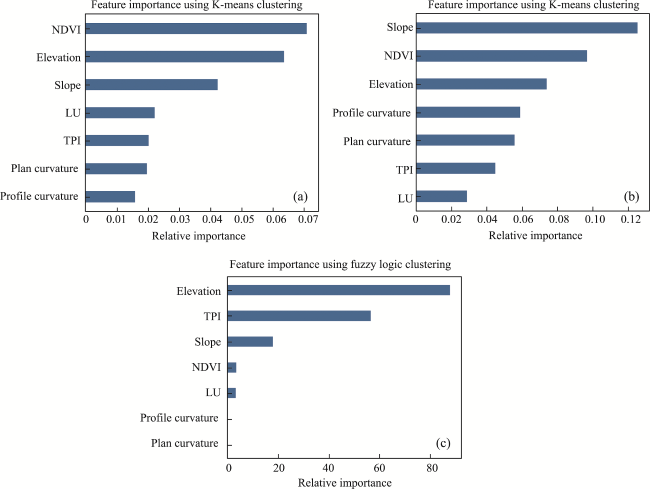
Figure 6 Flood conditioning factor importance using the best model (a. TGR; b. TTN; c. LRC)
Table 7 Relative importance values recorded using the best model
Features Relative importance (TGR) Relative importance (TTN) Relative importance (LRC)
Elevation 0.06 0.07 87.84
TPI 0.02 0.04 56.62
Slope 0.04 0.12 17.97
NDVI 0.07 0.09 3.50
Profile curvature 0.01 0.06 3.31
LU 0.02 0.03 0.14
Plan curvature 0.02 0.05 0.11
When using the fuzzy logic method in the LRC region, profile curvature and plan curvature are identified as having relatively low importance. This indicates that, in the context of LRC, these curvature factors do not significantly affect the flood risk classification compared to elevation and slope. The lower importance of these factors suggests that their contribution to determining flood susceptibility is limited, reflecting a regional specificity in the factors influencing flood risk. Overall, the variability in the importance scores across different regions highlights how flood risk factors can differ significantly depending on the geographical and topographical context. The higher significance of elevation and slope in certain regions points to their critical role in flood risk modeling, while the moderate influence of LU and NDVI and the lower importance of curvature factors in some areas provide insights into the relative contributions of various factors in different contexts.
Table 8 illustrates the distribution of flood risk levels across three zones: TGR, TTN, and LRC. In TGR, the area classified as low risk is 2678.31 ha, while the moderate risk area is the largest at 7585.03 ha, followed by a substantial high-risk area of 6485.43 ha. This indicates that TGR has a considerable portion of its region exposed to moderate and high flood risks. In contrast, TTN shows a diverse range of risk levels with a smaller very low-risk area of 307.48 ha and a modest low-risk area of 863.23 ha. The moderate risk area is significant at 3542.32 ha, and the high-risk area covers 1485.99 ha, with a large very high-risk area of 3005.82 ha, highlighting substantial flood risk across TTN. In LRC, the low-risk area is relatively small at 65.48 ha, while the moderate and high-risk areas are more prominent, covering 1038.07 ha and 994.48 ha, respectively. This distribution reflects LRC’s notable areas at moderate and high flood risk.
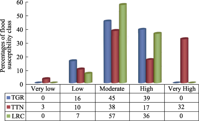
Table 8 Distribution of flood risk levels in TGR, TTN, and LRC
Zone Risk levels Area (ha)
TGR Low 2678.31
Moderate 7585.03
High 6485.43
TTN Very low 307.48
Low 863.23
Moderate 3542.32
High 1485.99
Very high 3005.82
LRC Low 65.48
Moderate 1038.07
High 994.48
The comparison of flood risk distributions across TGR, TTN, and LRC presented in Figure 7 reveals distinct risk profiles among these regions. TGR is predominantly characterized by moderate and high-risk areas. In contrast, TTN exhibits a more varied risk distribution, including a small percentage of very low-risk areas and a significant portion classified as very high-risk. This broad spectrum highlights TTN’s diverse flood risk environment, with a notable proportion of the region at very high risk. LRC, on the other hand, shows a focus on moderate to high-risk classifications. The high proportion of moderate risk and a substantial high-risk area suggest a more concentrated risk profile compared to TTN but similar to TGR. Overall, while TGR and LRC experience moderate to high flood risks, TTN displays a broader range of risk levels, including a significant very high-risk category, indicating a greater variability in flood risk across the regions.
Figure 7 Distribution percentages of flood risk level in TGR, TTN, and LRC
According to the findings from the DBI and the silhouette score, the most effective model for generating the flood risk assessment map for the TGR region is K-means clustering. The silhouette score of 0.66 indicates a good level of classification accuracy. Figure 8 illustrates three distinct flood risk classes: low, moderate, and high-risk flooding. A substantial portion of the TGR region, specifically 39%, is classified as high risk. These high-risk areas are primarily located in the central and eastern parts of the city, which are likely more vulnerable due to factors such as lower elevation, proximity to water bodies, and denser urban development. In contrast, 16% of the area falls into the low-risk category. These low-risk zones are situated in the western regions, characterized by higher elevation and dense vegetation, which likely provide natural barriers against flooding. The remaining 45% of the area is categorized as moderate risk. These areas are predominantly found in the southern parts of the region. The moderate-risk classification suggests a mix of factors that contribute to flooding, such as intermediate elevation and less dense vegetation compared to the low-risk areas.
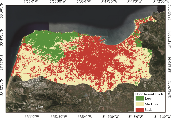
Figure 8 Map of flood hazard assessment in TGR using K-means clustering
Furthermore, the evaluation reveals that in the TTN region, K-means clustering is the most effective model for predicting flood risk, evidenced by a high silhouette score of 0.70, the highest among the evaluated regions. The flood risk distribution in TTN shows that 3% of the area is at very low risk, 10% is at low risk, and 38% is at moderate risk as demonstrated in Figure 9. Conversely, 17% of the area is classified as high-risk, and approximately 32% falls within the very high-risk category. These results indicate that the majority of TTN is at moderate to very high risk of flooding, necessitating immediate attention to flood prevention and mitigation measures in the high and very high-risk zones. The small portions classified under very low and low risk are likely in areas with favorable topographical features, such as higher elevation and better drainage systems.
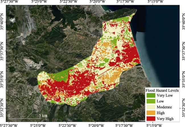
Figure 9 Map of flood hazard assessment in TTN using K-means clustering
In contrast, the LRC region demonstrates the effectiveness of the fuzzy logic method for flood risk assessment, evidenced by the best DBI value of 0.35, which indicates well-separated classes with minimal overlap. This underscores significant variations in flood risk distribution across the study area. Figure 10 highlights that LRC has 36% of its area classified as high risk, 57% as moderate risk, and only 7% as low risk. These findings suggest that the majority of LRC faces substantial flood risks, necessitating focused mitigation efforts for the high and moderate-risk areas. The clear delineation of risk categories provided by the fuzzy logic method enables precise targeting of flood prevention measures, thereby enhancing the overall resilience of the region to flooding events.
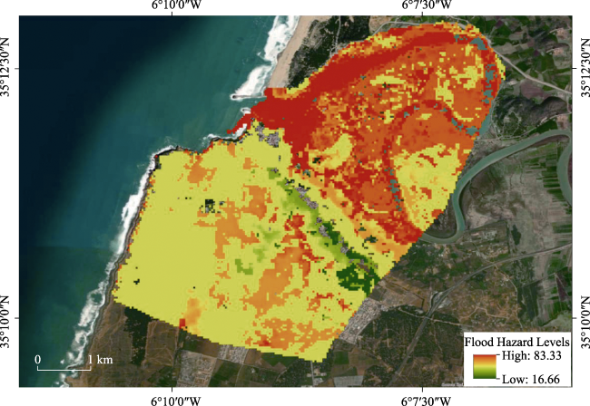
Figure 10 Map of flood hazard assessment in LRC using the fuzzy logic method
Figure 11 illustrates the distribution of flood factors based on the mean normalized risk level cluster in each region, providing a detailed insight into the underlying causes of flood risk variations. In the TGR region, the analysis reveals that high-risk levels are closely associated with low elevation and slope values. Conversely, low-risk levels are influenced by favorable LU types such as forests and vegetation, along with moderate to high elevations, which offer natural protection against flooding. In the TTN region, the highest flood risk is predominantly linked to low elevation and barren LU, emphasizing the vulnerability of these areas to flooding. Conversely, areas with high elevation and significant slope, as well as forested or vegetated LU, exhibit the lowest flood risk, mirroring the patterns observed in the TGR region. The LRC region presents a more complex scenario. Approximately 7% of the area is categorized as having a low risk of flooding due to high elevation and TPI values, even when water resources are present. However, areas near the "LOUKOUS" river, characterized by low elevations, are at significant risk of flooding. This highlights the crucial role of elevation and proximity to water bodies in determining flood risk.
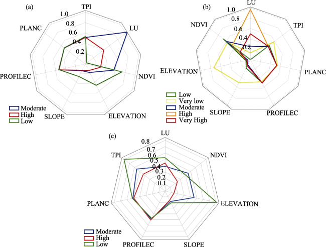
Figure 11 Mean Normalized index values of flood conditioning factors and the risk level identified in each region of study (a. TGR; b. TTN; c. LRC)

3.3 Discussion

The objective of this paper is to create an efficient and advanced solution for the proactive management of natural hazards, particularly floods. To achieve this goal, two robust techniques, inspired by GIS and AI, were applied to Landsat-8 imagery and DEM data to extract influential factors. The application of distinct unsupervised models, K-means clustering and the fuzzy logic algorithm, on three zones TGR, TTN, and LRC generate relevant results. The best model selected for both region TGR and TTN was K-means clustering with a good rate of silhouette score and DBI value, where fuzzy logic was the optimal model for LRC regions. The finding maps of prediction show that the high-risk level of the flood is concentrated in the region near the principal streams, for example along the rivers “LOUKOUS” and “Oued Martil” as well as in the coastal perimeters. It is worth mentioning that the DBI and silhouette scores generated over both areas of TGR and TTN zones achieved approximately the same value.
The assessment of models indicates a satisfactory outcome, as reflected in the final maps of flood hazards that accurately align with reality. Additionally, our results were compared with those of other relevant studies, further confirming the precision of our findings. This literature comparison of the findings was done in terms of the ML adopted to predict areas vulnerable to flooding, the accuracy level of these algorithms, the conditioning factors used to build models, and the type of data sources employed. The comparative analysis of studies emerges as a pivotal step in evaluating the effectiveness of models and showcasing their ability to predict flooding. In this regard, we conducted a comparison between the regions TGR and TTN and the findings of works (Bouramtane et al., 2021) and (Sellami et al., 2022). In a related study (Sellami et al., 2022), conducted in Tetouan corresponding to TTN in our case study, the use of supervised learning to predict flood hazard maps achieved a high accuracy of 0.99 using the RF model with the extraction of eight flood factors, namely, elevation, slope, aspect, LU/LC, SPI, plan curvature, profile curvature, TPI, and TWI. The result confirms that the center and eastern regions, particularly near “Oued Martil” face a high risk of flood, with percentages of 36% very high risk and 19% high danger of flood, 18% moderate risk, 12% low risk, and 15% very low level. Comparing to our results, the K-means clustering records the same number of classes, and five categories, with 3% for a very low risk and 10% of the area falling within a low risk of flooding, a moderate level represents only 38%, 17% of the area shows a high risk of flooding, and 32% reaches a very high risk. Based on that, we conclude that the k-means cluster approximately gives the same results as RF prediction, with minor differences due to the number of data points used and some differences related to the conditioning factors used. Although both works focus on flood risk assessment in the same city, TGR, there are notable differences in their classification. The study (Bouramtane et al., 2021) categorizes flood risk into four classes. It identified high and very high vulnerability areas in the center, east, southeast, and southwest, characterized by lowland terrain, and a high density of drainage channels. The CART model estimates that 19% of the total city area is in the highest proportion of very high-risk. In contrast, this paper applied K-means clustering, classifying the region TGR into low, moderate, and high-risk zones, with a significant portion of 39% falling into the high-risk category, primarily concentrated in the central and eastern parts of the city. While both studies highlight areas of high vulnerability, the differing methodologies, and classification approaches make direct comparisons challenging.
Table 9 Result of comparison between this paper and previous research
Related work Area of study The best model Accuracy Relevant factors Data source
(Talukdar et al., 2020) Teesta River basin, Bangladesh Bagging with the M5P
algorithm
AUC=0.945 LU/LC Landsat 8 DEM
Climatic data River map
(Meliho et al., 2022) Ourika,
Morocco
RF, XGB AUC=0.99 Rainfall and slope DEM
Inventory Map
(Bouramtane et al., 2021) Tangier, Morocco CART
SVM
AUC=0.99 Drainage density, Distance to rivers, and LU DEM
(Talha et al., 2019) Guelmim, Morocco FAHP - SMI, Rainfall, and Drainage density Landsat-8 OLI
DEM
(Sellami et al., 2022) Tetouan, Morocco RF AUC = 0.99 Elevation, Slope, Aspect, LU/LC, SPI, Plan curvature, Profile, Curvature, TPI, and TWI Sentinel 2B
DEM
(Parsian et al., 2021) Po-e Dokhtar and Nurabad, Iran AHP & fuzzy logic AUC=0.95 Distance to river, rainfall, and elevation Sentinel-1
DEM
(Xu et al., 2018) Haidian Island, China K-means
clustering
- Elevation, distance to rivers, and length drainage conduits Flood inundation model DEM
(Janizadeh et al., 2019) Tafresh Watershed, Iran ADT AUC=0.98 Lithology and Distance to the river Landsat OLI
DEM Local soil map
This work TGR K-means
clustering
DBI = 0.55
Silhouette Score = 0.66
Elevation, Slope, LU, and NDVI Landsat-8
DEM
TTN K-means
clustering
DBI = 0.50
Silhouette Score = 0.70
LRC Fuzzy logic DBI = 0.35
Silhouette Score = 0.54
The subsequent table presents a summary of the outcomes obtained from the comparison between this paper and related work:
Furthermore, the TGR and TTN regions exhibit clear associations between elevation, slope, and LU with flood risk, while the LRC region introduces additional complexity due to the significant impact of river proximity on flood risk. In the TGR region, flood risk is predominantly influenced by low elevation and gentle slopes, with natural LU features such as forests and vegetation providing effective flood mitigation. The TTN region mirrors these patterns but with a more pronounced impact from barren LU, exacerbating flood risk in low-lying areas by lacking natural flood barriers. In contrast, the LRC region’s flood risk profile is notably affected by proximity to the “LOUKOUS” river. Although high elevation and favorable topographic conditions typically reduce flood risk, areas near this river face significant risk due to low elevation and riverine influences. This highlights a critical aspect of flood risk management that is less prominent in the other regions: the direct impact of river systems on flood risk levels. While we acknowledge that river proximity can significantly impact flood occurrence, our study focuses on exploring the influence of topographic factors on flooding. By concentrating on variables such as elevation, slope, and LU, we provide a detailed analysis of how these elements contribute to flood risk across different regions. This approach allows us to isolate and understand the specific role of topography in flood dynamics, offering insights into how natural landforms and LU types affect flood risk independently of river influence. Focusing on topographic factors is crucial for understanding how water flows and accumulates in various landscapes for assessing flood risk. By analyzing these factors in detail, we can identify regions at risk due to their topographic characteristics, even in the absence of direct river influences.
Therefore, the key factors derived from the analysis of the three zones are elevation, LU, slope, and NDVI. Consequently, three distinct flooding risk scenarios emerge:
High risk: this scenario occurs when low elevations are observed in areas near rivers, on the outskirts of watersheds, or in regions with barren and built-up land, especially with the presence of water resources.
Moderate risk: is often associated with a correlation between high elevation and specific LU types such as water bodies or urban areas. Additionally, it can occur in regions with low elevations where forests are present, as vegetation helps absorb water and mitigate surface runoff.
Low risk: this is characterized by high elevations and steep slopes, coupled with sparse vegetation or forest cover. These conditions reduce the likelihood of flooding.
Indeed, floods have a significant impact on communities and infrastructure, but with a scientific approach, we can effectively control and mitigate their effects. Our primary solution involves a thorough analysis of topographic factors such as elevation and slope, which is the major solution and the core of our study. By recognizing the significant impact of topographic factors, we can implement slope stabilization methods such as terracing (Sitharam et al., 2019), retaining walls (Behling, 2020), and vegetation (Chen et al., 2021) to stabilize slopes and reduce runoff. Our analysis results in a map of flood-prone areas, enabling us to recommend elevated construction for buildings in these zones to mitigate flood impacts. Additionally, by understanding runoff direction through our land surface analysis, we suggest creating artificial channels and swales to guide excess water away from vulnerable areas into safe drainage zones. This approach mirrors the successful case study from Genoa (Faccini et al., 2015), where artificial channels were used to manage stormwater and mitigate flood risk. By strategically designing these channels to accommodate the natural flow patterns and local topography, we can enhance the efficiency of flood prevention efforts, reduce damage to infrastructure, and protect communities from future flood events. Our findings underscore the significant role of vegetation and forest cover in mitigating flood risk, as highlighted in the study (Bradshaw et al., 2007). The research emphasizes that deforestation exacerbates flood risks, reinforcing the importance of maintaining and promoting vegetative cover. By enhancing water infiltration and reducing surface runoff, especially in upstream areas. Therefore, integrating increased vegetative cover into our flood prevention strategies is crucial for both improving water management and protecting vulnerable areas from severe flooding.
One notable limitation of our study is the lack of a comprehensive inventory map of historical flood events. This absence restricts our ability to explore and compare more ML models, which could provide additional context and enhance the accuracy of our risk assessments. Additionally, the models employed, such as K-means clustering, have inherent limitations, including the need to predefine the number of clusters, which may not always align with natural variations in flood risk. To address these limitations, future work could benefit from enhanced data integration, such as incorporating higher resolution datasets and additional variables like real-time meteorological data. Employing advanced modeling techniques, including ML algorithms and dynamic modeling approaches, can improve classification accuracy and responsiveness to changing conditions.

4 Conclusion and perspectives

This paper proposes an effective solution to generate a map of flood hazard prediction in the northern region of Morocco with the selection of three substantial zones. This study was guided by the use of GIS and remote sensing techniques to extract the most relevant factors that lead to flash floods. To achieve this goal, two models were employed, namely K-means clustering and the fuzzy logic algorithm. Regarding the experimental result, both models show a satisfying result in correctly identifying areas vulnerable to this phenomenon. It was conducted that, the K-means cluster shows so far, the best model for mapping flood susceptibility for two zones TGR, and TTN with silhouette score values of 0.66 and 0.70. Fuzzy logic was the best model selected for the region RLC with a DBI score of 0.35. The three regions have a pressing need to be managed to face flooding, especially with the high rate of flood recorded as follows: 78% in zone LRC, 49% in TTN and 45% in TGR. Noting that the main causes of flood detected in this study are in general the low elevation associated with the near distance to stream and the lack of space vegetation that play a primordial role in absorbing water in contrast to the urban and barren land surface that increase the runoff water. The efficient advantage of this study is given by the ability to test the performance of each model on different areas of study and validate the final results according to that comparison. The result of the present research will be useful for authorities and different actors to proactively identify areas with high potential for flooding. In the end, reaching a reliable outcome based on combining GIS, remote sensing, and ML depends on the quality and precision of the data extracted and the enhancement of ML parameters. Thus, in the feature work, we will focus on comparing the results of flood prediction models based on different sources of data, exploring and improving the accuracy of flood factors, and improving ML accuracy.
[1]
Antwi-Agyakwa K T, Afenyo M K, Angnuureng D B, 2023. Know to predict, forecast to warn: A review of flood risk prediction tools. Water, 15: 427. https://doi.org/10.3390/w15030427.

[2]
Ayalew L, Yamagishi H, Ugawa N, 2004. Landslide susceptibility mapping using GIS-based weighted linear combination, the case in Tsugawa area of Agano River, Niigata Prefecture, Japan. Landslides, 1: 73-81. https://doi.org/10.1007/s10346-003-0006-9.

[3]
Balestra F, Del Vecchio M, Pirone D et al., 2022. Flood susceptibility mapping using a deep neural network model:The case study of southern Italy. In: EWaS5. Presented at the EWaS5, MDPI, p. 36. https://doi.org/10.3390/environsciproc2022021036.

[4]
Behling C W, 2020. Slope stability problems and solutions in the Red River Valley. In: Geo-Congress 2020. Presented at the Geo-Congress 2020, American Society of Civil Engineers, Minneapolis, Minnesota, pp. 838-850. https://doi.org/10.1061/9780784482810.087.

[5]
Bolshakova N, Azuaje F, 2003. Cluster validation techniques for genome expression data. Signal Processing, 83: 825-833. https://doi.org/10.1016/S0165-1684(02)00475-9.

[6]
Bouramtane T, Kacimi I, Bouramtane K et al., 2021. Multivariate analysis and machine learning approach for mapping the variability and vulnerability of urban flooding: The case of Tangier city, Morocco. Hydrology, 8: 182. https://doi.org/10.3390/hydrology8040182.

[7]
Bradshaw C J A, Sodhi N S, Peh K S-H et al., 2007. Global evidence that deforestation amplifies flood risk and severity in the developing world. Global Change Biology, 13: 2379-2395. https://doi.org/10.1111/j.1365-486.2007.01446.x.

[8]
Chen X W, Wong J T F, Wang J-J et al., 2021. Vetiver grass-microbe interactions for soil remediation. Critical Reviews in Environmental Science and Technology, 51: 897-938. https://doi.org/10.1080/10643389.2020. 1738193.

[9]
Costache R, 2019. Flash-Flood Potential assessment in the upper and middle sector of Prahova River catchment (Romania). A comparative approach between four hybrid models. Science of The Total Environment, 659: 1115-1134. https://doi.org/10.1016/j.scitotenv.2018.12.397.

DOI

[10]
Costache R, Arabameri A, Moayedi H et al., 2022. Flash-flood potential index estimation using fuzzy logic combined with deep learning neural network, naïve Bayes, XGBoost and classification and regression tree. Geocarto International, 37: 6780-6807. https://doi.org/10.1080/10106049.2021.1948109.

DOI

[11]
DeLancey E R, Kariyeva J, Bried J T et al., 2019. Large-scale probabilistic identification of boreal peatlands using Google Earth Engine, open-access satellite data, and machine learning. PLoS ONE, 14: e0218165. https://doi.org/10.1371/journal.pone.0218165.

[12]
Dicks L, Wales D J, 2022. Elucidating the solution structure of the K-means cost function using energy landscape theory. The Journal of Chemical Physics, 156: 054109. https://doi.org/10.1063/5.0078793.

[13]
Dixon W J, 1953. Processing data for outliers. Biometrics, 9: 74. https://doi.org/10.2307/3001634.

[14]
Faccini F, Luino F, Sacchini A et al., 2015. Geohydrological hazards and urban development in the Mediterranean area: An example from Genoa (Liguria, Italy). Natural Hazards and Earth System Sciences, 15: 2631-2652. https://doi.org/10.5194/nhess-15-2631-2015.

[15]
Farhadi H, Najafzadeh M, 2021. Flood risk mapping by remote sensing data and random forest technique. Water, 13: 3115. https://doi.org/10.3390/w13213115.

[16]
Janizadeh S, Avand M, Jaafari A et al., 2019. Prediction success of machine learning methods for flash flood susceptibility mapping in the Tafresh Watershed, Iran. Sustainability, 11: 5426. https://doi.org/10.3390/su11195426.

[17]
Kumar Singh B, Verma K, Thoke S A, 2015. Investigations on impact of feature normalization techniques on classifier&apos’s performance in breast tumor classification. IJCA, 116: 11-15. https://doi.org/10.5120/20443-2793.

[18]
Li G Y, Liu J H, Shao W W, 2023. Urban flood risk assessment under rapid urbanization in Zhengzhou city, China. Regional Sustainability, 4(3): 332-348.

DOI

[19]
Martinez A M, Kak A C, 2001. PCA versus LDA. IEEE Transactions on Pattern Analysis and Machine Intelligence, 23: 228-233. https://doi.org/10.1109/34.908974.

[20]
Maspo N-A, Bin Harun A N, Goto M et al., 2020. Evaluation of machine learning approach in flood prediction scenarios and its input parameters: A systematic review. IOP Conference Series: Earth and Environmental Science, 479: 012038. https://doi.org/10.1088/1755-1315/479/1/012038.

[21]
Meliho M, Khattabi A, Asinyo J, 2021. Spatial modeling of flood susceptibility using machine learning algorithms. Arabian Journal of Geosciences, 14: 2243. https://doi.org/10.1007/s12517-021-08610-1.

[22]
Meliho M, Khattabi A, Driss Z et al., 2022. Spatial prediction of flood-susceptible zones in the Ourika Watershed of Morocco using machine learning algorithms. ACI. https://doi.org/10.1108/ACI-09-2021-0264.

[23]
Mosavi A, Ozturk P, Chau K, 2018. Flood prediction using machine learning models: Literature review. Water, 10: 1536. https://doi.org/10.3390/w10111536.

[24]
Nair P, Kashyap I, 2019. Hybrid pre-processing technique for handling imbalanced data and detecting outliers for KNN Classifier. In: 2019 International Conference on Machine Learning, Big Data, Cloud and Parallel Computing (COMITCon). Presented at the 2019 International Conference on Machine Learning, Big Data, Cloud and Parallel Computing (COMITCon), IEEE, Faridabad, India, 460-464. https://doi.org/10.1109/COMITCon.2019.8862250.

[25]
Parsian S, Amani M, Moghimi A et al., 2021. Flood hazard mapping using fuzzy logic, analytical hierarchy process, and multi-source geospatial datasets. Remote Sensing, 13: 4761. https://doi.org/10.3390/rs13234761.

[26]
Perera E D P, Lahat L, 2015. Fuzzy logic based flood forecasting model for the Kelantan River basin, Malaysia. Journal of Hydro-environment Research, 9: 542-553. https://doi.org/10.1016/j.jher.2014.12.001.

[27]
Pettorelli N, Vik J O, Mysterud A et al., 2005. Using the satellite-derived NDVI to assess ecological responses to environmental change. Trends in Ecology & Evolution, 20: 503-510. https://doi.org/10.1016/j.tree.2005.05.011.

[28]
Rincón D, Khan U, Armenakis C, 2018. Flood risk mapping using GIS and multi-criteria analysis: A Greater Toronto area case study. Geosciences, 8: 275. https://doi.org/10.3390/geosciences8080275.

[29]
Safanelli J, Poppiel R, Ruiz L et al., 2020. Terrain analysis in Google Earth Engine: A method adapted for high-performance global-scale analysis. IJGI, 9: 400. https://doi.org/10.3390/ijgi9060400.

[30]
Sellami E M, Maanan M, Rhinane H, 2022. Performance of machine learning algorithms for mapping and forecasting of flash flood susceptibility in Tetouan, Morocco. The International Archives of the Photogrammetry, Remote Sensing and Spatial Information Sciences, XLVI-4/W3- 2021, 305-313. https://doi.org/10.5194/isprs-archives-XLVI-4-W3-2021-305-2022

[31]
Sitharam T G, Mantrala S, Verma A K, 2019. Analyses and design of the highly jointed slopes on the abutments of the world’s highest railway bridge across the Chenab River in Jammu and Kashmir State, India. In: Sundaram R, Shahu J T, Havanagi V (eds.). Geotechnics for Transportation Infrastructure, Lecture Notes in Civil Engineering. Singapore: Springer, 15-32. https://doi.org/10.1007/978-981-13-6713-7_2.

[32]
Stoyanova E, 2023. Remote sensing for flood inundation mapping using various processing methods with Sentinel-1 and Sentinel-2. The International Archives of the Photogrammetry, Remote Sensing and Spatial Information Sciences, XLVIII-M-1-2023,339-346. https://doi.org/10.5194/isprs-archives-XLVIII-M-1-2023-339-2023.

[33]
Talha S, Maanan M, Atika H et al., 2019. Prediction of flash flood susceptibility using fuzzy analytical hierarchy process (FAHP) algorithms and GIS: A study case of Guelmim region in southwestern of MOROCCO. The International Archives of the Photogrammetry, Remote Sensing and Spatial Information Sciences, XLII-4/W19, 407-414. https://doi.org/10.5194/isprs-archives-XLII-4-W19-407-2019.

[34]
Talukdar S, Ghose B, Shahfahad Salam R et al., 2020. Flood susceptibility modeling in Teesta River basin, Bangladesh using novel ensembles of bagging algorithms. Stoch Environ Res Risk Assess, 34: 2277-2300. https://doi.org/10.1007/s00477-020-01862-5.

[35]
Tehrany M S, Jones S, Shabani F, 2019. Identifying the essential flood conditioning factors for flood prone area mapping using machine learning techniques. CATENA, 175: 174-192. https://doi.org/10.1016/j.catena.2018.12.011.

[36]
Teixell A, Arboleya M, Julivert M et al., 2003. Tectonic shortening and topography in the central High Atlas (Morocco). Tectonics, 22: 2002TC001460. https://doi.org/10.1029/2002TC001460.

[37]
Thankappan J, Mary D R K, Yoon D J et al., 2023. Adaptive momentum-backpropagation algorithm for flood prediction and management in the internet of things. CMC, 77: 1053-1079. https://doi.org/10.32604/cmc.2023.038437.

[38]
Weng Q, 2010. Remote Sensing and GIS Integration:Theories, Methods, and Applications. New York: McGraw-Hill.

[39]
Xu H, Ma C, Lian J et al., 2018. Urban flooding risk assessment based on an integrated K-means cluster algorithm and improved entropy weight method in the region of Haikou, China. Journal of Hydrology, 563: 975-986. https://doi.org/10.1016/j.jhydrol.2018.06.060.

[40]
Xu W, Chen J, Zhang X J et al., 2022. A framework of integrating heterogeneous data sources for monthly streamflow prediction using a state-of-the-art deep learning model. Journal of Hydrology, 614: 128599. https://doi.org/10.1016/j.jhydrol.2022.128599.

[41]
Yariyan P, Janizadeh S, Van Phong T et al., 2020. Improvement of best first decision trees using bagging and dagging ensembles for flood probability mapping. Water Resources Management, 34: 3037-3053. https://doi.org/10.1007/s11269-020-02603-7.

[42]
Yu X, Guo X, Wu Z, 2014. Land surface temperature retrieval from Landsat 8 TIRS: Comparison between radiative transfer equation-based method, split window algorithm and single channel method. Remote Sensing, 6: 9829-9852. https://doi.org/10.3390/rs6109829.

Outlines

/