Research Articles

Is the special economic zone an effective policy tool for promoting polycentricity? Evidence from China

  • HUANG Daquan , 1 ,
  • WANG Yiran 2 ,
  • ZHENG Longfei , 1, *
Expand
  • 1. Beijing Key Laboratory of Environmental Remote Sensing and Digital City, Faculty of Geographical Science, Beijing Normal University, Beijing 100875, China
  • 2. College of Urban and Environmental Sciences, Peking University, Beijing 100871, China
* Zheng Longfei (1995-), Assistant Professor, specialized in economic geography and urban studies. E-mail:

Huang Daquan (1971-), Professor, specialized in spatial planning and urban development. E-mail:

Received date: 2024-01-28

  Accepted date: 2024-08-30

  Online published: 2025-01-16

Supported by

National Natural Science Foundation of China(42271262)

National Natural Science Foundation of China(42301185)

China Postdoctoral Science Foundation(2023M730284)

Fundamental Research Funds for the Central Universities(2022NTST17)

Abstract

The special economic zone (SEZ) is an important place-based policy adopted by the Chinese government to simulate regional and urban growth, and existing studies mainly focus on the impacts of SEZs on local economic outcomes and productivity. This paper establishes the linkage between SEZ and urban spatial structure based on time-series nighttime light images spanning 2000 to 2020 in China. Through a set of time-varying difference-in- differences (DID) regressions at the county level, we find that the introduction of national SEZs has a significant negative impact on monocentricity, while provincial SEZs need to operate for 7 years before they have a substantial impact on spatial structure. However, the average effect masks great heterogeneity with respect to the characteristics and geographic location of zones. SEZs characterized by higher research and development (R&D) intensity, larger scale, and longer establishment duration have more pronounced effects on spatial structure. Geographically, the effects peak when SEZs are 5-15 km away from existing centers, and the effects of SEZs are mainly observed in urban areas and top-tier cities.

Cite this article

HUANG Daquan , WANG Yiran , ZHENG Longfei . Is the special economic zone an effective policy tool for promoting polycentricity? Evidence from China[J]. Journal of Geographical Sciences, 2024 , 34(11) : 2166 -2192 . DOI: 10.1007/s11442-024-2288-x

1 Introduction

Spatial structure plays an important role in urban growth. As an important dimension of spatial structure, the relationship between mono-polycentricity and urban growth has long been a topic of interest for scholars and policy-makers (Anas et al., 1998; Chen et al., 2019). Urban spatial structure not only reflects the distribution pattern of human activities but also influences the functioning and development of cities. Theoretical and empirical evidence has shown that the urban spatial structure exerts a significant impact on social equality and economic and environmental performance (Arribas-Bel and Sanz-Gracia, 2014; Zhang et al., 2017; Zhao et al., 2017; Han et al., 2020; Nijman and Wei, 2020; Huang et al., 2021a). Therefore, understanding the changing patterns and driving forces of urban spatial structure is essential for urban spatial planning strategies and sustainable development (Münter and Volgmann, 2020).
There are three main categories of factors that contribute to the changes in urban spatial structure: natural environment, socioeconomic development level, and policies. The first two categories of factors are stable in the short term, and active intervention in the spatial structure can only be achieved through policies (Anas et al., 1998; Lee, 2007). Geographic conditions serve as the foundation of urban development, as the construction and expansion of cities are constrained by factors such as the availability of land for development and natural resource endowment (Dadashpoor et al., 2019; Fei and Zhao, 2019). Additionally, socioeconomic development significantly shapes urban structure (Salvati et al., 2018). However, geographical conditions are inherent and have become less influential in shaping urban development due to advancements in technology and improved socioeconomic conditions. On the other hand, a city’s economic outcome and demographic characteristics do not change significantly in the short term. Therefore, policies, as a proactive intervention, can play a crucial role in shaping the spatial forms of urban development.
Between the nexus of policy and urban spatial structure, place-based policy may play a prominent role (Zheng and Wu, 2024). As an important part of development policy, place-based policies, such as investment in transport infrastructure and special economic zones, have been pursued by numerous governments over the past several decades (Duranton and Venables, 2018; Lu et al., 2019). These policies are designed to foster development in specific areas and have the potential to influence the location of economic activities, thereby impacting urban spatial structure (Kline and Moretti, 2014). In recent decades, SEZs, as a typical place-based policy, have been widely adopted by the Chinese government and have significantly promoted urban spatial expansion and economic growth (Gu et al., 2017; Fei and Zhao, 2019; Lu et al., 2019). Since the late 1970s, the Chinese government invested more than 18,000 square kilometers of land and large amounts of funds to construct more than 552 national-level and 1991 provincial-level SEZs 1 .
Existing studies have extensively explored the effects of SEZs on local economic outcomes and technology spillovers. However, the role of SEZs in urban spatial structure remains unclear. The SEZ policy is a prominent development strategy designed to attract foreign and domestic investment, stimulate cooperation and innovation in a specific area, and foster economic growth (Lu et al., 2019). Although previous studies have demonstrated that SEZs could significantly attract investment, accelerate knowledge spillover and economic growth, and promote urban land growth (Wang, 2013; Zheng et al., 2016; Zheng et al., 2017; Wang et al., 2022), there is a lack of empirical evidence for quantifying the effects of SEZs on spatial distribution of economic activities within cities. To address this research gap, we construct panel data on monocentricity from 2000 to 2020 based on time-series nighttime light images and estimate the causal effects of the introduction of SEZs on urban spatial structure at the county level through a set of time-varying DID regressions. In summary, this study aims to answer two questions. The first is whether and to what extent the introduction of SEZs affects the spatial structure, and the second is what type and location of SEZs are effective policy tools for promoting polycentricity.
This paper makes three contributions to the literature. First, we comprehensively examine the causal impact of SEZs on urban spatial structure at the national scale in China, which fills the knowledge gap. This study establishes an empirical linkage between place-based policies and urban spatial structure. Second, a method for constructing long-term panel data on urban spatial structure based on nighttime light images and pixel-based algorithms is developed in this paper, and this method can be easily adopted in other studies. In this paper, we use nighttime light satellite imageries to measure the spatial structure of economic activities within a city, rather than the spatial distribution of population, employment, and land-use patterns. Finally, we demonstrate that the introduction of SEZs is an efficient policy tool for urban planners to promote polycentricity. This study provides strong empirical evidence to answer the question of which types of SEZs have a substantial impact on urban spatial structure. We document that the SEZ effects on spatial structure vary by the characteristics and geographic locations of zones, including the administrative level, age, spatial size, pillar industry, distance to the CBD, and local development level. These findings have strong policy implications for urban planning, and are helpful for governments in establishing policy toolboxes tailored to local conditions.
The remainder of the paper is organized as follows. The next section presents a comprehensive review of the literature and develops the hypotheses. Section 3 introduces the methodology for measuring spatial structure and the empirical strategy. Section 4 shows the baseline results and robustness checks. Section 5 investigates the heterogeneities. Finally, Section 6 concludes.

2 Theoretical framework and hypothesis development

2.1 Spatial structure and urban growth

The classical monocentric city model formulated by Alonso (1964) is the most influential depiction of urban form in the 20th century, based on the assumption that all production activities occur in the central business district (CBD). However, as cities continue to expand, the urban spatial structure is becoming increasingly complex. The evolution of most cities is characterized by transformation from monocentric urban form to polycentric patterns (Lee, 2007; Meijers and Burger, 2010). On the one hand, employment subcenters emerge with population expansion and technological advancement (Arribas-Bel and Sanz-Gracia, 2014). On the other hand, cities are highly diversified in many aspects, leading to the emergence of multiple centers that perform diverse economic and spatial functions in the city (Lee, 2007; Cao et al., 2016; Fang et al., 2023).
Polycentric structure facilitates urban growth by reducing agglomeration diseconomies and “borrowing” size among urban centers (Zhang et al., 2017). It is widely recognized that contemporary urban structures mostly exhibit complex and polycentric patterns, and transitioning from a monocentric to a polycentric structure is considered an effective approach to mitigate agglomeration diseconomies (Fujita et al., 1997). A polycentric urban structure is believed to be more resilient in fostering economic growth, and a positive correlation between a polycentric spatial pattern and economic performance has been found in numerous studies (Meijers and Burger, 2010; Zhang et al., 2017). This polycentric spatial pattern has increasingly become a favorite planning strategy among urban planners and geographers as it aligns with the developmental demands of cities.
Urban spatial structure is affected by both market and government forces. The entire process of the formation and evolution of urban spatial structure is a dynamic one, during which urban activities are allocated into urban form (Anas et al., 1998). The location of these urban activities is influenced by both market forces and state interventions. In response to rapid urbanization, scholars have launched discussions and arguments from two main perspectives. One is from the economic perspective, which believes that urban spatial structure transformation results from multiple socio-economic forces, such as economic development and population growth (Cheng and Masser, 2003; Du et al., 2014). Factors such as land markets and agglomeration diseconomies have compelled industries and economic activities to move toward suburban areas, thereby promoting suburbanization and the emergence of subcenters (Huang et al., 2021b). Thus, the driving forces for the evolution of urban spatial structure primarily come from industrialization and marketization. The institutional perspective, on the other hand, emphasizes the government’s role and behavior in shaping urban spatial structure (Wang and Luo, 2022; Zhou et al., 2024). In China, where land is owned by the state and collectives, the government plays an important role in urban development and spatial structure changes. Urban planning strategies can enhance the appeal of suburbs and promote the relocation of economic activities. At the same time, China has been emphasizing subcenter construction to promote polycentric evolution, particularly through the utilization of SEZs (Li, 2020). Research indicates that urban polycentric planning significantly promotes the emergence of sub-centers in China (Liu and Liu, 2018). Assessing the impact of such government policies on urban spatial structure holds significant importance for urban development.

2.2 The impacts of special economic zones on spatial structure

SEZs are regions with special economic privilege and have been used by many developing countries as a policy tool to promote industrialization and economic growth (Wang, 2013). The establishment of SEZs enables governments to experiment with and cultivate new policies on a small scale within a special economic regime. The early-stage SEZs proved successful in several countries, achieving their initial goals of attracting foreign direct investment (FDI) and stimulating exports (Schminke and Biesebroeck, 2013; Zeng, 2021). Recognizing the limitations of relying heavily on fiscal incentives without substantial ties to the local economy, many countries have shifted toward the contemporary concept of SEZs. These modern SEZs exhibit more extensive connections with the local economy, have multifunctional characteristics, and lean toward higher value-added service sectors. Such features have the potential to spur economic growth and generate employment opportunities, both directly and indirectly (Lu et al., 2023).
SEZs are generally located in the suburbs of cities where land is inexpensive and have the potential to emerge as new subcenters. The establishment of SEZs is a typical place-based policy aimed at building industrial clusters, increasing employment, and attracting FDI to stimulate economic growth in China (Alder et al., 2016; Lu et al., 2019). During the 1980s, 14 national SEZs were established on the periphery of Chinese coastal cities and emerged as both industrial spaces and isolated areas attached to central cities. As of 2018, there were more than 2500 SEZs in mainland China, and most SEZs came to dominate suburban areas as new subcenters. These SEZs are often equipped with a bundle of preferential policies, including tax deductions, discounted land-use fees, streamlined administrative approval processes for firm registration, increased FDI, significant autonomy in industrial policy, and other favorable incentives (Alder et al., 2016; Zheng et al., 2017). Moreover, most SEZs are established on the fringe of urban areas, serving as both industrial spaces at the urban‒rural fringe and isolated islands with connections to the central districts (Cheng et al., 2017). Consequently, the establishment of SEZs indicates that the government has chosen to foster subcenters by designating specific zones with improved infrastructure and a package of preferential policies. We hereby propose our first hypothesis:
Hypothesis I: The introduction of SEZs has a significant negative impact on urban monocentric structure.
The performance of SEZs varies widely. Some SEZs with high economic performance have emerged as new subcenters. However, there are also some low-performing SEZs that are not attractive enough to firms and gradually decline into “ghost towns”. The vast majority of these low-performing zones are provincial SEZs. In terms of administrative level, SEZs can be classified into national SEZs and provincial SEZs in China. Table 1 presents a comparison of national SEZs and provincial SEZs. First, national SEZs are established upon approval from the central government, the establishment of which can effectively reflect state-level regional development strategies. However, provincial SEZs are established upon approval from the respective provincial governments, and their establishments are often shaped by the policy intentions of provincial governments and the distribution of land resources (Chen et al., 2022). Provincial SEZs exhibiting commendable performance may be upgraded to national SEZs. And approximately half of the national zones are upgraded from well-performing provincial zones. Second, the sum of all incentives brought by a national SEZ is larger than that of a provincial SEZ in China 2 . Third, the average spatial size of national SEZs is approximately 10 square kilometers, whereas provincial SEZs typically cover an area of less than 6 square kilometers. In conclusion, national SEZs possess higher management authority, more attractive incentives, and larger areas than provincial SEZs. Therefore, the policy effects of national SEZs on urban spatial structure are expected to be stronger than those of provincial SEZs.
Table 1 A comparison of national and provincial special economic zones
National SEZs Provincial SEZs
Approval department Central government Provincial government
Policy objective Achieving sustained regional development and technology spillover Enhancing local GDP and promoting
industrial development
Preferential policy Direct tax reductions and fiscal subsidies Local tax refunds and fiscal incentives
Policy implementation capacity Under the unified guidance of the central government Local governments acting independently and pursuing their own approaches
Number (in 2018) 552 1991
In addition to administrative level, other characteristics of an SEZ, such as type, age, spatial size, and pillar industries, may also affect its performance (Lu et al., 2023). The literature documents that the impact of SEZs on local economic outcomes and human capital varies depending on the characteristics of zones, including type, age and administrative level (Wang, 2013; Alder et al., 2016; Lu et al., 2023). For example, old SEZs have a higher positive impact on local FDI and wages than young SEZs (Wang, 2013). The introduction of an SEZ significantly increases the local high school enrollment rate, but this effect varies by zone type. Technology-oriented zones have a positive impact on education, while export- oriented zones show a negative impact. In summary, our second hypothesis is as follows:
Hypothesis II: The impacts of SEZs on spatial structure vary with zone characteristics.
There is a large spatial disparity in the level of economic development within and among prefectures in China, and geographic location may also affect the performance of SEZs. In China, geographical location is closely related to the agglomeration economy and transportation accessibility, which determines the attractiveness of zones to firms (Chang and Zheng, 2022). Previous studies have demonstrated that the performance of SEZ policy varies significantly among regions with different levels of economic development (Zheng et al., 2016). Within prefectures, urban areas generally have higher population density and transportation accessibility than peripheral counties in China. Among prefectures, the firm stock and economic activity intensity in top-tier prefecture-level cities are higher than those in low-tier cities. To investigate the heterogeneity of SEZ effects within and among prefectures, we conduct an empirical analysis at the county level. The third hypothesis is as follows.
Hypothesis III: The impacts of SEZs on spatial structure vary with the geographic locations of zones.
Figure 1 summarizes the conceptual framework and research hypotheses of this paper.
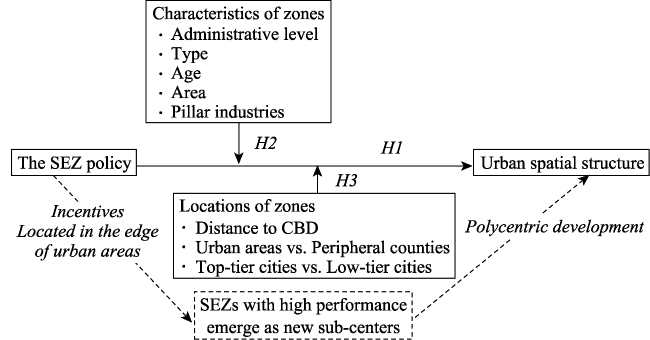
Figure 1 Conceptual framework

3 Empirical strategy and data statistics

3.1 Measurement of mono- and polycentricity

From the perspective of concentration, the degree of mono-polycentricity is often used to assess urban spatial structure in existing studies (Meijers, 2008) and is an important dimension of spatial structure (Li et al., 2022; Li and Du, 2022). Monocentricity reflects the extent to which economic activities are concentrated in urban centers (Li et al., 2018a).
Remote sensing images of nighttime light are excellent data for measuring urban spatial structure because they accurately predict the spatial distribution and intensity of economic activities (Long et al., 2018; Zheng et al., 2019). The indicators for measuring urban spatial structure are multifaceted, including factors such as the distribution of population, employment, and land-use patterns (Arribas-Bel and Sanz-Gracia, 2014; Wu et al., 2021). Concerning population and employment, a majority of studies utilize metrics such as population density and the spatial concentration of employment, often relying on census data or data tracking individual movements to represent urban spatial structure (Liu and Wang, 2016; Huang et al., 2017; Wu et al., 2021). Additionally, indicators such as land value (or rent) and morphological properties of built-up areas are commonly used to assess urban spatial structure (Wu and Yeh, 1999; Ding and Zhao, 2014). However, the availability and consistency of these aforementioned data are limited. As a result, existing studies usually quantify cross-sectional spatial structure at the prefecture level (Li et al., 2018b). For example, a demographic census at the subunit level within the county is conducted every ten years. The advent of remote sensing technology offers an opportunity to directly observe human activities. Long time series of remote sensing data, including nighttime light and impervious surface data, have become increasingly popular for measuring urban form (Cheng et al., 2017; Long et al., 2018).
In this paper, long-term nighttime light images 3 ), are adopted to calculate the degree of monocentricity at the county level. Following the literature (Chang and Zheng, 2022; Zheng et al., 2022), we combine adjacent urban districts into one observation unit called the urban area. First, county-level administrative boundaries are more consistent with the functional scope of cities than prefecture-level cities in China mainland (Ma and Long, 2020). Second, from the perspective of urban functions, a prefecture-level city usually includes a large central city (urban areas) and several peripheral small cities (peripheral counties) in China (Long, 2016; Ma and Long, 2020). The measurement of spatial structure at the prefecture-level leads to a significant underestimation of monocentricity. Finally, the number of county-level administrative units in China, rather than prefecture-level administrative units, is closer to the number of cities defined in the Global Human Settlement Layer Urban Centres Database (GHS-UCDB) 4 .
In this study, we focus on the spatial structure of economic activity distribution, rather on the population, employment, and land-use patterns. A number of existing studies have measured urban spatial structure from the perspective of mono-polycentricity (Hajrasouliha and Hamidi, 2017; Zhang et al., 2017; Li et al., 2018a; Li and Liu, 2018; Li and Derudder, 2022). Following the solid work of Li et al. (2020), our methodology for measuring monocentricity with nighttime lights includes three main steps: (1) identifying urban centers with high intensity of economic activities; (2) calculating the distance from each light pixel to the urban center; (3) measuring the degree to which economic activities in the entire city are concentrated in high-intensity areas.
In the first step, we identify the central business districts (CBDs) as the brightest cell in each county and urban area (Baum-Snow et al., 2017; Ch et al., 2021). We double check the location of identified CBDs, finding that the accuracy of the identification is 77.32%. We document that isolated outliers lead to false identification results. To address this issue, we classify pixels into four categories according to the values of local Moran’s I, and re-identify CBDs as the brightest cell from high-high (HH) category cells (Li et al., 2020). HH categories include cells with high light surrounded by those with high light. After manual double check, the accuracy of CBD identification reaches 96.03%. In the second step, we calculate the distance of each lit cell from the CBD and define the farthest distance between the lit cell from the CBD as the radius of city size.
In the last step, we use two indicators to reflect the degree of monocentricity of the urban spatial structure. Flowing the literature, the primary indicator (Mono_a) measures the inversed and weighted average distance of economic activities from the CBD by using the light luminosity of cell as the weight (Glaser and Kahn, 2001; Lee, 2007; Hajrasouliha and Hamidi, 2017), as follows:
$Mono\_{{a}_{j}}=\text{ }1-\underset{i=1}{\overset{n}{\mathop \sum }}\,\frac{{{e}_{i,j}}}{{{E}_{j}}}\times \frac{Dis\_CB{{D}_{i,j}}}{C{{R}_{j}}}$
where ei,j refers to the light luminosity of cell i in county/urban area j, and Ej is the total value of light luminosity in county/urban area j. n is the total number of cells in county/urban area j. Dis_CBDi,j represents the distance from cell i to the CBD, and CRj is the radius of county/urban area j. It appears that the high values of Mono_a correspond to the high degree of monocentric spatial structure.
The second indicator (Mono_b) of spatial structure measures the degree of agglomeration of economic activities into high-intensity CBD (Lee and Rodríguez-Pose, 2013; Achten and Lessmann, 2020). Specifically, we sort the cells in a county/urban area according to the intensity of economic activity (light luminosity), and calculate the proportion of cells with high luminosity relative to cells with low luminosity. The Mono_b index is specified as follows:
$Mono\_{{b}_{j}}=\underset{i=1}{\overset{n}{\mathop \sum }}\,{{E}_{i,j}}{{A}_{i-1,j}}-\underset{i=1}{\overset{n}{\mathop \sum }}\,{{E}_{i-1,j}}{{A}_{i,j}}$
where Ei,j is the cumulative proportion of nighttime light value in cell i, sorted according to the light luminosity in county/urban area j. Ai,j refers to the cumulative proportion of land area in cell i of county/urban area j. n is the total number of cells in county/urban area j. A low value of Mono_b corresponds to a low proportion of economic activities concentrated in the CBD area. In other words, a high value of Mono_b is high correlation with a great degree of monocentricity, which indicates that there are more economic activities concentrated in areas with high intensity of economic activities. It is worth noting that Mono_b does not incorporate the distance from the main center. However, it measures how far the actual distribution of human activities deviates from the equal dispersion, which can represent the degree of spatial concentration and, to some extent, the degree of monocentricity (Gordon et al., 1986; Small and Song, 1994). Therefore, Mono_b serves as a robust check for monocentricity in this paper.
Compared with the second indicator, the primary indicator Mono_a could better reflect the degree of monocentric structure of economic activities within a city. Because the primary indicator captures the influences of both the intensity of economic activities for each cell and its distance from the urban center. It is important to note that in Equations (1) and (2), the values of Mono_a and Mono_b have been normalized between 0 and 1 to facilitate comparison among counties/urban areas with different sizes.
Figure 2 presents the spatial distribution of nighttime light in four counties, accompanied by the corresponding indices of monocentricity. It can be clearly seen that Kunshan and Bazhou (Figures 2a and 2b), with relatively low values of monocentricity, do not have an obviously dominant urban center. In contrast, economic activities are highly centralized in high-intensity CBD in Yiwu and Mingguang (Figures 2c and 2d). The results highlight the efficacy of nighttime light data and these two indicators as accurate measures of urban spatial structure.
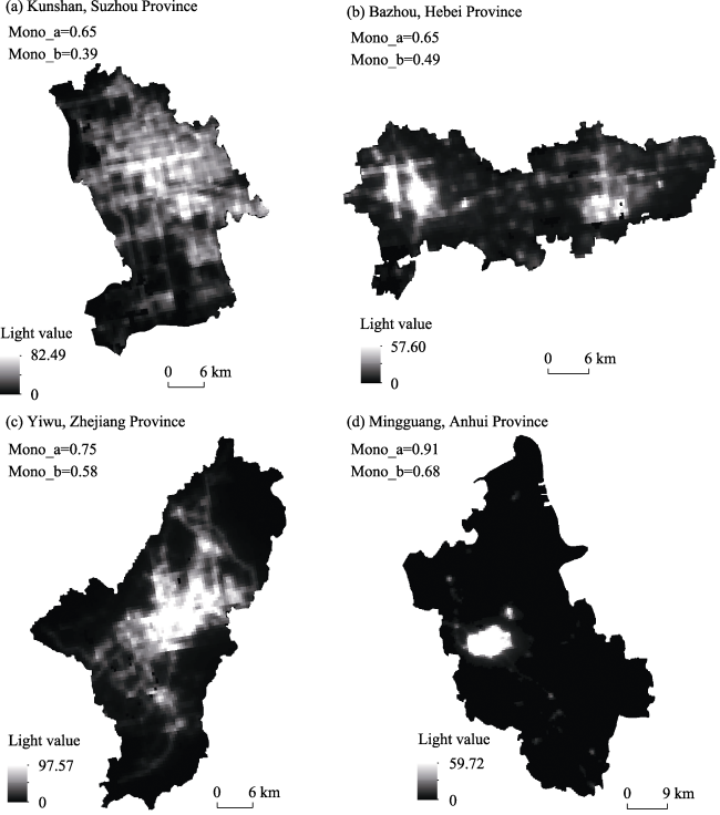
Figure 2 The nighttime light images of four county-level units

3.2 Empirical strategy

To explore whether and which types of SEZs affect urban spatial structure, our research includes two steps. First, we estimate the causal effect of SEZ introduction on spatial structure, which uses the time-varying difference-in-differences (DID) approach to help understand the average effect of SEZs on monocentricity. Next, we investigate which types of SEZs can have a significant impact on urban spatial structure through including interactions into DID regressions and subgroup analysis.
In this paper, a time-varying DID estimation from 2000 to 2020 at the county level is conducted to evaluate the effects of SEZs on urban spatial structure. The introduction of an SEZ can be regarded as a quasi-natural experiment for counties because the location choice of an SEZ is decided by the central and provincial governments, which is independent of local government influence. Following the literature (Chang et al., 2021; Zheng and Pan, 2024), we employ a time-varying DID model with two-way fixed effects to identify the policy effects of SEZs on urban spatial structure. Specifically, we control for county and province-by-year fixed effects to mitigate discrepancies in confounding variables between the treated and control groups. The DID model is formulated as:
${{Y}_{it}}={{\beta }_{0}}+{{\beta }_{1}}Time\times Treat+\mathop{\sum }^{}{{\beta }_{x}}\times Contro{{l}_{it}}+{{\mu }_{i}}+{{\tau }_{pt}}+{{\varepsilon }_{it}}$
where the dependent variable Yit is the degree of monocentricity of the urban spatial structure of county i in year t, which is measured by nighttime light and the indicators of Mono_a and Mono_b. The term Time×Treat represents the interaction term of the year dummy variable and binary policy variable. It is a time-varying dummy that equals one if a county introduces an SEZ after year t. Controlit is a vector of time-varying control variables measuring socioeconomic factors and natural environmental conditions of county i in year t, including economic outcome, population, industrial structure, annual average temperature, wind, humidity, and precipitation. μi represents the county fixed effect, and τpt represents the province-by-year fixed effect 5 . εit is random error.
The SEZ data are sourced from the National Development and Reform Commission of China (NDRC), which published the list of SEZs in 2006 and 2018, including information on type, name, administrative level, year of establishment, area, and pillar industries. Furthermore, on the basis of the pillar industries of each SEZ, we categorized the manufacturing SEZs into four groups (medium-low, medium, medium-high, high) using the OECD Taxonomy of Economic Activities Based on research and development (R&D) Intensity as a guiding framework. The longitude and latitude information of SEZs are extracted using a Python web crawler program from Gaode map (https://www.amap.com/). The socioeconomic data at the county level are collected from the China County Statistical Yearbook. And time-varying temperature, precipitation, wind, and humidity are obtained from the Resource and Environment Science and Data Center (RESDC) and the NASA Socioeconomic Data and Applications Center (SEDAC). Finally, we obtain panel data for 2167 county-level units in China from 2000 to 2020. Table 2 shows the descriptive statistical analysis of the variables.
Table 2 Variable definitions and summary statistics
Variable Description Mean SD Min Max
Panel A: Dependent variables
Mono_a Monocentricity is measured by adjusted and weighted
distance from the CBD.
0.76 0.16 0.01 0.99
Mono_b Monocentricity is measured by the degree of agglomeration of economic activities into high-intensity CBD. 0.43 0.12 0.05 0.81
Panel B: Independent variables
SEZ Time-varying dummy, 1 for counties/urban areas
with SEZ, 0 otherwise.
0.48 0.50 0.00 1.00
National SEZ Time-varying dummy, 1 for counties/urban areas
with national-level SEZ, 0 otherwise.
0.08 0.27 0.00 1.00
Provincial SEZ Time-varying dummy, 1 for counties/urban areas
with provincial-level SEZ, 0 otherwise.
0.45 0.50 0.00 1.00
Panel C: Time-varying control variables
GDP Gross Domestic Product (billion yuan) 22.12 97.86 0.03 3870.10
Pop Number of residents (thousand) 578.40 814.38 2.70 24650.00
Share of Secondary The share of add value in the secondary sector to GDP (%) 40.53 15.89 0.32 93.87
Share of Service The share of add value in the service sector to GDP (%) 36.79 11.40 1.08 93.90
Precipitation Annual average precipitation (cm) 94.29 44.75 2.29 338.92
Temperature Annual average temperature (℃) 16.14 5.23 -27.5 31.91
Wind Annual average wind speed (m/s) 2.06 0.63 0.52 6.77
Humidity Annual average relative humidity (%) 68.04 13.17 33.17 87.37

Notes: The dataset comprises 45,507 observations, encompassing a total of 2167 county-level units. Within this dataset, there are 285 urban areas and 1882 peripheral counties.

3.3 Stylized facts

Before the empirical examination is discussed, Figure 3 shows the stylized facts on the relationship between the spatial expansion of SEZs and urban spatial structure from 2000 to 2020. Figure 3a shows the distribution of national and provincial SEZs in 2000, and Figure 3c presents the changes in spatial structure during 2000-2010. The development of SEZs in China shows a pattern of expansion from coastal to inland areas. In 2000, the SEZs, especially the national SEZs, were primarily concentrated in coastal areas and the vicinity of provincial capitals, as mapped in Figure 3a). In 2009, the national strategy for upgrading provincial SEZs was launched, leading to approximately 300 provincial SEZs being elevated to the status of national SEZs. From 2000 to 2020, there was a substantial increase in the number of national SEZs (Figures 3a and 3b).
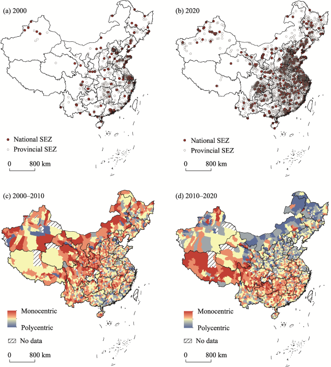
Figure 3 Distribution of special economic zones (a-b) and change in spatial structure in China at the county level (c-d) in 2000-2020
Comparing the spatial pattern of changes in SEZs and urban spatial structure, we find that the developing northern regions and developed southeastern coastal regions are developing toward a polycentric trend, especially the metropolitan areas where national SEZs are concentrated. This pattern suggests that the introduction of SEZs is likely to influence the urban spatial structure. The next section explores the causal effect of SEZs on spatial structure using regression analysis.

4 Baseline results

4.1 Baseline estimations

Table 3 reports the DID baseline results from employing Equation (3), and the standard errors in all regressions are clustered at the county level. Column (1) show the estimate of the average effect of SEZs on urban spatial structure. After controlling for time-varying control variables on socioeconomic factors and natural conditions, we find that the regression coefficient of SEZ on urban spatial structure is not statistically significant. In Columns (2), we separate the impacts of national and provincial SEZs by adding two time-varying dummies to Equation (3). The highly similar coefficients of SEZ between Columns (2) and (3) confirm that control variables, such as socioeconomic conditions, do not bias the DID estimations in this study. On the other hand, the results indicate that the introduction of national SEZs significantly reduces the degree of monocentricity, which is significant at the 1% level.
Table 3 Baseline difference-in-differences regression results
Mono_a Mono_b
(1) (2) (3) (4) (5) (6)
SEZ 0.005 0.003
(0.005) (0.002)
National SEZ -0.043*** -0.037*** -0.027*** -0.022***
(0.007) (0.007) (0.005) (0.004)
Provincial SEZ 0.005 0.004 0.003 0.0006
(0.005) (0.005) (0.002) (0.002)
ln (GDP) -0.035*** -0.033*** 0.011** 0.012**
(0.0082) (0.008) (0.005) (0.005)
ln (Pop) 0.015* 0.019** -0.031*** -0.029***
(0.009) (0.009) (0.005) (0.005)
Share of Secondary 0.16*** 0.153*** 0.139*** 0.134***
(0.037) (0.036) (0.022) (0.021)
Share of Service 0.16*** 0.156*** 0.1*** 0.092***
(0.036) (0.035) (0.021) (0.02)
ln(Precipitation) 0.004 0.004 -0.005 -0.004
(0.0085) (0.009) (0.005) (0.005)
ln(Temperature) 0.023 0.032 0.003 0.007
(0.3) (0.3) (0.157) (0.158)
ln(Wind) -0.018 -0.018 0.012* 0.012*
(0.012) (0.012) (0.006) (0.006)
ln(Humidity) -0.067 -0.066 -0.019 -0.018
(0.061) (0.061) (0.035) (0.035)
County fixed effects Yes Yes Yes Yes Yes Yes
Province-by-year fixed effects Yes Yes Yes Yes Yes Yes
Number of counties 2163 2164 2163 2163 2164 2164
R2 0.624 0.623 0.625 0.741 0.736 0.74
Observation 45,199 45,444 45,199 45,199 45,444 45,221

Notes: The standard errors are in parentheses and clustered at the county level. *, **, and *** denote significance levels of 10%, 5%, and 1%, respectively.

In contrast, the establishment of provincial SEZs does not have a significant impact on urban spatial structure. More importantly, the coefficients for national and provincial SEZ in Columns (2) and (3) are strikingly similar. This confirms that the county and province- by-year fixed effects capture unobservable factors well, and time-varying control variables has little impacts on the regression results. In the last three columns of Table 3, we replace Mono_a with Mono_b as the dependent variables in the regressions. The significance and sign of coefficients on monocentricity remain unchanged compared with those in the first three columns. Our baseline findings confirm that Hypothesis I holds for national SEZs, consistent with numerous studies indicating that national SEZs significantly impact regional development (Lu et al., 2023; Wang, 2013). However, it is noteworthy that provincial SEZs show non-significant effects, prompting us to further conduct heterogeneity analysis.

4.2 Tests on parallel trends assumption

The prerequisite of a valid DID estimation is the hold of the pretreatment parallel trends assumption. Following the literature, we input data in a standard event study frame to verify this assumption (Qin, 2017; Chang and Zheng, 2022). Specifically, we generate a set of lead- and lag-year indicators of actual SEZ operation to test the dynamic effects of SEZs. The model is specified as:
${{Y}_{it}}={{\beta }_{0}}+\underset{j=-6}{\overset{12}{\mathop \sum }}\,{{\delta }_{j}}SE{{Z}_{i}}\times 1\left[ j=T \right]+\mathop{\sum }^{}{{\beta }_{x}}\times Contro{{l}_{it}}+{{\mu }_{i}}+{{\tau }_{pt}}+{{\varepsilon }_{it}}$
where 1[j=T] is an event-time dummy variable for each lead and lag year before and after SEZ operation. The year prior to the SEZ (j=-1) is omitted and used as a reference year. The coefficients (δj) in other years indicate the effect of SEZs on the urban spatial structure relative to the reference year. All other variables are the same as those in Equation (3).
Figure 4 plots the coefficients with corresponding 99% confidence intervals from employing Mono_a as the dependent variable, which illustrates three key points. Firstly, the coefficients in the leading years (-6 to -2) are not significantly different from zero. This confirms that the parallel trend assumption is valid in the pretreatment periods. Secondly, the results of Figure 4 also provide evidence for the temporal trends of SEZ effects. The trends gradually turn downward after the operation of SEZs. This pattern suggests that counties/urban areas are moving toward a polycentric structure after the establishment of SEZs and that the magnitude of SEZ effects increases with age.
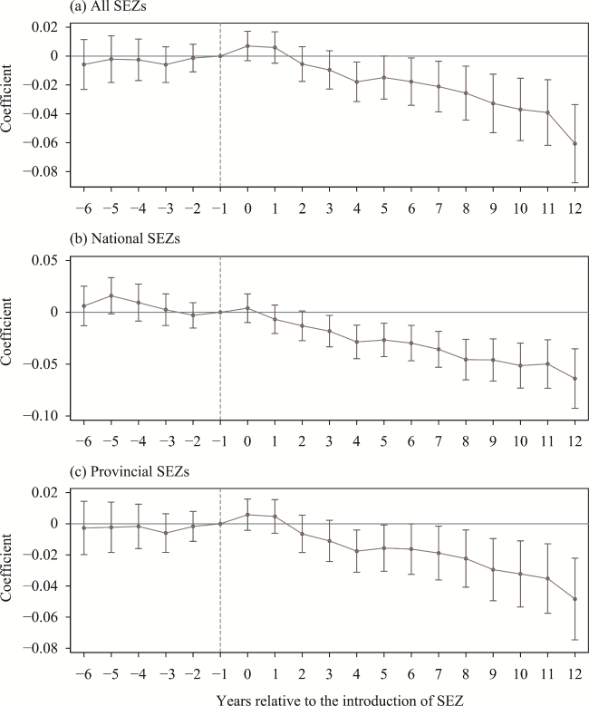
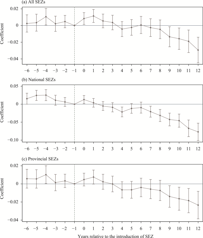
Figure 4 Event study of all special economic zones (a), national special economic zones (b) and provincial special economic zones (c)

Notes: 0 means the year when the first SEZ was launched, -1 represents the one year before SEZ operation and so on, and 1 refers to the time that is one year after SEZ operation.

Lastly but most importantly, compared with national SEZs, the introduction of provincial SEZs takes more years to have a significant impact on the local spatial structure. Figure 4b shows that a national zone has a significant influence on the spatial structure three years after its establishment. However, a provincial zone needs to operate for seven years to have a substantial impact on spatial structure, as evidenced in Figure 4c. As discussed in Section 2, approximately half of the national zones are upgraded from well-performing provincial zones. Consequently, the average age of national SEZs was 6.7 years higher than the provincial zones in 2016.
To check the robustness of our findings, we repeat the event study in Equation (4) using the Mono_b as the dependent variable. And the results are shown in Figure A1 in Appendix A, which are highly consistent with the findings in Figure 4. In summary, these findings in Figures 4 and A1 both confirm the validity of the pretreatment parallel trend assumption and well explain the diverse impacts between national and provincial SEZs in Table 3.

4.3 Robustness checks

The baseline results demonstrate that the introduction of national SEZs has a significant negative impact on monocentricity. However, whether the impact is affected by biases in the sample selection or identification strategy, must be addressed.
In this paper, the robustness check is based on the four strategies. The results of robustness checks are summarized in Table 4, which is organized by two panels. Panels A and B show the results with Mono_a and Mono_b as dependent variables, respectively.
Table 4 Robustness test results
Dropping metropolises Dropping the samples with more than one SEZ PSM-DID
(1) (2) (3) (4) (5) (6)
Panel A: Mono_a
SEZ 0.006 0.004 0.007
(0.005) (0.005) (0.005)
National SEZ -0.038*** -0.033*** -0.039***
(0.007) (0.011) (0.008)
Provincial SEZ 0.005 0.006 0.007
(0.005) (0.005) (0.005)
R2 0.625 0.626 0.629 0.629 0.568 0.569
Panel B: Mono_b
SEZ 0.002 -0.0009 0.001
(0.003) (0.003) (0.003)
National SEZ -0.024*** -0.015** -0.022***
(0.005) (0.007) (0.005)
Provincial SEZ 0.0002 -0.0001 0.001
(0.002) (0.003) (0.003)
R2 0.741 0.742 0.734 0.734 0.705 0.706
Number counties 2090 2090 2091 2093 1933 1933
Observations 43,680 43,680 40,539 40,539 40,379 40,379
Controls Yes Yes Yes Yes Yes Yes
County fixed effects Yes Yes Yes Yes Yes Yes
Province-by-year fixed effects Yes Yes Yes Yes Yes Yes

Notes: The standard errors are in parentheses and clustered at the county level. *, **, and *** denote significance levels of 10%, 5%, and 1%, respectively. The control variables are the same as those in Equation (3).

(1) Dropping the samples with high political power. In China, municipalities directly under the central government and provincial capitals have significantly higher political power than other cities, so they have a greater likelihood of being introduced to SEZs. We need to rule out potential estimation bias caused by unequal political power. Specifically, we remove the samples with high political power and rerun the regressions in Equation (3). The results are shown columns (1) and (2) of Table 4. These coefficients indicate that national SEZs have a significant negative influence on monocentricity, while the introduction of provincial zones has insignificant average impact on local spatial structure.
(2) Removing the samples with more than one SEZ. Some urban areas and counties with large economies may operate more than one SEZ, and the cumulative effect of these zones may bias our estimate of the average effect. For example, Tianjin had 24 operating SEZs in 2018, including 11 national zones and 13 provincial zones. Columns (3) and (4) of Table 4 show the regression results after removing samples with more than one SEZs. The sign, magnitude, and significance of these coefficients are consistent with the baseline results in Table 3, regardless of whether Mono_a or Mono_b is used as the dependent variable.
(3) Conducting the propensity score matching (PSM) before DID estimations. The heterogeneity of different counties/urban areas is so great, that it is difficult to eliminate all of the selection bias completely, even with the DID empirical strategy. Therefore, we conduct PSM before the regression to select samples in control group with characteristics similar to those of the samples in treatment group to reduce selection bias as much as possible. Following the existing literature (Long et al., 2018) 6 , we use the algorithm of 3-nearest neighbors matching within a 0.01 caliper to construct the samples of control group. After PSM, the standardized deviations of each variable for samples in the treatment and control groups are shown in Figure B1 of Appendix B. It can be seen that PSM significantly reduces the standardized deviation of the two groups of samples. The estimates of DID regressions after PSM are reported in the last two columns of Table 4, which are unaffected.
(4) Placebo test. As argued in the previous sections, one of the main concerns is that estimation bias may exist due to the characteristics of the counties/urban areas. To address this concern, we use the placebo test, also named falsification test, to check the robustness of the significant impact of national SEZs. Specifically, we conduct 500 samplings in all counties/urban areas and randomly select 286 counties as the virtual treatment group for each sampling (there are 286 samples with national SEZs). And the remaining counties are used as a randomized control group. The results are depicted in Figure B2 of Appendix B. The results indicate that most p values from the random assignment model are not statistically significant, and the true model coefficients of -0.037 and -0.022 deviate significantly from the results of random sampling. These findings support the robustness of the baseline results, again.
(5) Goodman-Bacon decomposition. Recent studies have highlighted potential biases in the DID estimator with two-way fixed effects when different units receive treatment at different time (Goodman-Bacon, 2021; Baker et al., 2022). Given that only the introduction of national SEZs significantly reduces the degree of monocentricity, we further perform a decomposition analysis to assess the robustness of the effects of national SEZs. We analyze the weights across types of comparisons using Bacon decomposition. The results, presented in Appendix Table B1, indicate that our estimations primarily rely on unproblematic comparison, with biased comparisons between later treated and earlier treated units accounting for only 0.9%. Therefore, it is reasonable to infer that substantial bias is unlikely to exist in our baseline regression results.
In general, the results listed in Table 4 and Appendix B have two key implications. First, these results confirm that the baseline findings of this paper are not biased by sample selection and model specification. Second, the regression results using Mono_a as the dependent variable are highly consistent with those from using Mono_b. This demonstrates that the main findings of this paper are not affected by the measurement of spatial structure. Given space constraints, we report the results relating to the primary indicator of monocentricity (Mono_a) in the following sections, and the regression results of Mono_b as the dependent variable are available from the authors upon request.

5 Heterogeneity analysis

The previous section shows the average effect of the introduction of national and provincial SEZs on spatial structure. The findings in Section 4 answer the first research question of this paper, which is whether and to what extent the SEZ establishment has an impact on the spatial structure. In China, the performance of SEZs varies greatly based on characteristics and geographic locations, which may have heterogeneous effects on spatial structure. The former mainly includes the type, pillar industries, age, and spatial size of SEZs, as documented in Hypothesis II, while the latter encompasses the distance from the CBD at the micro level and the local development level at the macro level, as described in Hypothesis III. This section aims to measure the heterogeneous effects of SEZs on spatial structure. The results of heterogeneity analysis can answer the second research question of this article, that is, what type and location of SEZs can serve as an effective policy tool to promote polycentricity.

5.1 Heterogeneities by characteristics of zones

The literature on place-based policies suggests that the performance of SEZs varies depending on zone characteristics in China (Zheng et al., 2017). In this section, we explore a number of heterogeneity effects of the introduction of SEZs on urban spatial structure by zone characteristics, including type, pillar industry, age, and spatial size.
In China, policy objectives differ depending on the type of SEZs. The national SEZs are categorized into economic and technological development zones (ETDZs), high-tech industrial development zones (HIDZs), bonded areas (BAs), export processing zones (EPZs), and border economic cooperation zones (BECZs). Among these, ETDZs and HIDZs are the most comprehensive and numerous SEZs in China and are established to improve local productivity and increase technology upgrades and economic outcomes through tax and land price incentives. The goal of establishing BAs, EPZs, and BECZs is to attract FDI and increase international trade and exports.
To separate the policy effects of a variety of SEZs, we conduct DID regressions based on subsamples. Figure 5 plots the coefficients with corresponding 99% confidence intervals. The results reveal that ETDZs and HIDZs significantly contribute to the decrease in monocentricity. Conversely, the establishment of EPZs and BECZs does not exhibit a significant impact on urban spatial structure. Combining the policy objectives of these SEZs, we find that open zones are more likely to generate spillovers and have a substantial impact on local spatial structure. The policy goal of ETDZs and HIDZs is to create spillovers to local productivity and economic outcome. These open zones are a shock to the local job market and the spatial distribution of economic activities. Therefore, these zones can have a substantial impact on the local spatial structure after a few years of operation. At the same time, previous research on SEZs has primarily focused on the effects of ETDZs and HIDZs, revealing their positive impacts on economic growth and regional development (Howell, 2019; Sun et al., 2020), which is consistent with our findings. On the contrary, the introduction of EPZs and BECZs usually results in the formation of closely processing zones to facilitate international trade. These types of zones have limited impact on the spatial distribution of local economic activities.
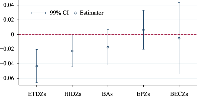
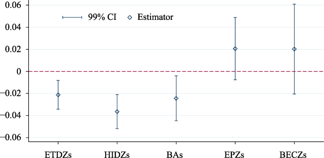
Figure 5 Heterogeneities among different types of national special economic zones

Notes: In the regressions of Figure 5, the dependent variable is Mono_a. We also run regressions using Mono_b as the dependent variable, and the results are highly similar to Figure 5, as shown in Figure C1 in Appendix C.

In China, SEZs are created with different pillar industries. This diversity in pillar industries within various types of SEZs gives rise to heterogeneous policy effects. We then distinguish between SEZs dominated by manufacturing and service industries and classify their pillar industries based on R&D intensity. Furthermore, we explore the heterogeneity of policy effects stemming from different pillar industries. The regression results are presented in Table 5.
Table 5 Heterogeneities among different pillar industries of special economic zones
(1) (2) (3)
Manufacturing SEZ -0.007***
(0.002)
Service SEZ -0.015*** -0.014***
(0.005) (0.005)
Medium-low manufacturing SEZ -0.001 -0.002
(0.003) (0.003)
Medium manufacturing SEZ -0.008** -0.009**
(0.004) (0.004)
Medium-high manufacturing SEZ -0.008*** -0.010***
(0.002) (0.002)
High manufacturing SEZ -0.007** -0.010***
(0.003) (0.003)
Controls Yes Yes Yes
County fixed effects Yes Yes Yes
Province-by-year fixed effects Yes Yes Yes
Number of counties 2164 2142 2164
R2 0.741 0.740 0.741
Observations 45,221 43,965 45,221

Notes: The standard errors are in parentheses and clustered at the county level. *, **, and *** denote significance levels of 10%, 5%, and 1%, respectively. The control variables are the same as those in Equation (3).

In Column (1), the SEZ effects are decomposed by examining the impacts of SEZs dominated by manufacturing and service industries. We find that both groups of SEZs have a significant negative impact on monocentricity. To understand the heterogeneities more clearly, we further classify manufacturing industry-oriented SEZs into four groups based on R&D intensity: medium-low, medium, medium-high, and high. The regression results are listed in Columns (2) and (3) of Table 5. We confirm that the negative impact of SEZs on monocentricity is driven by SEZs dominated by industries with medium and high R&D intensity, while SEZs dominated by industries with medium-low R&D intensity have no significant impact on urban spatial structure.
SEZs dominated by the service sector exhibit a stronger effect in reducing the monocentricity compared to their manufacturing counterparts. The pillar industries in these service-oriented SEZs encompass IT and other information services, software publishing, and other similar sectors. These industries effectively harness a diverse range of knowledge- based capital and draw upon a highly skilled workforce, which maintains strong direct and indirect multiplier effects. Therefore, the service-oriented SEZs yield the most potent policy impact on the urban structure.
For SEZs dominated by the manufacturing sector, SEZs hosting industries with higher R&D intensity can effectively promote a polycentric spatial structure. Given that the majority of SEZs are focused on manufacturing industries, the level of R&D intensity is closely linked to productivity in manufacturing activities. The goal of current development strategies in China is to incentivize enterprises to elevate their R&D intensity to drive economic growth. Enterprises with higher R&D intensity are more likely to leverage government tax incentives for resource acquisition. However, manufacturing-oriented SEZs with medium- low R&D intensity do not significantly impact spatial structure. These pillar industries with low R&D intensity are textiles, leather and related products, food products, beverages, tobacco, and others. These industries are labor intensive and have low multiplier effects.
Third, to understand the role of agglomeration economies, we investigate the heterogeneous effects of SEZs by age and size. Specifically, we interact SEZ dummies with age and size variables, and the results are listed in Table 6.
Table 6 Heterogeneities among special economic zones of different ages and sizes
(1) (2) (3) (4)
SEZ×age -0.002***
(0.000)
National SEZ×age -0.004***
(0.000)
Provincial SEZ×age -0.001***
(0.000)
SEZ×size -0.007***
(0.002)
National SEZ×size -0.027***
(0.005)
Provincial SEZ×size -0.003*
(0.002)
Controls Yes Yes Yes Yes
County fixed effects Yes Yes Yes Yes
Province-by-year fixed effects Yes Yes Yes Yes
Number of counties 2164 2164 2164 2164
R2 0.741 0.743 0.74 0.741
Observations 45,221 45,221 45,221 45,221

Notes: The standard errors are in parentheses and clustered at the county level. *, **, and *** denote significance levels of 10%, 5%, and 1%, respectively. The control variables are the same as those in Equation (3).

All regression coefficients in Table 6, including those for national and provincial SEZs, are significantly negative. This pattern indicates that the negative impact of SEZs on monocentric structure increases with the age and size of the SEZ. In other words, a longer duration of SEZ existence is associated with stronger policy effects of SEZs in reducing monocentricity. These findings align with the findings from the event study in Section 4.2. Columns (3) and (4) illustrate that larger SEZs contribute to a more pronounced and negative effects on monocentricity.
In summary, the results in Figure 5 and Tables 5 and 6 provide strong evidence for Hypothesis II. The SEZ effects on spatial structure vary with zone characteristics, including the type, pillar industries, age, and spatial size.

5.2 Heterogeneities by geographic location of zones

In China, the spatial patterns and intensity of economic activities are highly uneven within and among prefectures (Faber, 2014; Chang and Zheng, 2022). At a micro level, the intensity of economic activity and population density decrease as the distance from the CBD increases. At a macro-level, the density of urban areas is usually higher than that of peripheral counties, and top-tier cities generally have higher economic activity and population density than low-tier cities 7 . As a result, we expect that the impacts of the introduction of SEZs on urban spatial structure vary with geographic location.
To understand the spatial heterogeneities of SEZ effects at a micro-level, we first divide these zones into three groups based on their distance to the CBD and perform DID regressions with subsamples. The results are reported in Table 7. We only find statistically significant coefficients for national SEZs, which are consistent with the baseline findings in Table 3. Specifically, national SEZs significantly contribute to the decline in monocentric urban structure when located at a moderate distance from existing centers. Furthermore, in comparison to national SEZs located in close proximity to the CBD (within a distance of less than 5 km), national SEZs situated farther away from the CBD (more than 15 km) exhibit the ability to reduce a monocentric structure. This implies that the reduction in monocentricity is significant when the SEZ (new center) is relatively isolated from the preexisting center. However, the optimal scenario appears to be one where the new center maintains a moderate distance (5-15 km) from the existing center, as it can function as a new subcenter while also maintaining connectivity with the preexisting center. These findings are consistent with the literature (Zheng et al., 2019). Urban planners face cost and benefit trade-offs when locating new suburban centers. The spatial spillover effects of new subcenters decrease as the distance from the existing city center increases, but the corresponding construction costs also decrease, especially land costs (Zheng et al., 2019).
Table 7 Heterogeneities among different locations of special economic zones at a micro level
Distance to CBD
(1)
<5 km
(2)
5-15 km
(3)
>15 km
SEZ -0.003 -0.002 0.001
(0.003) (0.004) (0.006)
National SEZ -0.002 -0.033*** -0.017*
(0.008) (0.007) (0.010)
Provincial SEZ -0.004 -0.000 0.002
(0.003) (0.004) (0.007)
Controls Yes Yes Yes Yes Yes Yes
County fixed effects Yes Yes Yes Yes Yes Yes
Province-by-year fixed effects Yes Yes Yes Yes Yes Yes
Number of counties 1991 1991 1978 1978 1869 1869
R2 0.740 0.740 0.760 0.761 0.751 0.751
Observations 35,370 35,370 30,737 30,737 26,508 26,508

Notes: The standard errors are in parentheses and clustered at the county level. *, **, and *** denote significance levels of 10%, 5%, and 1%, respectively. The control variables are the same as those in Equation (3).

Second, to explore the heterogeneous effect of SEZs on the spatial structure between urban areas and peripheral counties, we allow the SEZ dummies to interact with urban and county indicators by applying Equation (3). The results are listed in Panel A of Table 8. Column (1) shows that monocentricity significantly decreases by approximately 1.3% in urban areas after the introduction of SEZs. The coefficient of SEZs in counties is slightly positive, with a 10% significance level. Column (2) confirms the findings that the significant impacts of SEZs on monocentricity are mainly observed in urban areas.
Third, we investigate the heterogeneity of SEZ effects among prefectures and include the interaction between the city tier indicators and SEZ dummies into Equation (3). The results are presented in Panel B of Table 8, which is organized similarly to Panel A. The results show that national SEZs have a significant impact on spatial structure in both top- and low-tier cities. However, the effects of provincial SEZs are insignificant in both top-tier and low-tier cities. These results are consistent with the baseline findings in Table 3.
Table 8 Spatial heterogeneities at a macro-level
Panel A: Urban areas vs.
Peripheral counties
Panel B: Top-tier cities vs. Low-tier cities
(1) (2) (3) (4)
SEZ×urban -0.013*** SEZ×top-tier 0.002
(0.005) (0.005)
SEZ×county 0.005* SEZ×low-tier 0.003
(0.003) (0.003)
National SEZ×urban -0.029*** National SEZ×top-tier -0.036**
(0.005) (0.011)
National SEZ×county -0.011 National SEZ×low-tier -0.020*
(0.008) (0.005)
Provincial SEZ×urban -0.010** Provincial SEZ×top-tier -0.009
(0.005) (0.006)
Provincial SEZ×county 0.002 Provincial SEZ×low-tier 0.003
(0.003) (0.003)
Controls Yes Yes Controls Yes Yes
County fixed effects Yes Yes County fixed effects Yes Yes
Province-by-year fixed effects Yes Yes Province-by-year fixed effects Yes Yes
Number of counties 2164 2164 Number of counties 2164 2164
R2 0.74 0.741 R2 0.74 0.741
Observations 45,221 45,221 Observations 45,221 45,221

Notes: The standard errors are in parentheses and clustered at the county level. *, **, and *** denote significance levels of 10%, 5%, and 1%, respectively. The control variables are the same as those in Equation (3).

In general, the regression results in Tables 7 and 8 indicate that geographical location significantly affects SEZ effects on spatial structure. This proves that Hypothesis III is hold, especially for national zones.

6 Conclusions and discussion

6.1 Conclusions

The rapid growth of China is characterized by a mixture of elements of market and active government involvement in stimulating investment and technology integration. The role of development policies and government intervention holds crucial significance in China, and the empirical evidence provided by this study confirms that place-based policies potentially play an important role in shaping urban spatial structure during urban growth.
As a crucial place-based policy pursued by the Chinese government as a development strategy, SEZ policy has made significant contributions to regional growth. Utilizing long- term nighttime light images to measure urban spatial structure and regarding the establishment of SEZs as the treatment policy, this study quantifies the causal effects of SEZs on urban spatial structure. Using county-level data from 2000-2020 in a set of time-varying DID estimations, we find that the introduction of national SEZs has a significant negative impact on monocentricity. In other words, the establishment of SEZs in China can serve as an effective tool in fostering polycentric development. However, the average effect of SEZs masks substantial heterogeneity with respect to the characteristics and geographic location of zones. Table 9 summarizes the heterogeneities and reports the significance levels of SEZ effects on spatial structure.
Table 9 Summary of empirical findings: Impacts of special economic zones on polycentricity
SEZs National SEZs Provincial SEZs
Panel A: Average effect
Overall ✔✔✔
Panel B: Heterogeneities by zone types and pillar industries of zones
ETDZs ✔✔✔
HIDZs ✔✔✔
BAs
EPZs
BECZs
Panel C: Heterogeneities by pillar industries of zones
Manufacturing ✔✔✔
Medium-low
Medium ✔✔
Medium-high ✔✔✔
High ✔✔✔
Service IDZ ✔✔✔
Panel D: Heterogeneities by age and size of zones
Age ✔✔✔ ✔✔✔ ✔✔✔
Size ✔✔✔ ✔✔✔
Panel E: Heterogeneities by geographic locations of zones (Micro-level)
Distance to CBD<5 km
5 km<Distance to CBD<15 km ✔✔✔
Distance to CBD>15 km
Panel F: Heterogeneities by geographic locations of zones (Macro-level)
Urban areas ✔✔✔ ✔✔✔ ✔✔
Peripheral counties
Top-tier cities ✔✔
Low-tier cities

Notes: “✔” and “✘” represent positive and negative effects of the SEZ policy on polycentricity, respectively. In addition, “✔”, “✔✔”, and “✔✔✔” denote positive impacts with statistical significance levels of 10%, 5%, and 1%, respectively. Similarly, “✘”, “✘✘”, and “✘✘✘” denote negative impacts with statistical significance levels of 10%, 5%, and 1%, respectively. Table 9 summarizes the estimation results with Mono_a as the dependent variable. The regression results of Mono_b as the dependent variable are highly consistent with Table 9, and these results are available upon request.

Considering that SEZs are established to stimulate local growth and attract FDI, their influence on spatial structure becomes more pronounced when they have the ability to attract a greater number of firms and employees to form employment centers. In other words, the prerequisite for the introduction of SEZs as an effective policy tool to reduce monocentricity is good employment performance in SEZs. From the perspective of the administrative level, national SEZs, particularly ETZs and HIDZs, play a predominant role in reducing monocentricity. This is because they often receive more attractive preferential policies than other SEZs. However, the average effect of provincial SEZs is small and insignificant, and it takes longer (approximately 7 years) to generate a substantial impact on local spatial structure for provincial zones. The results of heterogeneity analysis confirm that these provincial SEZs, which are characterized by medium-high R&D intensity, large size, and old age, have better performance in reducing monocentricity. All of the abovementioned factors collectively amplify the policy effects on the urban spatial structure of all types of SEZs, as they tend to have high multiplier effects. Furthermore, when national SEZs are strategically positioned at a moderate distance (5-15 km) from the existing CBD, they exert a maximized influence on the reduction of monocentricity. This location allows an SEZ to maintain its independence while simultaneously fostering a strong connection with the existing CBD.

6.2 Discussion

This paper also provides empirical evidence on the time-lag effects of place-based policies. The results of both the event study and heterogeneity analysis reveal that the impact of the introduction of SEZs on urban spatial structure becomes significant after several years. On average, national SEZs show a significant impact on urban spatial structure 3 years after they commence operation, while provincial SEZs take 7 years to show significant performance after they are established. In China, half of the national zones are upgraded from well-performing provincial zones, and the average age of national SEZs was 6.7 years higher than the provincial zones. These facts explain the significant effects of national zones and insignificant effects of provincial zones well.
It is important to note that not all SEZs have significant performance, although their construction and operation consume substantial land and funds. Some scholars have noted that some place-based policies have produced less-than-desirable outcomes in the practices in developed countries (Busso et al., 2013), even though China’s case illustrates the success of such place-based policies and their crucial roles in urban growth (Zheng et al., 2017), which is closely tied to the unique institutional and market environment of China. Notably, there are also a large number of SEZs with low performance in China. The empirical evidence in this paper confirms that national SEZs significantly affect urban spatial structure, while provincial SEZs do not. This finding is consistent with the literature, which documents that the performance of provincial SEZs is significantly lower than that of national SEZs (Chen et al., 2022). These findings highlight that the introduction of SEZs alone is not sufficient as a growth catalyst in suburban and peripheral counties of developing countries. Instead, the high performance of SEZs depends on supporting planning efforts (such as coordination between pillar industries of SEZs and local industrial structure) and favorable local economic conditions (Frick et al., 2019). However, the mechanisms through which SEZs transition into sub-centers are not thoroughly discussed in this paper. More specific and comprehensive research is needed to verify these mechanisms and provide corresponding policy suggestions.
Finally, we highlight several analytical challenges for further studies. First, urban spatial structure can be measured by multiple dimensions, and mono-polycentricity is only one important dimension. Second, this paper focuses solely on the evaluation of the SEZ policy on urban spatial structure. While some SEZs may not significantly affect urban spatial structure, it is important to note that they may produce other significant performances, such as economic growth, population agglomeration, employment, productivity, and trade. Thus, a more comprehensive exploration of the effects of SEZ policy can be conducted in the future.

Appendix A

Figure A1 The results of event study using Mono_b as the dependent variable

Notes: 0 means the year when the first SEZ was launched, -1 represents the one year before SEZ operation and so on, and 1 refers to the time that is one year after SEZ operation.

Appendix B

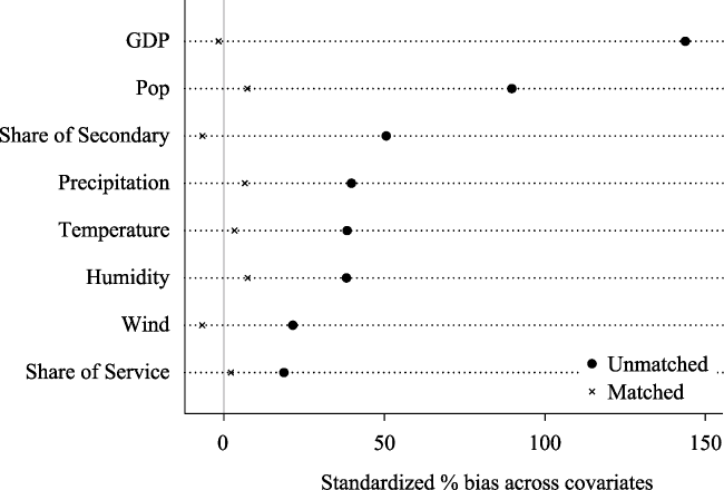
Figure B1 The results of propensity score matching
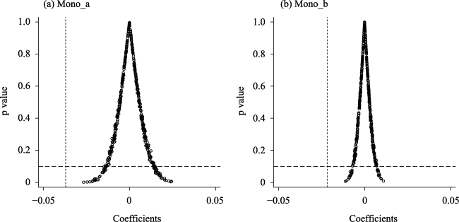
Figure B2 The results of placebo tests
Table B1 Results of Goodman-Bacon decomposition
Comparison type Weight Estimates Comparison type Weight Estimates
Earlier Treatment vs. Later Comparison 0.012 0.003 Treatment vs. Never treated 0.936 -0.059
Later Treatment vs. Earlier Comparison 0.009 0.002 Treatment vs. Already treated 0.043 0.000

Appendix C

Figure C1 Heterogeneities among different types of special economic zones using Mono_b as the dependent variable
[1]
Achten S, Lessmann C, 2020. Spatial inequality, geography and economic activity. World Development, 136: 105114.

[2]
Alder S, Shao L, Zilibotti F, 2016. Economic reforms and industrial policy in a panel of Chinese cities. Journal of Economic Growth, 21(4): 305-349.

[3]
Alonso W, 1964. Location and Land Use: Toward a General Theory of Land Rent. MA: Harvard University Press.

[4]
Anas A, Arnott R, Small K A, 1998. Urban spatial structure. Journal of Economic Literature, 36(3): 1426-1464.

[5]
Arribas-Bel D, Sanz-Gracia F, 2014. The validity of the monocentric city model in a polycentric age: US metropolitan areas in 1990, 2000 and 2010. Urban Geography, 35(7): 980-997.

[6]
Baker A C, Larcker D F, Wang C C Y, 2022. How much should we trust staggered difference-in-differences estimates? Journal of Financial Economics, 144(2): 370-395.

[7]
Baum-Snow N, Brandt L, Henderson J V et al., 2017. Roads, railroads, and decentralization of Chinese cities. Review of Economics and Statistics, 99(3): 435-448.

[8]
Busso M, Gregory J, Kline P, 2013. Assessing the incidence and efficiency of a prominent place based policy. American Economic Review, 103(2): 897-947.

[9]
Cao G, Shi Q, Liu T, 2016. An integrated model of urban spatial structure: Insights from the distribution of floor area ratio in a Chinese city. Applied Geography, 75: 116-126.

[10]
Ch R, Martin D A, Vargas J F, 2021. Measuring the size and growth of cities using nighttime light. Journal of Urban Economics, 125: 103254.

[11]
Chang Z, Deng C, Long F et al., 2021. High-speed rail, firm agglomeration, and PM2.5: Evidence from China. Transportation Research Part D: Transport and Environment, 96: 102886.

[12]
Chang Z, Zheng L, 2022. High-speed rail and the spatial pattern of new firm births: Evidence from China. Transportation Research Part A: Policy and Practice, 155: 373-386.

[13]
Chang Z, Zheng L, Yang T et al., 2022. High-speed rail, new town development, and the spatial mismatch of land leases in China. Land Use Policy, 115: 106014.

[14]
Chen T, Hui E C M, Wu J et al., 2019. Identifying urban spatial structure and urban vibrancy in highly dense cities using georeferenced social media data. Habitat International, 89: 102005.

[15]
Chen W, Su Z, Wang Y et al., 2022. Do the rank difference of industrial development zones affect land use efficiency? A regional analysis in China. Socio-Economic Planning Sciences, 80: 101168.

[16]
Chen Z, Yu B, Yang C et al., 2021. An extended time series (2000-2018) of global NPP-VIIRS-like nighttime light data from a cross-sensor calibration. Earth System Science Data, 13(3): 889-906.

[17]
Cheng H, Liu Y, He S et al., 2017. From development zones to edge urban areas in China: A case study of Nansha, Guangzhou city. Cities, 71: 110-122.

[18]
Cheng J, Masser I, 2003. Urban growth pattern modeling: A case study of Wuhan city, PR China. Landscape and Urban Planning, 62(4): 199-217.

[19]
Dadashpoor H, Azizi P, Moghadasi M, 2019. Analyzing spatial patterns, driving forces and predicting future growth scenarios for supporting sustainable urban growth: Evidence from Tabriz metropolitan area, Iran. Sustainable Cities and Society, 47: 101502.

[20]
Ding C, Zhao X, 2014. Land market, land development and urban spatial structure in Beijing. Land Use Policy, 40: 83-90.

[21]
Du J, Thill J C, Peiser R B et al., 2014. Urban land market and land-use changes in post-reform China: A case study of Beijing. Landscape and Urban Planning, 124: 118-128.

[22]
Duranton G, Venables A J, 2018. Place-based policies for development. NBER Working Paper 24562.

[23]
Faber B, 2014. Trade integration, market size, and industrialization: Evidence from China’s National Trunk Highway System. The Review of Economic Studies, 81(3): 1046-1070.

[24]
Fang X, Su D, Wu Q et al., 2023. Dynamic changes in urban land spatial inequality under the core-periphery structure in urban agglomerations. Journal of Geographical Sciences, 33(4): 760-778.

DOI

[25]
Fei W, Zhao S, 2019. Urban land expansion in China’s six megacities from 1978 to 2015. Science of The Total Environment, 664: 60-71.

[26]
Frick S A, Rodríguez-Pose A, Wong M D, 2019. Toward economically dynamic special economic zones in emerging countries. Economic Geography, 95(1): 30-64.

[27]
Fujita M, Thisse J F, Zenou Y, 1997. On the endogeneous formation of secondary employment centers in a city. Journal of Urban Economics, 41(3): 337-357.

[28]
Glaeser E L, Kahn M E, 2001. Decentralized employment and the transformation of the American city. NBER Working Paper w8117.

[29]
Goodman-Bacon A, 2021. Difference-in-differences with variation in treatment timing. Journal of Econometrics, 225(2): 254-277.

[30]
Gordon P, Richardson H W, Wong H L, 1986. The distribution of population and employment in a polycentric city: The case of Los Angeles. Environment and Planning A: Economy and Space, 18(2): 161-173.

[31]
Gu C, Hu L, Cook I G, 2017. China’s urbanization in 1949-2015: Processes and driving forces. Chinese Geographical Science, 27(6): 847-859.

[32]
Hajrasouliha A H, Hamidi S, 2017. The typology of the American metropolis: Monocentricity, polycentricity, or generalized dispersion? Urban Geography, 38(3): 420-444.

[33]
Han S, Sun B, Zhang T, 2020. Mono- and polycentric urban spatial structure and PM2.5 concentrations: Regarding the dependence on population density. Habitat International, 104: 102257.

[34]
Howell A, 2019. Heterogeneous impacts of China’s economic and development zone program. Journal of Regional Science, 59(5): 797-818.

[35]
Huang D, He H, Liu T, 2021a. City size and employment dynamics in China: Evidence from recruitment website data. Journal of Geographical Sciences, 31(12): 1737-1756.

[36]
Huang D, Liu T, Kong F et al., 2021b. Employment centers change faster than expected: An integrated identification method and application to Beijing. Cities, 115: 103224.

[37]
Huang D, Liu Z, Zhao X et al., 2017. Emerging polycentric megacity in China: An examination of employment subcenters and their influence on population distribution in Beijing. Cities, 69: 36-45.

[38]
Kline P, Moretti E, 2014. People, places, and public policy: Some simple welfare economics of local economic development programs. Annual Review of Economics, 6(1): 629-662.

[39]
Lee B, 2007. “Edge” or “edgeless” cities? Urban spatial structure in US metropolitan areas, 1980 to 2000. Journal of Regional Science, 47(3): 479-515.

[40]
Lee N, Rodríguez-Pose A, 2013. Innovation and spatial inequality in Europe and USA. Journal of Economic Geography, 13(1): 1-22.

[41]
Li W, Sun B, Zhang T, 2018a. Spatial structure and labour productivity: Evidence from prefectures in China. Urban Studies, 56(8): 1516-1532.

[42]
Li W, Sun B, Zhang T et al., 2022. Polycentric spatial structure and its economic performance: Evidence from meta-analysis. Regional Studies, 56(11): 1888-1902.

[43]
Li W, Sun B, Zhao J et al., 2018b. Economic performance of spatial structure in Chinese prefecture regions: Evidence from night-time satellite imagery. Habitat International, 76: 29-39.

[44]
Li Y, 2020. Towards concentration and decentralization: The evolution of urban spatial structure of Chinese cities, 2001-2016. Computers, Environment and Urban Systems, 80: 101425.

[45]
Li Y, Derudder B, 2022. Dynamics in the polycentric development of Chinese cities, 2001-2016. Urban Geography, 43(2): 272-292.

[46]
Li Y, Du R, 2022. Polycentric urban structure and innovation: Evidence from a panel of Chinese cities. Regional Studies, 56(1): 113-127.

[47]
Li Y, Liu X, 2018. How did urban polycentricity and dispersion affect economic productivity? A case study of 306 Chinese cities. Landscape and Urban Planning, 173: 51-59.

[48]
Li Y, Zhu K, Wang S, 2020. Polycentric and dispersed population distribution increases PM2.5 concentrations: Evidence from 286 Chinese cities, 2001-2016. Journal of Cleaner Production, 248: 119202.

[49]
Liu X, Wang M, 2016. How polycentric is urban China and why? A case study of 318 cities. Landscape and Urban Planning, 151: 10-20.

[50]
Liu Z, Liu S, 2018. Polycentric development and the role of urban polycentric planning in China’s mega cities: An examination of Beijing’s metropolitan area. Sustainability, 10(5): 1588.

[51]
Long F, Zheng L, Song Z, 2018. High-speed rail and urban expansion: An empirical study using a time series of nighttime light satellite data in China. Journal of Transport Geography, 72: 106-118.

[52]
Long Y, 2016. Redefining Chinese city system with emerging new data. Applied Geography, 75: 36-48.

[53]
Lu F, Sun W, Wu J, 2023. Special economic zones and human capital investment: 30 years of evidence from China. American Economic Journal: Economic Policy, 15(3): 35-64.

[54]
Lu Y, Wang J, Zhu L, 2019. Place-based policies, creation, and agglomeration economies: Evidence from China’s economic zone program. American Economic Journal: Economic Policy, 11(3): 325-360.

[55]
Ma S, Long Y, 2020. Functional urban area delineations of cities on the Chinese mainland using massive Didi ride-hailing records. Cities, 97: 102532.

[56]
Meijers E, 2008. Measuring polycentricity and its promises. European Planning Studies, 16(9): 1313-1323.

[57]
Meijers E J, Burger M J, 2010. Spatial structure and productivity in US metropolitan areas. Environment and Planning A: Economy and Space, 42(6): 1383-1402.

[58]
Münter A, Volgmann K, 2020. Polycentric regions: Proposals for a new typology and terminology. Urban Studies, 58(4): 677-695.

[59]
Nijman J, Wei Y D, 2020. Urban inequalities in the 21st century economy. Applied Geography, 117: 102188.

[60]
Qin Y, 2017. ‘No county left behind?’ The distributional impact of high-speed rail upgrades in China. Journal of Economic Geography, 17(3): 489-520.

[61]
Salvati L, Zambon I, Chelli F M et al., 2018. Do spatial patterns of urbanization and land consumption reflect different socioeconomic contexts in Europe? Science of The Total Environment, 625: 722-730.

[62]
Schminke A, Biesebroeck J V, 2013. Using export market performance to evaluate regional preferential policies in China. Review of World Economics, 149(2): 343-367.

[63]
Small K A, Song S, 1994. Population and employment densities: Structure and change. Journal of Urban Economics, 36(3): 292-313.

[64]
Sun Y, Ma A, Su H et al., 2020. Does the establishment of development zones really improve industrial land use efficiency? Implications for China’s high-quality development policy. Land Use Policy, 90: 104265.

[65]
Wang J, 2013. The economic impact of special economic zones: Evidence from Chinese municipalities. Journal of Development Economics, 101(1): 133-147.

[66]
Wang S, Luo X, 2022. The evolution of government behaviors and urban expansion in Shanghai. Land Use Policy, 114: 105973.

[67]
Wang Z, Kong X, Cheng P, 2022. Spatiotemporal evolution of national development zones and their impact on urban land growth in China. Journal of Geographical Sciences, 32(8): 1451-1470

DOI

[68]
Wu C, Smith D, Wang M, 2021. Simulating the urban spatial structure with spatial interaction: A case study of urban polycentricity under different scenarios. Computers, Environment and Urban Systems, 89: 101677.

[69]
Wu F, Yeh A G O, 1999. Urban spatial structure in a transitional economy: The case of Guangzhou, China. Journal of the American Planning Association, 65(4): 377-394.

[70]
Zeng D Z, 2021. The past, present, and future of special economic zones and their impact. Journal of International Economic Law, 24(2): 259-275.

[71]
Zhang T, Sun B, Li W, 2017. The economic performance of urban structure: From the perspective of polycentricity and monocentricity. Cities, 68: 18-24.

[72]
Zhao P, Diao J, Li S, 2017. The influence of urban structure on individual transport energy consumption in China’s growing cities. Habitat International, 66: 95-105.

[73]
Zheng G, Barbieri E, Tommaso M R D et al., 2016. Development zones and local economic growth: Zooming in on the Chinese case. China Economic Review, 38: 238-249.

[74]
Zheng L, Chang Z, Martinez A G, 2022. High-speed rail, market access, and the rise of consumer cities: Evidence from China. Transportation Research Part A: Policy and Practice, 165: 454-470.

[75]
Zheng L, Long F, Chang Z et al., 2019. Ghost town or city of hope? The spatial spillover effects of high-speed railway stations in China. Transport Policy, 81: 230-241.

[76]
Zheng L, Pan F, 2024. Does place-based policy increase new firm births? Evidence from special economic zones in China. Applied Geography, 168: 103303.

[77]
Zheng L, Wu S, 2024. Remote high-speed rail stations, urban land supply, and the emergence of new economic activities. Transportation Research Part A: Policy and Practice, 189: 104226.

[78]
Zheng S, Sun W, Wu J et al., 2017. The birth of edge cities in China: Measuring the effects of industrial parks policy. Journal of Urban Economics, 100: 80-103.

[79]
Zhou H, Sun B, Zhang T, 2024. The evolution of urban employment spatial structure in China: From the perspective of monocentricity and polycentricity. Cities, 147: 104824.

Outlines

/