
Journal of Geographical Sciences >
Differential evolution of territorial space and effects on ecological environment quality in China’s border regions
|
Gu Guanhai, Master, specialized in land use and regional development. E-mail: gguanhai@163.com |
Received date: 2023-06-09
Accepted date: 2023-12-27
Online published: 2024-09-11
Supported by
National Natural Science Foundation of China(42261043)
National Natural Science Foundation of China(42361047)
The Central Government Guides Local Funds For Science and Technology Development(ZY23055016)
Nanning Normal University High-Level Talent Team Project on Territorial Space Use and Geopolitical Security
Guangxi Zhuang Autonomous Region Doctoral and Master’s Graduate Education Innovation Plan Funding Project(YCSW2023433)
The use of territories in border areas is sensitive, unique, and ecologically fragile. A scientific understanding of the transformation of the national territorial space and its ecological and environmental responses is crucial for optimizing spatial patterns and promoting sustainable utilization. This study focused on 45 cities in the land border areas of China and employed techniques such as the land transfer matrix, Theil index, and ecological environment index to explore the spatiotemporal evolution process and eco-environmental effects of territorial space from three dimensions: spatial pattern, structural transformation, and ecological response. The results show that: (1) During the study period, there was an increasing trend in living and production space, along with a decrease in ecological space, and a significant pattern of "one belt, three districts, and multipoints" emerged. (2) In the urbanization process, population growth and industrial agglomeration have led to the transformation and conflict of territorial spaces, with the conversion of ecological spaces into production spaces being the primary form of land-use transformation. Rapid development has resulted in spatial differentiation of the territorial space between regions. (3) During this period, the ecological quality in China’s border areas deteriorated, yet the distribution pattern of ecological space remained stable, exhibiting a “high value in the southeast, low value in the northwest” pattern. (4) Improvements and degradation of the ecology coexist in different border areas; transforming agricultural production space into green and potential ecological spaces has positively contributed to enhancing ecological quality. In contrast, converting green ecological space into potential ecological space, agricultural production space, and aquatic ecological space has become a key factor in ecological degradation. Therefore, the border areas of China should utilize national preferential policies and strategies, recognize the vast and varied expanse of China’s border areas, and adopt differentiated planning and management measures in different regions to achieve the coordinated development of the PLES, thus promoting a positive trend in eco-environmental quality.
GU Guanhai , WU Bin , LU Shengquan , ZHANG Wenzhu , TIAN Yichao , LU Rucheng , FENG Xiaoling , LIAO Wenhui . Differential evolution of territorial space and effects on ecological environment quality in China’s border regions[J]. Journal of Geographical Sciences, 2024 , 34(6) : 1109 -1127 . DOI: 10.1007/s11442-024-2241-z
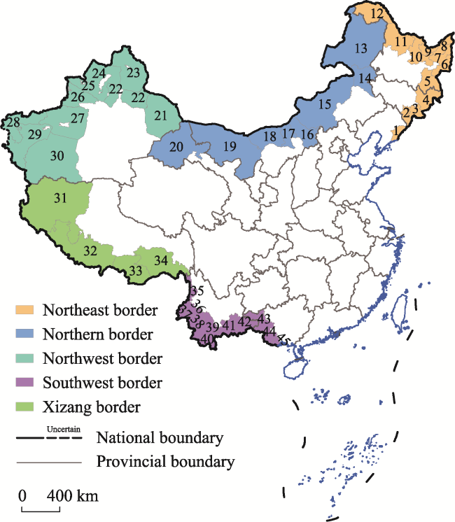
Figure 1 Schematic diagram of the study area (China’s border areas)Note: Numbers 1 to 45 represent the following respectively: 1. Dandong City, 2. Tonghua City, 3. Baishan City, 4. Yanbian Korean Autonomous Prefecture, 5. Mudanjiang City, 6. Jixi City, 7. Jiamusi City, 8. Shuangyashan City, 9. Hegang City, 10. Yichun City, 11. Heihe City, 12. Daxing’anling Prefecture, 13. Hulunbuir City, 14. Xing’an League, 15. Xilinkuole League, 16. Ulanqab City, 17. Baotou City, 18. Bayannur City, 19. Alxa League, 20. Jiuquan City, 21. Hami City, 22. Changji Hui Autonomous Prefecture, 23. Altay Prefecture, 24. Tacheng Prefecture, 25. Bortala Mongol Autonomous Prefecture, 26. Ili Kazakh Autonomous Prefecture, 27. Aksu Prefecture, 28. Kizilsu Kirghiz Autonomous Prefecture, 29. Kashgar Prefecture, 30. Hotan Prefecture, 31. Ngari Prefecture, 32. Shigatse City, 33. Shannan City, 34. Nyingchi City, 35. Nujiang Lisu Autonomous Prefecture, 36. Baoshan City, 37. Dehong Dai and Jingpo Autonomous Prefecture, 38. Lincang City, 39. Pu’er City, 40. Xishuangbanna Dai Autonomous Prefecture, 41. Honghe Hani and Yi Autonomous Prefecture, 42. Wenshan Zhuang and Miao Autonomous Prefecture, 43. Baise City, 44. Chongzuo City, 45. Fangchenggang City. The map is derived from the standard map with approval number GS(2019)1822 obtained from the Ministry of Natural Resources website, with an unaltered base map. |
Table 1 Data sources and description in this study |
| Data name | Data description | Data source |
|---|---|---|
| Land use/cover data | Raster data | Data Center for Resources and Environmental Sciences, Chinese Academy of Sciences (RESDC) (http://www.resdc.cn/) |
| NDVI | Raster data | |
| GPP | Raster data | |
| Socioeconomic data | Statistical data of prefecture-level cities in border areas | National Bureau of Statistics (NBS) (http://www.stats.gov.cn/) |
| DEM data | Raster data | Geospatial Data Cloud (http://www.gscloud.cn/) |
| Administrative boundary | Vector | Geographical lnformation Monitoring Cloud Platform (http://www.dsac.cn/) |
Table 2 Classification system of the territorial space in China’s border areas |
| First classification | Secondary classification | Land use type |
|---|---|---|
| Production space (PS) | Agricultural production space(APS) | Paddy field, dry land |
| Industrial and mining production space (IPS) | Industrial and mining land and its subsidiary transportation land | |
| Living space (LS) | Urban living space (ULS) | Urban land |
| Rural living space (RLS) | Rural residents land | |
| Ecological space (ES) | Greenland ecological space (GES) | Forestland, shrubs, sparse forestland, other forestland, high-coverage grassland, medium-coverage grassland, low-coverage grassland |
| Waters ecological space (WES) | Channel, lakes, pit ponds, beaches, beaches, beaches | |
| Potential ecological space (PES) | Naked land, nude rock texture, sand land, saline-alkali land, other unused land |
Table 3 Inicator system for measuring the ecological environment index |
| Indicators | Indicator Interpretation | Data processing |
|---|---|---|
| Ecological Quality Index (EQI) | The quantitative relationship between land use/land cover and ecological environment quality is constructed to characterize the overall ecological environment quality in the region | $EQ{{I}_{t}}=\left( \sum\limits_{i=1}^{n}{LU{{A}_{i,t}}\times E{{V}_{i,t}}} \right)/\sum\limits_{i=1}^{n}{LU{{A}_{i,t}}}$ (8) where EVt represents the corresponding ecological environmental quality assignment at time t for category i land use type; LUAt represents the area at time t for category i land use type. |
| Normalized Difference Vegetation Index (NDVI) | Indicators reflecting the degree of surface vegetation cover and the state of vegetation growth calculated by remote sensing data. | $NDVI=\left( NIR-R \right)/\left( NIR+R \right)$ (9) where NIR denotes the reflectance in the near-infrared band, and R denotes the reflectance in the red light band. |
| Total primary productivity of the ecosystem (GPP) | It is used to study the differences in productivity of different regions and ecosystems and to assess the functioning and stability of ecosystems. | $GPP=PAR\times FPAR\times \varepsilon $ (10) where PAR is photosynthetically active radiation, FPAR is the ratio of photosynthetically active radiation absorbed by vegetation, and ε is the realistic light energy utilization rate based on the GPP concept. |
Table 4 The proportion of territorial space area in China’s border areas from 1980 to 2020 (%) |
| PLES | 1980 | 1990 | 2000 | 2010 | 2020 | |
|---|---|---|---|---|---|---|
| PS | IPS | 0.02 | 0.02 | 0.02 | 0.07 | 0.15 |
| APS | 6.47 | 6.91 | 7.5 | 8.18 | 8.49 | |
| LS | ULS | 0.05 | 0.06 | 0.07 | 0.12 | 0.14 |
| RLS | 0.33 | 0.36 | 0.36 | 0.36 | 0.4 | |
| ES | GES | 57.6 | 57.26 | 56.58 | 51.32 | 52.34 |
| PES | 33.06 | 32.93 | 32.96 | 37.57 | 36.09 | |
| WPS | 2.46 | 2.46 | 2.5 | 2.39 | 2.41 | |
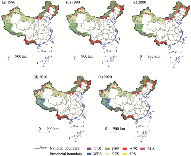
Figure 2 Territorial spatial pattern of China’s border areas from 1980 to 2020 |
Table 5 China’s Land Border Area Territory spatial pattern from the Patrol Theil Index for 1980-2020 |
| Terr Index | Territorial space | 1980 | 1990 | 2000 | 2010 | 2020 |
|---|---|---|---|---|---|---|
| Group Thiel Index | PS | 0.3567 | 0.3675 | 0.3774 | 0.3371 | 0.3324 |
| LS | 0.3690 | 0.3654 | 0.3351 | 0.2670 | 0.2344 | |
| ES | 0.1984 | 0.2030 | 0.2080 | 0.2101 | 0.2091 | |
| Tama Thiel Index | PS | 0.1121 | 0.1243 | 0.1413 | 0.1221 | 0.1130 |
| LS | 0.3581 | 0.3548 | 0.3376 | 0.2851 | 0.2659 | |
| ES | 0.3313 | 0.3378 | 0.3443 | 0.3437 | 0.3497 | |
| Northeast Border Thiel Index | PS | 0.3149 | 0.3429 | 0.3640 | 0.3806 | 0.3498 |
| LS | 0.1284 | 0.1100 | 0.1040 | 0.0774 | 0.0775 | |
| ES | 0.2108 | 0.2276 | 0.2429 | 0.2436 | 0.2483 | |
| Northern Border Theil index | PS | 0.3718 | 0.3923 | 0.4199 | 0.3359 | 0.3271 |
| LS | 0.3834 | 0.3844 | 0.3809 | 0.3425 | 0.2960 | |
| ES | 0.3372 | 0.3379 | 0.3412 | 0.3438 | 0.3409 | |
| Northwest Border Thiel Index | PS | 0.2871 | 0.2857 | 0.2869 | 0.2578 | 0.2531 |
| LS | 0.4161 | 0.4180 | 0.3434 | 0.2979 | 0.2788 | |
| ES | 0.1706 | 0.1707 | 0.1714 | 0.1773 | 0.1788 | |
| Xizang Border Thiel Index | PS | 0.9965 | 0.9966 | 0.9962 | 0.7109 | 0.6263 |
| LS | 0.2492 | 0.2491 | 0.2726 | 0.2050 | 0.1460 | |
| ES | 0.1256 | 0.1256 | 0.1256 | 0.1274 | 0.1274 | |
| Southwest Border Thiel Index | PS | 0.2217 | 0.2217 | 0.2182 | 0.2268 | 0.2824 |
| LS | 0.6108 | 0.6143 | 0.5635 | 0.4136 | 0.3527 | |
| ES | 0.1356 | 0.1359 | 0.1363 | 0.1364 | 0.1278 |
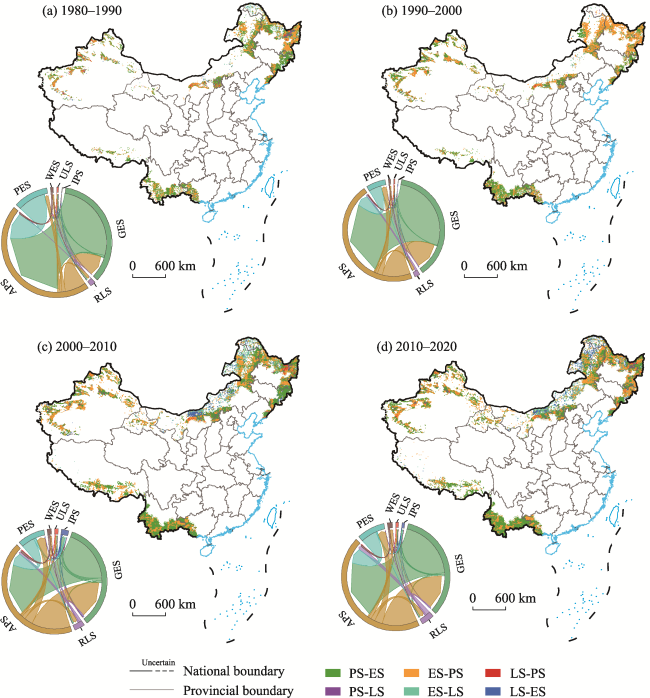
Figure 3 Territorial spatial structure conversion along China’s border areas from 1980 to 2020Note: PS, LS, ESL, APS, IPS, ULS, RLS, GES, WES and PES refer to the territorial classification rules in Table 2. |
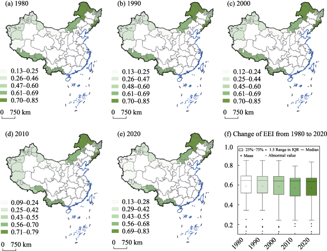
Figure 4 Spatio-temporal changes of the eco-environmental quality index in China’s border areasNote: a-e represent the spatial distribution changes of the eco-environmental quality index from 1980 to 2020, while f depicts the boxplot changes of the eco-environmental quality index. |
Table 6 Main territorial spatial transformations affecting the quality of the eco-environment and contribution rates |
| Lead to the improvement of the ecological environment | Lead to the deterioration of the ecological environment | ||||
|---|---|---|---|---|---|
| Structural transformation | Index movement | Proportion (%) | Structural transformation | Index movement | Proportion (%) |
| RPS-GES | 0.005921624 | 5.5524 | GES-PES | -0.042690174 | 72.7881 |
| PES-GES | 0.000754629 | 2.3360 | GPS-APS | -0.042690174 | 10.8501 |
| APS-PES | 0.005921624 | 1.4004 | GES-WES | -0.042690174 | 6.1888 |
| PES-WPS | 0.000754629 | 0.2097 | GES-RLS | -0.042690174 | 0.2560 |
| RPS-RLS | 0.005921624 | 0.1516 | WES-GES | -0.000275107 | 0.0622 |
| APS-WPS | 0.005921624 | 0.0851 | WPS-PES | -0.000275107 | 0.0464 |
| PES-APS | 0.000754629 | 0.0168 | GES-IPS | -0.042690174 | 0.0231 |
| APS-ULS | 0.005921624 | 0.0063 | GES-ULS | -0.042690174 | 0.0156 |
| APS-IPS | 0.005921624 | 0.0033 | WES-APS | -0.000275107 | 0.0052 |
| Summation | 9.7615 | Summation | 90.2355 | ||
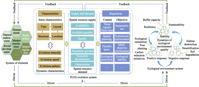
Figure 5 The mechanism of action between PLES and the ecological environment |
| [1] |
|
| [2] |
|
| [3] |
|
| [4] |
|
| [5] |
|
| [6] |
|
| [7] |
|
| [8] |
|
| [9] |
|
| [10] |
|
| [11] |
|
| [12] |
|
| [13] |
|
| [14] |
|
| [15] |
|
| [16] |
|
| [17] |
|
| [18] |
|
| [19] |
|
| [20] |
|
| [21] |
|
| [22] |
|
| [23] |
|
| [24] |
|
| [25] |
|
| [26] |
|
| [27] |
|
| [28] |
|
| [29] |
|
| [30] |
|
| [31] |
|
| [32] |
|
| [33] |
|
| [34] |
|
| [35] |
|
| [36] |
|
| [37] |
|
| [38] |
|
| [39] |
|
| [40] |
|
/
| 〈 |
|
〉 |