
Journal of Geographical Sciences >
Transfer learning framework for streamflow prediction in large-scale transboundary catchments: Sensitivity analysis and applicability in data-scarce basins
|
Ma Kai (1992-), PhD, specialized in transboundary hydrology and hydrologic modelling. E-mail: makai@ynu.edu.cn |
Received date: 2023-09-21
Accepted date: 2024-01-12
Online published: 2024-05-31
Supported by
National Key Research and Development Program of China(2022YFF1302405)
National Natural Science Foundation of China(42201040)
The National Key Research and Development Program of China(2016YFA0601601)
The China Postdoctoral Science Foundation(2023M733006)
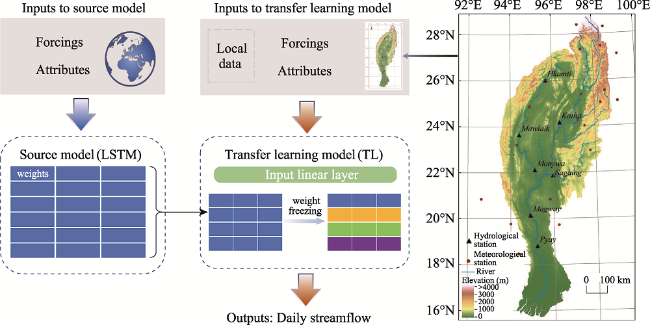
The imbalance in global streamflow gauge distribution and regional data scarcity, especially in large transboundary basins, challenge regional water resource management. Effectively utilizing these limited data to construct reliable models is of crucial practical importance. This study employs a transfer learning (TL) framework to simulate daily streamflow in the Dulong-Irrawaddy River Basin (DIRB), a less-studied transboundary basin shared by Myanmar, China, and India. Our results show that TL significantly improves streamflow predictions: the optimal TL model achieves an average Nash-Sutcliffe efficiency of 0.872, showing a marked improvement in the Hkamti sub-basin. Despite data scarcity, TL achieves a mean NSE of 0.817, surpassing the 0.655 of the process-based model MIKE SHE. Additionally, our study reveals the importance of source model selection in TL, as different parts of the flow are affected by the diversity and similarity of data in the source model. Deep learning models, particularly TL, exhibit complex sensitivities to meteorological inputs, more accurately capturing non-linear relationships among multiple variables than the process-based model. Integrated gradients (IG) analysis further illustrates TL’s ability to capture spatial heterogeneity in upstream and downstream sub-basins and its adeptness in characterizing different flow regimes. This study underscores the potential of TL in enhancing the understanding of hydrological processes in large-scale catchments and highlights its value for water resource management in transboundary basins under data scarcity.
MA Kai , SHEN Chaopeng , XU Ziyue , HE Daming . Transfer learning framework for streamflow prediction in large-scale transboundary catchments: Sensitivity analysis and applicability in data-scarce basins[J]. Journal of Geographical Sciences, 2024 , 34(5) : 963 -984 . DOI: 10.1007/s11442-024-2235-x
Figure 1 Transfer learning framework based on LSTM model and the location and observation stations of Dulong-Irrawaddy River Basin |
Table 1 The Nash-Sutcliffe Efficiency (NSE) of all sub-basins for LSTM and optimal TLs with different source models |
| Models | Hkamti | Mawlaik | Monywa | Katha | Sagaing | Magway | Pyay |
|---|---|---|---|---|---|---|---|
| LSTM | 0.755 | 0.848 | 0.817 | 0.826 | 0.840 | 0.878 | 0.865 |
| TL (US) | 0.844 | 0.863 | 0.865 | 0.876 | 0.855 | 0.902 | 0.896 |
| TL (GB) | 0.778 | 0.875 | 0.885 | 0.854 | 0.841 | 0.916 | 0.909 |
| TL (CL) | 0.857 | 0.858 | 0.860 | 0.876 | 0.855 | 0.903 | 0.894 |
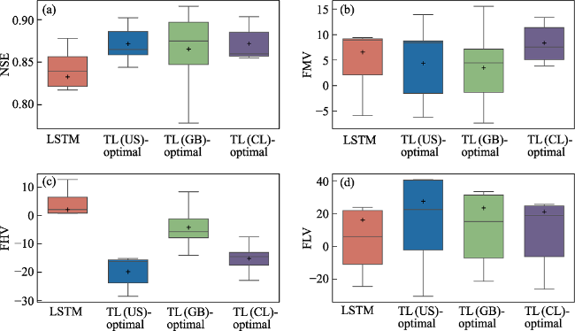
Figure 2 Performance comparison between LSTM and TLs with different source models. Panel (a) displays the Nash-Sutcliffe Efficiency (NSE) of both LSTM and TL models for the ensemble mean discharge of five members during the test period. Panel (b) illustrates the percentage bias within the 20%-80% flow range (FMV). Panel (c) reveals the percentage bias within the top 2% peak flow range (FHV), while panel (d) represents the percentage bias within the bottom 2% low flow range (FLV). The median value is indicated by the central line, while a plus sign (+) typically represents the mean NSE. |
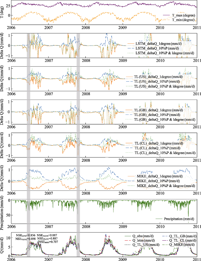
Figure 3 Sensitivity of LSTM, TL and MIKE SHE models in Pyay. It shows the streamflow simulations of different models at the outlet of the DIRB (Pyay) (panel 8) and their observed changes in temperature (panel 1) and rainfall (panel 7). Panels 2-6 show the streamflow changes (Delta) of the machine learning model (LSTM and TL using different source data) and MIKE SHE in the set scenarios, respectively. The shaded sections in the figure highlight examples where extremes in temperature sensitivity align with peak occurrences of rainfall and flow events. |
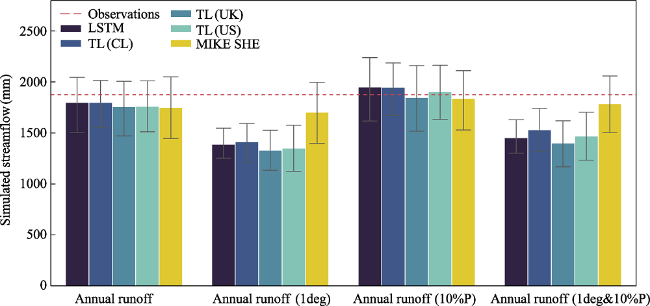
Figure 4 The multi-year annual runoff of Pyay simulated by LSTM, TLs, and MIKE SHE during the test period. The red dashed line represents the observed streamflow during the test years (mm). |
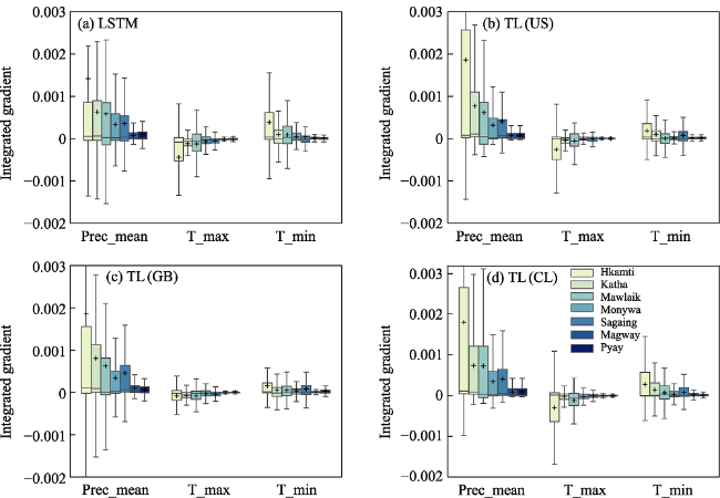
Figure 5 The integrated gradient (IG) of different forcing variables for LSTM (a), TL(US) (b), TL(GB) (c), and TL(CL) (d) in each sub-basin is illustrated, with the color deepening as the latitude of the sub-basin decreases. |
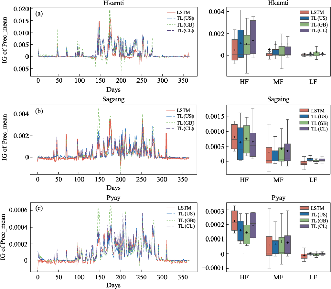
Figure 6 The integrated gradient of precipitation for LSTM and TLs in (a) Hkamti, (b) Sagaing, and (c) Pyay. The box diagrams highlight the IG values corresponding to the top 2% high-flow (HF), 20%-80% mid-flow (MF), and bottom 30% low-flow (LF) part. |
Table 2 The performance of MIKE SHE, LSTM and optimal TLs trained with different source models for data deficit scenario |
| Models | NSE | FHV | FLV | FMV |
|---|---|---|---|---|
| MIKE SHE | 0.655 | -20.952 | 38.498 | 5.893 |
| LSTM | 0.774 | -22.909 | 47.278 | 10.662 |
| TL(US) | 0.816 | -24.907 | 50.782 | 0.757 |
| TL(GB) | 0.816 | -20.539 | 45.416 | 7.205 |
| TL(CL) | 0.817 | -23.391 | 53.491 | 3.928 |
Bold indicates the optimal TL option with different source models. |
Table 3 The sub-basins performance of MIKE SHE, LSTM and optimal TLs for data deficit scenario |
| Sub-basins | Models | NSE | FHV | FLV | FMV |
|---|---|---|---|---|---|
| Hkamti | MIKE SHE | 0.694 | -43.096 | 120.874 | 25.174 |
| LSTM | 0.713 | -15.062 | 43.843 | 2.978 | |
| TL(US) | 0.766 | -8.573 | 49.933 | -3.218 | |
| TL(GB) | 0.704 | 1.735 | 48.006 | 5.534 | |
| TL(CL) | 0.784 | -6.438 | 51.001 | -14.210 | |
| Mawlaik | MIKE SHE | 0.606 | -53.974 | 25.008 | -16.671 |
| LSTM | 0.804 | -27.454 | 6.143 | -4.908 | |
| TL(US) | 0.820 | -33.287 | 10.964 | -7.304 | |
| TL(GB) | 0.846 | -28.634 | -0.134 | -2.969 | |
| TL(CL) | 0.821 | -28.656 | 3.143 | -5.487 | |
| Monywa | MIKE SHE | 0.688 | -33.390 | 88.498 | -10.337 |
| LSTM | 0.800 | -22.188 | 109.393 | 12.550 | |
| TL(US) | 0.824 | -25.976 | 126.305 | 2.934 | |
| TL(GB) | 0.840 | -23.465 | 94.620 | 8.971 | |
| TL(CL) | 0.834 | -24.207 | 112.832 | 12.804 | |
| Katha | MIKE SHE | 0.666 | -22.407 | -30.102 | -17.640 |
| LSTM | 0.719 | -9.009 | 17.872 | 23.925 | |
| TL(US) | 0.848 | -19.621 | 14.611 | 4.918 | |
| TL(GB) | 0.824 | -9.768 | 31.075 | 20.119 | |
| TL(CL) | 0.849 | -14.331 | 24.095 | 11.791 | |
| Sagaing | MIKE SHE | 0.682 | -31.173 | 68.040 | 24.324 |
| LSTM | 0.765 | -33.130 | 49.622 | 20.885 | |
| TL(US) | 0.772 | -37.393 | 49.196 | 1.288 | |
| TL(GB) | 0.800 | -30.878 | 54.549 | 13.486 | |
| TL(CL) | 0.791 | -33.498 | 60.682 | 8.731 | |
| Magway | MIKE SHE | 0.613 | 21.984 | -9.157 | 18.046 |
| LSTM | 0.816 | -24.745 | 38.169 | 7.075 | |
| TL(US) | 0.845 | -24.451 | 40.021 | 2.048 | |
| TL(GB) | 0.854 | -25.479 | 36.321 | 1.968 | |
| TL(CL) | 0.833 | -26.438 | 46.936 | 6.167 | |
| Pyay | MIKE SHE | 0.640 | 15.390 | 6.324 | 18.357 |
| LSTM | 0.799 | -28.778 | 65.906 | 12.124 | |
| TL(US) | 0.839 | -25.048 | 64.447 | 4.633 | |
| TL(GB) | 0.843 | -27.280 | 53.475 | 3.323 | |
| TL(CL) | 0.809 | -30.171 | 75.748 | 7.698 |
Bold means the TLs’ metrics are better than LSTM and MIKE SHE. |
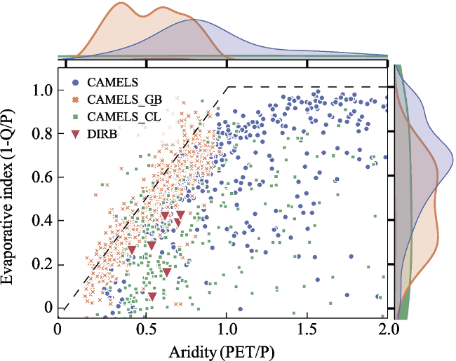
Figure 7 Water balance of the CAMESL, CAMELS_GB, CAMELS_CL, and DIRB catchments depicted within the Budyko scheme, with the right and upper axes showing corresponding variable histograms |
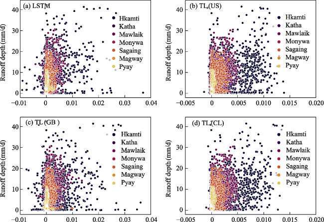
Figure 8 The relationship between runoff depth and integrated gradient (IG) of daily precipitation for Long Short-Term Memory (LSTM) in panel (a), transfer learning from United States (TL(US)) in panel (b), Transfer learning from Great Britain (TL(GB)) in panel (c), and transfer learning from Chile (TL(CL)) in panel (d) across all sub-basins |
Table S1 Summary of the forcing and attribute variables from CAMELS, CAMELS-GB, CAMELS-CL datasets |
| Dataset | Forcing | Static basin attributes | |
|---|---|---|---|
| Variable name | Description | ||
| Data for DIRB | PRCP | Averaged precipitation | lat, lon, altitude, area, soil_bulk_density, p_mean, q_mean |
| T_max | Daily maximum temperature | ||
| T_min | Daily minimum temperature | ||
| CAMELS | PRCP | Averaged precipitation | elev_mean, slope_mean, area_gages2, frac_forest, lai_max, lai_diff, dom_land_cover_frac, dom_land_cover, root_depth_50, oil_depth_statsgo, soil_porosity, soil_conductivity, max_water_content, geol_1st_class, geol_2nd_class, geol_porostiy, geol_permeability, p_mean, pet_mean, p_seasonality, frac_snow, aridity, high_prec_freq, high_prec_dur, low_prec_freq, low_prec_dur.* |
| SRAD | Incident shortwave radiation | ||
| Tmax | Daily maximum temperature | ||
| Tmin | Daily minimum temperature | ||
| Vp | Water vapor pressure | ||
| Dayl | Duration of daylight period | ||
| CAMELS-GB | Precipitation | Averaged precipitation | p_mean, pet_mean, aridity, p_seasonality, discharges, inter_high_perc, q_mean, runoff_ratio, stream_elas, baseflow_index, Q5, Q95, wood_perc, ewood_perc, grass_perc, shrub_perc, crop_perc, urban_perc, inwater_perc, bares_perc, sand_perc, silt_perc, clay_perc, organic_perc, bulkdens, tawc, porosity_cosby, porosity_hypres, conductivity_cosby, conductivity_hypres, root_depth, soil_depth_pelletier, gauge_lat, gauge_lon, gauge_elev, area, dpsbar, elev_mean, elev_min.* |
| Temperature | Averaged temperature | ||
| Humidity | Averaged specific humidity | ||
| Pet | Averaged potential evaporation | ||
| Shortwave_rad | Averaged downward shortwave radiation | ||
| Longwave_rad | Averaged longwave radiation | ||
| Windspeed | Averaged wind speed | ||
| CAMELS-CL | precip_cr2met | Averaged precipitation | area, elev_mean, slope_mean, nested_inner, geol_class_1st_frac, geol_class_2nd_frac, crop_frac, nf_frac, fp_frac, grass_frac, shrub_frac, wet_frac, imp_frac, lc_barren, snow_frac, lc_glacier, fp_nf_index, forest_frac, dom_land_cover_frac, land_cover_missing, p_mean_cr2met, pet_mean, aridity_cr2met, p_seasonality_cr2met, frac_snow_cr2met, high_prec_freq_cr2met, high_prec_dur_cr2met, low_prec_freq_cr2met, low_prec_dur_cr2met, big_dam, p_mean_spread, q_mean, runoff_ratio_cr2met, stream_elas_cr2met, slope_fdc, baseflow_index, hfd_mean, Q95, Q5, high_q_freq, high_q_dur, low_q_freq, low_q_dur, zero_q_freq, sur_rights_n, interv_degree. * |
| tmax | Daily maximum temperature | ||
| tmin | Daily minimum temperature | ||
| swe | Daily snow water equivalent | ||
| pet _8d_modis | Potential evapotranspiration obtained from MODIS | ||
*Because of the long-list of attributes from CAMELS-GB and CAMELS-CL, we refer the readers to their respective publications for explanations of variable names. |
Table S2 Hyperparameter values (chosen/tested) for all models |
| Model* | Length of training instances | LSTM dropout rate | Mini-batching size | LSTM hidden size | Number of training epochs | |
|---|---|---|---|---|---|---|
| LSTM | DIRB | 365/{100, 200, 365} | 0.5/{0, 0.3, 0.5} | 2/{2,5} | 64/{32,64,128} | 250/[100,300] |
| Source model | CAMELS | 100/{50,100,200} | 256/{128,256} | 300/[100,500] | ||
| CAMELS-GB | 128/{64,128,256} | 256/{128,256} | 300/[100,500] | |||
| CAMELS-CL | 128/{64,128,256} | 256/{128,256} | 300/[100,500] | |||
| TL model for DIRB | TL (US)-optimal | 2/{2,5} | 256/256 | 300/[100,300] | ||
| TL (GB)-optimal | 2/{2,5} | 256/256 | 240/[100,300] | |||
| TL (CL)-optimal | 2/{2,5} | 256/256 | 180/[100,300] | |||
* All the models were trained for the five-member ensemble with random seeds. For the tested values, square brackets indicate the range of values tested, while curly braces indicate the discrete values that were tested. Dropout rate is the fraction of connections set to 0 by the dropout operator. Hidden size is the size of g, i, f, t and the associated weight matrices in LSTM. Mini-batch is how many basins are grouped together to calculate the loss function before a gradient update is executed. With an epoch, there are as many forward simulations to run through all data points once. |
Table S3 Summary of the driving data for the MIKE SHE |
| Component | Data type | Source | Time period | Resolution |
|---|---|---|---|---|
| Topography | DEM | ASTER Global Digital Elevation Model v002 | NA | 30 m |
| Meteorology | Precipitation | CHIRPS (https://chc.ucsb.edu/data/chirps) | 1996-2010 | 0.25° |
| Temperature | ERA5-land(https://cds.climate.copernicus.eu/) | 1996-2010 | 0.01° | |
| Vegetation | Land use | MCD12Q1 data (http://www.gscloud.cn/) | 2005 | 500 m |
| Leaf-area index | CLASS (http://www.glass.umd.edu/) | 1996-2010 | 0.05° | |
| Soil | Surface and Sectional type | Harmonized World Soil Database | NA | 1km |
Table S4 Summary of the selected parameters used for the MIKE SHE |
| Component | Parameter | Unit | value | |
|---|---|---|---|---|
| Evapotranspiration | Coefficient, C1 | - | 0.3 | |
| Coefficient, C2 | - | 0.2 | ||
| Coefficient, C3 | mm/day | 20 | ||
| Canopy interception | mm | 0.05 | ||
| Two-layer water balance ET parameter | - | 1 | ||
| Root-density distribution | 1/m | 0.25 | ||
| Snowmelt | Melting temperature | ℃ | 0 | |
| Degree-day coefficient | mm/day/℃ | 1.5 | ||
| Rivers and lakes | Manning coefficient | m1/3/s | 30 | |
| Overland flow | Manning coefficient | m1/3/s | 25 | |
| Detention storage | mm | 0 | ||
| Initial water depth | mm | 0 | ||
| Saturated flow | Interflow reservoir | Specific yield | - | 0.35 |
| Time constant | day | 70 | ||
| Baseflow reservoir 1 | Specific yield | - | 0.3 | |
| Time constant | day | 260 | ||
| Baseflow reservoir 2 | Specific yield | - | 0.3 | |
| Time constant | day | 850 | ||
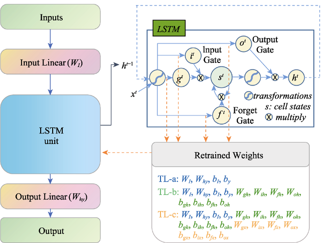
Figure S1 The architecture of transfer learning (TL) and weight freezing strategies of TL-a, TL-b and TL-c |
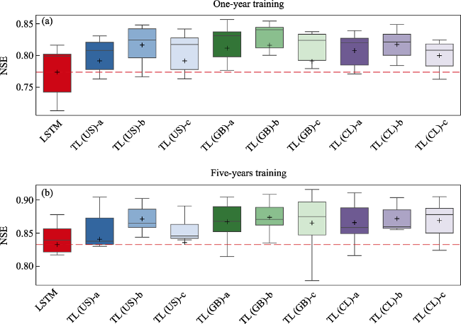
Figure S2 NSE values for the mean discharge from a five-member ensemble, corresponding to the local LSTM and TLs with different weight freezing strategy in data deficit scenario (1-year training) and normal training (five-years training) |
| [1] |
|
| [2] |
|
| [3] |
|
| [4] |
|
| [5] |
|
| [6] |
|
| [7] |
|
| [8] |
|
| [9] |
|
| [10] |
|
| [11] |
|
| [12] |
|
| [13] |
|
| [14] |
|
| [15] |
|
| [16] |
|
| [17] |
|
| [18] |
|
| [19] |
|
| [20] |
|
| [21] |
|
| [22] |
|
| [23] |
|
| [24] |
|
| [25] |
|
| [26] |
|
| [27] |
|
| [28] |
|
| [29] |
|
| [30] |
|
| [31] |
|
| [32] |
|
| [33] |
|
| [34] |
|
| [35] |
|
| [36] |
|
| [37] |
|
| [38] |
|
| [39] |
National Water Resources Committee (NWRC), 2018. The Ayeyarwady State of the Basin Assessment. SOBA 1.2: Surface Water Resources. National Water Resources Committee.
|
| [40] |
|
| [41] |
|
| [42] |
|
| [43] |
|
| [44] |
|
| [45] |
|
| [46] |
|
| [47] |
|
| [48] |
|
| [49] |
|
| [50] |
|
| [51] |
|
| [52] |
|
| [53] |
The United Nations World Water Development Report 2020: Water and Climate Change, 2020. UNESCO.
|
| [54] |
The United Nations World Water Development Report 2021: Valuing Water, 2021. UNESCO.
|
| [55] |
|
| [56] |
|
| [57] |
|
| [58] |
|
| [59] |
|
| [60] |
|
| [61] |
|
/
| 〈 |
|
〉 |