Research Articles

Spatial scaling effects of gully erosion in response to driving factors in southern China

  • LIU Zheng ,
  • WEI Yujie , * ,
  • CUI Tingting ,
  • LU Hao ,
  • CAI Chongfa
Expand
  • College of Resources and Environment, Huazhong Agricultural University, Wuhan 430070, China
*Wei Yujie (1988-), Associate Professor, E-mail:

Liu Zheng (1994-), PhD Candidate, specialized in soil erosion and gully susceptibility assessment. E-mail:

Received date: 2023-08-02

  Accepted date: 2024-02-07

  Online published: 2024-05-31

Supported by

National Natural Science Foundation of China(42277329)

National Natural Science Foundation of China(41807065)

National Natural Science Foundation of China(42077067)

China Postdoctoral Science Foundation(2018M640714)

Fundamental Research Funds for the Central Universities(2662021ZHQD003)

Abstract

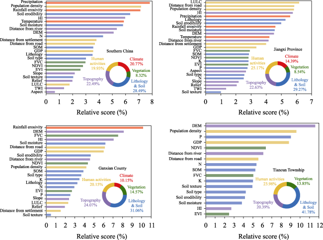
Gully erosion, an integrated result of various social and environmental factors, is a severe problem for sustainable development and ecology security in southern China. Currently, the dominant driving forces on gully distribution are shown to vary at different spatial scales. However, few systematic studies have been performed on spatial scaling effects in identifying driving forces for gully erosion. In this study, we quantitatively identified the determinants of gully distribution and their relative importance at four different spatial scales (southern China, Jiangxi province, Ganxian county, and Tiancun township, respectively) based on the Boruta algorithm. The optimal performance of gully susceptibility mapping was investigated by comparing the performance of the multinomial logistic regression (MLR), logistic model tree (LMT), and random forest (RF). Across the four spatial scales, the total contributions of gully determinants were classified as lithology and soil (32.65%) > topography (22.40%) > human activities (22.31%) > climate (11.32%) > vegetation (11.31%). Among these factors, precipitation (7.82%), land use and land cover (6.16%), rainfall erosivity (10.15%), and elevation (11.59%) were shown to be the predominant factors for gully erosion at the individual scale of southern China, province, county, and township, respectively. In addition, contrary to climatic factors, the relative importance of soil properties and vegetation increased with the decrease of spatial scale. Moreover, the RF model outperformed MLR and LMT at all the investigated spatial scales. This study provided a reference for factor selection in gully susceptibility modeling and facilitated the development of gully erosion management strategies suitable for different spatial scales.

Cite this article

LIU Zheng , WEI Yujie , CUI Tingting , LU Hao , CAI Chongfa . Spatial scaling effects of gully erosion in response to driving factors in southern China[J]. Journal of Geographical Sciences, 2024 , 34(5) : 942 -962 . DOI: 10.1007/s11442-024-2234-y

1 Introduction

Gully erosion, the advanced stage of soil erosion, is defined as a channel that cannot be eliminated by normal tillage operations (Poesen et al., 2003; Amiri et al., 2019). Globally, gully erosion contributed 10%-94% of the total sediment yield, so it has been regarded as the primary source of soil loss, especially in hilly and mountainous areas (Zabihi et al., 2016). Meanwhile, the widespread on- and off-site effects of gully erosion pose an enormous threat to land degradation and ecosystem services, such as depleting soil quality, decreasing crop yields, declining biomass production rates, and destroying roads and buildings (Poesen, 2018). In the past several decades, gully erosion has been recognized as a national issue in the hilly areas of southern China (Figure 1) due to its complex formation mechanism, sudden occurrence, and severe threat to the ecological system (Wei et al., 2021b). Although a series of ecological restoration projects have been implemented (Zhang et al., 2021), more than 2.39 × 10⁵ gullies are still distributed in southern China (Zhong et al., 2013). The less effective control of gully erosion is mainly attributed to the ambiguous contribution of influential factors, especially the variation of gully erosion determinants at various spatial scales (Zhou et al., 2023).
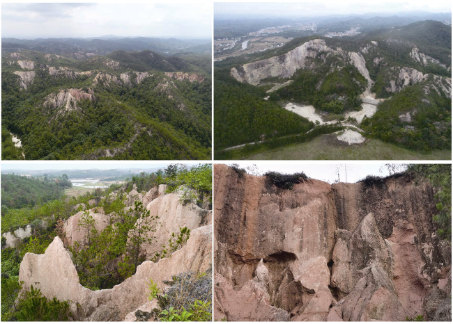
Figure 1 Typical gully landforms in southern China
Gully erosion formation and development are controlled by geomorphological evolution and human activities (Gayen et al., 2019). According to existing studies, gully erosion has an obvious scale effect process, and the driving factors vary significantly between different spatial scales (Borrelli et al., 2020). For instance, soil texture, soil organic matter, soil moisture, soil organic carbon, coarse fragment content and cover, soil depth, and bulk density have been widely accepted as the most relevant indicators at the plot scale (Kheir et al., 2008; Castillo and Gomez, 2016). Topographic variables (e.g., elevation, slope gradient, and slope aspect) can provide enough energy for gully initiation and expansion, which are critical at the watershed scale (Jaafari et al., 2022). Climate, particularly rainfall, is a dominant driver at the regional scale, with triggering and conditioning effects on gully erosion (Sun et al., 2013; Vanmaercke et al., 2016). However, previous studies on the influencing factors of gully erosion were mainly concentrated on a specific scale, i.e., watershed (Rahmati et al., 2017), province (Liao et al., 2019), or region (Lana et al., 2022), and regional differences of gully erosion in different areas make it difficult to identify of spatial scale effects on gully determinants (Wei et al., 2022). This suggested that a systematical study on the scaling effects of driving factors on a specific type of gully erosion could facilitate a better understanding of gully erosion mechanism (Wang et al., 2018).
With the increasing requirement for modeling erosion processes, downscaling or upscaling methodologies, and decision-making, spatial scale effects have become a hot topic worldwide (Vanmaercke et al., 2021), due to the variation of the relative importance of influential factors with the changes of spatial scales (Descroix et al., 2008). Additionally, gully erosion research is shifting from the slope/plot, small watershed/local/township, watershed/state/regional scale to national/global scale (Liu et al., 2021), and the scaling effect plays a critical role in these transitions (Zabihi et al., 2018). Previous studies have also shown that the spatial scale effect is primarily limited by the complexity of erosion processes and the heterogeneity of drivers (Peeters et al., 2008). Good coordination between influential factors should be ensured at different spatial scales (Fu et al., 2006), but the standard guidelines for factor selection are still being debated, which could directly affect the outcome of prediction modeling (Mokarram and Zarei, 2021). Therefore, research efforts should be devoted to selecting appropriate indices and comprehensively comparing the relative importance of the driving factors to gully erosion at different spatial scales to reveal the scale dependence of gully erosion.
To better prevent gully erosion, gully susceptibility modeling has gained increasing attraction in recent decades (Arabameri et al., 2020). Globally, several Geographic Information System (GIS)-based bivariate models were shown to be beneficial for accurate assessment of gully erosion susceptibility (Azareh et al., 2019). In recent years, many methods have been developed, including traditional statistical models (e.g., logistic regression, information value, frequency ratio, certainty factors, conditional probability, weight of evidence, and evidential belief) and machine learning models (such as random forest, logistic model tree, support vector machines, and artificial neural network) (Wang et al., 2022). These techniques have also been widely applied to risk modeling of other environmental elements such as landslides (Ngo et al., 2021), floods (Khosravi et al., 2018), and groundwater (Chen et al., 2018). Although the traditional statistical model and machine learning methods have their strengths (Micheletti et al., 2013), it is still necessary to identify the optimal model at a specific spatial scale to meet the increasing requirement for an accurate assessment of potential vulnerability (Song et al., 2016). This may be achieved by cross-comparison of different categories of models (Wei et al., 2021a). Currently, limited information is available on the optimal methods for gully susceptibility modeling at different spatial scales.
Therefore, this study investigated the scaling effects in driving factor identification for gully erosion at the scales of southern China, province, county, and township in terms of natural and artificial factors. The main objectives were (1) to identify the differentiation of driving factors on gully erosion at four different spatial scales using the Boruta algorithm, (2) to evaluate the performance of multinomial logistic regression, logistic model tree, and random forest on gully susceptibility modeling at various spatial scales, and (3) to determine the gully-prone areas by mapping the spatial distribution of gully erosion susceptibility. The results may contribute to a better understanding of the scale effect on gully erosion and facilitate decision-making for effective gully erosion management strategies at various spatial scales.

2 Materials and methods

2.1 Study area

Four watersheds with different spatial scales in the granitic hill region of southern China were selected as the study areas (Figure 2), including southern China (20°13′-34°38′N and 104°28′-120°40′E), Jiangxi province (24°29-30°05′N and 113°34′-118°29′E), Ganxian county (25°26′-26°17′N and 114°42′-115°22′E) in Jiangxi province, and Tiancun township (26°04′-26°14′N and 115°02′-115°16′E) in Ganxian county, Jiangxi province. The four sites were the focus-study areas of gully erosion (Wei et al., 2021b) due to the high density, various sizes, and different development stages of gullies (2005 National Survey by the Yangtze River Water Resources Commission of the Ministry of Water Resources of China), suggesting the four sites can provide an ideal place for analyzing the spatial scale effects of gully erosion.
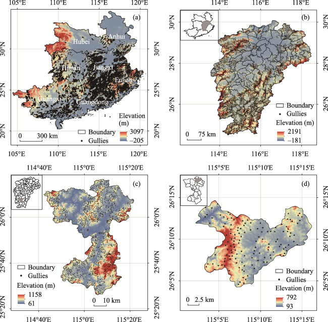
Figure 2 Location of the study area (a. southern China; b. Jiangxi province; c. Ganxian county; d. Tiancun township)
There are 239125, 48058, 4138, and 590 gullies in southern China, Jiangxi province, Ganxian county, and Tiancun township, respectively. These areas have a subtropical monsoon climate, favoring the accumulation of weathering materials (Xia et al., 2019). The granite weathering crust thickness ranges from 5 to 70 m, providing a material basis for gully development (Liao et al., 2019). The primary lithology is granite (syenite), especially the syenite and monzogranite, and the granite in these areas was formed mainly in the Early Caledonian and the Yanshan periods, with weathered granitic acidic red soil as the primary soil type. Field investigation found that most gullies are located in low mountains or hills with an old geological stage (Wei et al., 2022). The natural vegetation is evergreen broadleaf forest, and gully initiation was triggered by large-scale forest destruction (Woo et al., 1997). Pinus massoniana, Eriachne pallescens, Phragmites australis, and Dicranopteris linearis are the main tree species in the gully areas. Detailed characteristics of these areas are given in Table 1.
Table 1 Detailed characteristics of the study area in southern China
Site Latitude/longitude Area
(km2)
Elevation
(m)
Mean annual
temperature
(℃)
Mean annual
precipitation (mm)
Gullies Gully area
(km2)
Southern China 20°13′-34°38′N, 104°28′-120°40′E 1,241,500 -205-3097 14-24 754.5-2312.3 23,9125 1220
Jiangxi province 24°29′-30°05′N, 113°34′-118°29′E 166,900 -181-2191 16.3-19.5 1341-1943 48,058 207.40
Ganxian county 25°26′-26°17′N, 114°42′-115°22′E 2993.09 61-1158 16.3-20.5 1600.5-1700 4138 18.1
Tiancun township 26°04′-26°14′N, 115°02′-115°16′E 222.21 93-792 17.2-19.8 1622.8-1682.1 590 1.69

2.2 Methodology

The methodology in the four different spatial scales of watershed consists of five steps (Figure 3): (1) preparing the gully inventory map; (2) extracting the geo-environmental factors; (3) analyzing the multicollinearity between gully susceptibility and potential conditions; (4) assessing the driving factors of gully erosion at four different scales; (5) modeling and mapping gully erosion susceptibility.
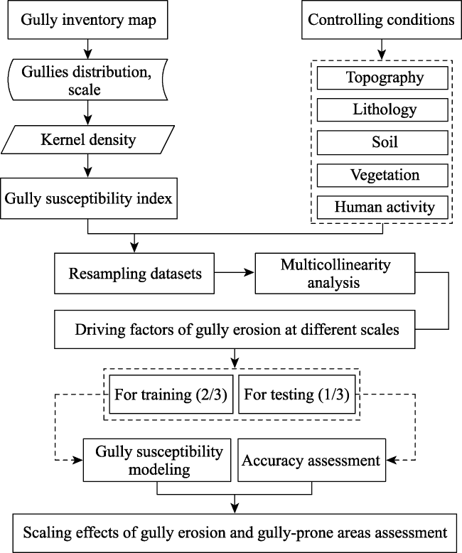
Figure 3 Flowchart of methodology in this study

2.2.1 Gully inventory mapping

The gully inventory was collected from the National Survey on Soil and Water Loss organized by the Ministry of Water Resources of China (Yangtze River Water Conservancy Commission) in 2005. The number, size, and distribution of gullies were validated and supplemented by field survey and visual interpretation of WorldView-2 commercial satellite imagery with a high spatial resolution of 0.5 m acquired in November 2018. For gully inventory mapping, the points and areas of gullies were taken as the input element; the search radius was 5 km, 3 km, 2 km, and 1 km, from southern China to Tiancun township, respectively; the output pixel size was 30 m. Finally, the gully susceptibility index (GSI) was calculated using the kernel density analysis (Kropat et al., 2015) in ArcGIS 10.2, with equations 1-2:
$GSI\left( x \right)=\underset{i=1}{\overset{n}{\mathop \sum }}\,\frac{1}{nh}k\left( \frac{x-{{x}_{i}}}{h} \right)$
$k\left( x \right)=\left\{ \begin{matrix} ~~3{{\text{ }\!\!\pi\!\!\text{ }}^{-1}}{{\left( 1-{{x}^{T}}x \right)}^{2}}\text{if }{{x}^{T}}x<1 \\ 0\ \text{ otherwise} \\\end{matrix} \right.$
where n is the number of element points with a distance less than or equal to h from x; h, the search radius; xi, the ith data point; k(x), the kernel function. The gully susceptibility index (GSI) dataset was divided by Natural Breaks into four classes (1 to 4): very low, low, moderate, and high susceptibility.
To create the sampling dataset, 31,569, 4459, 420, and 148 small watersheds were divided using hydrological analysis in ArcGIS 10.2. The number of pixels in the catchment area was 10,000, 8000, 2000, and 1000, and the mean sizes of sub-catchments were 10 km2, 8 km2, 3 km2, and 1.5 km2. In addition, 239,125, 48,058, 4138, and 590 points were randomly generated by Hawth’s tools in non-gully sub-catchments. Finally, gully points (gully areas) and random points (non-gully areas) were combined into the sampling dataset, with two-thirds of the sampling dataset used for training and one-third for testing.

2.2.2 Selection of potential geo-environmental factors

Gully erosion is influenced by various factors (Valentin et al., 2005), and gully occurrence and dynamics have been shown to be influenced by more than 100 practical factors, including topography, soils and lithology, climate and weather, vegetation cover, and human activities (Poesen et al., 2003). Additionally, previous studies have mentioned that insignificant and unavailable influencing factors should be excluded from consideration (Conoscenti et al., 2013). Moreover, weak spatial heterogeneity of homogeneous conditions had little effect on gully erosion (Zhang et al., 2022). This indicated that factor selection at multiple scales is more complex than at a single scale (Sonneveld et al., 2005), so it is necessary to comprehensively consider the input of controlling factors and their pixel sizes according to the study area, data availability, and research objectives (Drăguţ et al., 2009). Based on the literature review, 27 geo-environmental factors were considered in this study, including lithology and soil (Chen et al., 2018), topography (Liao et al., 2019), climate (Hayas et al., 2019), vegetation (Wei et al., 2021a), and human activities (Frankl et al., 2018) (Table 2).
Table 2 Conditioning factors of gully erosion
Factor Time resolution Data description Data source
Lithology 2007 Raster; 1:500,000 (https://geocloud.cgs.gov.cn/)
Soil type 2000 Raster; 1:1,000,000 (http://www.resdc.cn)
Soil erodibility 2018 Raster; 30 m×30 m http://www.geodata.cn
Soil texture 2018 Raster; 30 m×30 m (http://www.resdc.cn)
Soil moisture (m³/m³) 2018.05 Raster; 100 m×100 m (http://www.resdc.cn)
N (g/kg) 2018 Raster; 90 m×90 m http://www.geodata.cn
P (g/kg) 2018 Raster; 90 m×90 m http://www.geodata.cn
K (g/kg) 2018 Raster; 90 m×90 m http://www.geodata.cn
SOM (g/kg) 2018 Raster; 90 m×90 m http://www.geodata.cn
Elevation (m) 2019 Raster; 30 m×30 m (http://www.geodata.cn)
Slope (°) 2019 Raster; 30 m×30 m (http://www.geodata.cn)
Aspect 2019 Raster; 30 m×30 m (http://www.geodata.cn)
Relief 2019 Raster; 30 m×30 m (http://www.geodata.cn)
TWI 2019 Raster; 30 m×30 m (http://www.geodata.cn)
HI 2019 Raster; 30 m×30 m (http://www.geodata.cn)
River 2018 Vector (line); 1000 m×1000 m (http://www.resdc.cn)
Temperature (℃) 1991-2020 Raster; 30 m×30 m (http://digitalmountain.imde.ac.cn/)
Rainfall erosivity (MJ·mm/(ha·h·a)) 1991-2020 Raster; 30 m×30 m (http://digitalmountain.imde.ac.cn/)
Precipitation (mm) 1991-2020 Raster; 30 m×30 m (http://digitalmountain.imde.ac.cn/)
FVC 2018.05 Raster; 500 m×500 m (http://ladsweb.modaps.eosdis.nasa.gov/)
EVI 2018.05 Raster; 250 m×250 m (http://ladsweb.modaps.eosdis.nasa.gov/)
NDVI 2018.05 Raster; 500 m×500 m (http://ladsweb.modaps.eosdis.nasa.gov/)
Population density (person/km2) 2018 Raster; 30 m×30 m (http://www.resdc.cn)
GDP (yuan/km2) 2018 Raster; 30 m×30 m (http://www.resdc.cn)
LULC 2018 Raster; 30 m×30 m (http://www.resdc.cn)
Road 2018 Vector (line); 1:1,000,000 (http://www.resdc.cn)
Settlement 2018 Vector (point); 1:1,000,000 (http://www.resdc.cn)

Note: N, total nitrogen; P, total phosphorus; K, total kalium; SOM, soil organic matter; TWI, topographic wetness index; HI, hypsometric integral; NDVI, normalized difference vegetation index; FVC, fraction vegetation coverage; EVI, enhanced vegetation index; GDP, gross domestic product; LULC, land use and land cover.

Moreover, the pixel resolution of these potential drivers was appropriate for each of our study sites (Hengl, 2006). Furthermore, two quantitative steps (multicollinearity analysis and importance ranking by the Boruta algorithm) were adopted during factor elimination, thereby reducing human error and uncertainty (Wei et al., 2022).
For consistency of calculation and processing, all geo-environmental factors were resampled to 30 m pixel resolution, and the attribute values of continuous and categorical variables were merged into the resampled dataset using extract values to points function in ArcGIS 10.2. A detailed description of the conditioning factors used in this study is shown in Table 2.

2.3 Methods

2.3.1 Multicollinearity analysis

Eliminating highly multicollinear variables is a technical way to prevent model accuracy reduction (Achour and Pourghasemi, 2020). Tolerance and variance inflation factor (VIF), which were regarded as high-efficiency indexes to test the multicollinearity problem (Amiri et al., 2019), were calculated using SPSS V. 20 with equations 3 and 4:
$Tolerance=1-{{R}_{i}}^{2}$
$VIF=\left[ \frac{1}{Tolerance} \right]$
where Ri2 is the determination coefficient. No multicollinearity occurred with tolerance > 0.10 or VIF < 10. Herein, multicollinearity problems were observed in southern China, Ganxian county, and Tiancun township, excluding Jiangxi province. Due to severe multicollinearity, factor elimination was performed for P and K (in southern China), temperature and precipitation (in Ganxian county), temperature, rainfall erosivity, and precipitation (in Tiancun township) (Table 3).
Table 3 Factor elimination using multicollinearity analysis and Boruta algorithm
Factors Southern China Province County Township
VIF Decision VIF Decision VIF Decision VIF Decision
Lithology 1.097 Confirmed 2.497 Confirmed 1.292 Confirmed 3.545 Reject
Soil type 1.012 Confirmed 1.095 Confirmed 1.337 Confirmed 3.267 Confirmed
Soil erodibility 1.427 Confirmed 1.819 Confirmed 1.326 Confirmed 1.718 Confirmed
Soil texture 1.199 Confirmed 1.188 Confirmed 1.172 Confirmed 3.004 Confirmed
Soil moisture (m3/m3) 2.206 Confirmed 1.268 Confirmed 1.180 Confirmed 3.862 Confirmed
N (g/kg) 6.609 Confirmed 6.299 Confirmed 3.533 Confirmed 4.116 Confirmed
P (g/kg) 13.48 / 1.083 Confirmed 1.644 Confirmed 6.537 Confirmed
K (g/kg) 13.354 / 1.448 Confirmed 2.557 Confirmed 8.480 Confirmed
SOM (g/kg) 8.144 Confirmed 9.691 Confirmed 5.466 Confirmed 5.291 Confirmed
Elevation (m) 4.278 Confirmed 6.522 Confirmed 8.989 Confirmed 7.803 Confirmed
Slope (°) 5.863 Confirmed 6.575 Confirmed 4.486 Confirmed 5.163 Reject
Aspect 1.002 Confirmed 1.407 Confirmed 1.032 Reject 1.140 Reject
Relief 5.733 Confirmed 6.566 Confirmed 4.623 Confirmed 5.239 Reject
TWI 1.095 Confirmed 1.087 Confirmed 1.157 Reject 1.278 Reject
HI 1.468 Confirmed 1.171 Confirmed 1.483 Confirmed 1.853 Confirmed
Distance from river (m) 1.052 Confirmed 1.089 Confirmed 1.296 Confirmed 1.930 Confirmed
Temperature (℃) 3.938 Confirmed 2.833 Confirmed 41.837 / 208.540 /
Rainfall erosivity (MJ·mm/(ha·h·a)) 4.297 Confirmed 2.854 Confirmed 1.818 Confirmed 35.281 /
Precipitation (mm) 3.415 Confirmed 1.920 Confirmed 25.103 / 170.030 /
FVC 4.062 Confirmed 4.858 Confirmed 4.177 Confirmed 3.224 Confirmed
EVI 1.427 Confirmed 1.761 Confirmed 1.266 Confirmed 1.663 Reject
NDVI 3.422 Confirmed 4.526 Confirmed 3.818 Confirmed 3.007 Confirmed
Population density (person/km2) 1.822 Confirmed 2.032 Confirmed 1.253 Confirmed 1.925 Confirmed
GDP (yuan/km2) 1.732 Confirmed 1.761 Confirmed 1.289 Confirmed 2.021 Confirmed
LULC 1.411 Confirmed 3.615 Confirmed 1.103 Confirmed 1.276 Reject
Distance from road (m) 1.428 Confirmed 1.471 Confirmed 1.425 Confirmed 4.565 Confirmed
Distance from settlement (m) 1.234 Confirmed 1.205 Confirmed 1.261 Confirmed 1.215 Reject

Note: When VIF > 10, the factor is immediately eliminated and does not participate in the second screening by the Boruta algorithm. The decision was calculated by the Boruta algorithm, with Confirmed for importance, and Reject for unimportance and inconsideration.

2.3.2 Boruta algorithm

The Boruta algorithm, a feature selection algorithm created by the random forest classification in the R statistical package (Amiri et al., 2019), is a self-sampling ensemble where the degree of importance is determined by decision tree voting (Kursa and Rudnicki, 2010). Compared to other feature selection algorithms, the Boruta algorithm can not only eliminate insignificant factors, but also can rank the contribution of significant geo-environmental factors to gully erosion susceptibility (Kursa and Rudnicki, 2010). In this study, two elements (aspect and TWI) in Ganxian county and seven factors (lithology, slope, aspect, relief, TWI, LULC, and distance from settlement) in Tiancun township were rejected (Table 3), so 25, 27, 23, and 17 geo-environmental factors could significantly influence gully erosion and were selected as input variables.

2.4 Gully erosion susceptibility modeling

2.4.1 Multinomial logistic regression

Multinomial logistic regression (MLR) is a powerful linear statistical technique widely used to calculate the relationship between the dependent binary variable and a set of independent variables (Chaplot et al., 2005). The predicted result was generally understood as a membership probability event (Lucà et al., 2011). This model aims to define the quantitative relationship between gully susceptibility index and causal elements. The probability of an event occurring could be represented equations 5 and 6:
$p=\frac{1}{\left( 1+ex{{p}^{-z}} \right)}$
$z={{b}_{0}}+{{b}_{1}}{{x}_{1}}+{{b}_{2}}{{x}_{2}}+\cdots +{{b}_{n}}{{x}_{n}}$
where p represents the likelihood of gully erosion (scoping of 0 to 1); z, the linear combination of variables (ranging from -∞ to +∞); b0, intercept; bi, coefficient; xi, independent variables.

2.4.2 Logistic model tree

Logistic model tree (LMT) is non-linear with a combination of logistic regression and decision tree proposed by Landwehr (2003). This model has been widely used to process mass data with the advantages of few parameters, short-time consumption, and high accuracy (Arabameri et al., 2020). In this model, the logit boost algorithm was used to construct the logistic regression function on the tree nodes and the CART method was adopted for pruning to prevent overfitting (Kadavi et al., 2019). The posterior probability of each leaf node can be expressed by linear logistic regression with equation 7.
${{P}_{j}}\left( x \right)=\frac{{{e}^{{{F}_{j}}\left( x \right)}}}{\mathop{\sum }_{k=1}^{j}{{e}^{{{F}_{j}}\left( x \right)}}}$
where Fj(x) indicates the linear regression function, and j represents the number of classes.

2.4.3 Random forest

Random forest (RF) is a highly accurate ensemble learning proposed by Breiman (2001), and the bagging algorithm has been widely used in gully erosion susceptibility modeling (Pourghasemi and Rahmati, 2018). The basic idea is that multiple independent decision trees were built using the out-of-bag bootstrap strategy, followed by combining the prediction results of each decision tree, and determining the final model precision by decision tree voting (Liaw and Wiener, 2002). In this study, each decision tree and feature were randomly selected to increase the modeling accuracy, and the modeling process was run in R 3.5.1 software using the “random forest” package.

2.5 Model validation

The receiver operating characteristic (ROC) curve and accuracy were employed to validate the performance of the models. The ROC is a graph established by sensitivity and 1-specificity with different cut-off thresholds on other susceptibility classes, where a high area under the ROC curve (AUC) can reflect a high goodness of fit and model consistency (Zabihi et al., 2018). In addition, the accuracy, ranging from 0 to 1, can show the model’s overall performance (Bui et al., 2016). These procedures were run in the R 3.5.1 environment using the “pROC” and “caret” packages. The accuracy can be described by equation 8:
$Accuracy=\frac{TP+TN}{TP+TN+FP+FN}$
where TP, TN, FP, and FN represent true positive, true negative, false positive, and false negative, respectively.

3 Results

3.1 Scale effects on driving factors for gully erosion

In Figure 4, the relative importance of the driving factors was seen to vary significantly at the four investigated spatial scales. According to the classification of the potential factors, the average contribution values were ranked in the order of lithology and soil (32.65%) > topography (22.40%) > human activities (22.31%) > climate (11.32%) > vegetation (11.31%) across the four spatial scales. Among these factors, lithology and soil properties dominated gully erosion at the scales of southern China, province, county, and township, and their contribution to gully erosion at these four scales was 28.49%, 29.27%, 31.06%, and 41.78%, respectively, indicating an emphasized impact of lithology and soil properties on gully erosion as spatial scale decreased. Similarly, vegetation was more critical at the scale of county (14.57%) and township (13.85%) than at the scale of southern China (8.32%) and province (8.54%). In contrast, the contributions of climatic factors showed a downtrend and were most important in the scale of southern China (20.77%). Moreover, with decreasing spatial scale, the contribution of topography to gully erosion followed a trend of increasing first and then decreasing, with its peak at the county scale (24.07%). The total contribution of human activities showed an N-shaped variation, with the highest value in the province scale (25.17%) and the smallest value in the scale of southern China (19.93%).
Figure 4 Analysis of the importance of variables using the Boruta algorithm (N, total nitrogen; P, total phosphorus; K, total kalium; SOM, soil organic matter; TWI, topographic wetness index; HI, hypsometric integral; NDVI, normalized difference vegetation index; FVC, fraction vegetation coverage; EVI, enhanced vegetation index; GDP, gross domestic product; LULC, land use and land cover; DEM, elevation)
The relative importance of a single factor suggested that precipitation (7.82%), land use and land cover (LULC) (6.16%), rainfall erosivity (10.15%), and elevation (DEM) (11.59%) were the most critical factors for triggering gully erosion at the individual scale of southern China, province, county, and township, respectively (Figure 4). In addition, elevation (7.33%), population density (6.69%), rainfall erosivity (5.46%), gross domestic product (GDP) (5.43%), hypsometric integral (HI) (5.37%), distance from road (5.31%), and soil moisture (5.09%) were the top seven leading factors at all the four scales based on their average contribution values. Notably, with decreasing basin scale, the relative importance increased for DEM and GDP, but decreased for precipitation and rainfall erosivity. Meanwhile, the relative importance exhibited a trend of increasing first and then decreasing for LULC, HI, and distance from road, a V-shaped variation pattern for population density, and an inverse N-shaped trend for rainfall erosivity and soil moisture. Collectively, with the decrease of basin scale, the impact weakens for climate factors, but enhances for soil properties and vegetation.

3.2 Model construction and performance evaluation

The area under receiver operating characteristic curves (AUC-ROC) was used to evaluate the performance of gully erosion susceptibility modeling, and gully susceptibility was further divided into four classes: very low, low, moderate, and high (Figures 5a-5l). In the three models, the RF model was shown to have the highest AUC value in predicting gully erosion susceptibility at each scale, fluctuating between 0.978 and 0.70, followed by the LMT model with its AUC averaging 0.925, 0.898, 0.740, and 0.687, respectively. The MLR model had the lowest mean AUC values (0.827-0.60), especially in the low and medium classes. In Figure 6, the total accuracy of models was also shown to decrease with decreasing spatial scale and data input. Moreover, the RF model was seen to have consistently higher accuracy values than the other two models, keeping pace with the AUC-ROC. Overall, in the three models, the RF model exhibited the highest accuracy in predicting gully erosion susceptibility at different spatial scales.
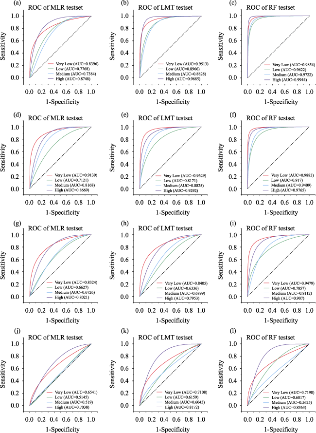
Figure 5 ROC curves of gully susceptibility maps by MLR, LMT, and RF models in different spatial scales (a-c. southern China; d-f. Jiangxi province; g-i. Ganxian county; j-l. Tiancun township)
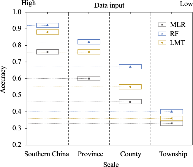
Figure 6 Comparison of model accuracy in terms of scale and data input

3.3 Gully erosion susceptibility assessment

Gully erosion susceptibility was mapped using the RF model (Figures 7a-7d). The very low, low, moderate, and high groups accounted for 61.68%, 27.97%, 7.10%, and 3.25% in southern China, respectively. Notably, the south side (e.g., the center of Guangdong province, north of Jiangxi province, north and east of Guangxi, south of Fujian province, and center and southeast Hunan province) were more susceptible to gully erosion than the northern areas (e.g., Anhui province, Hubei province, and north of Hunan province). In Jiangxi province, gully erosion was concentrated in the north, (especially in the counties of Ganxian, Xingguo, Yudu, and Ningdu), with a susceptibility value of 33.08%, 21.84%, 19.08%, and 26.00% for the very low, low, moderate, and high groups, respectively. At the two smaller spatial scales, the very low, low, moderate, and high groups accounted for 21.89%, 15.71%, 29.56%, and 32.84% in Ganxian county, while 4.38%, 22.42%, 27.66%, and 45.54% in Tiancun township.
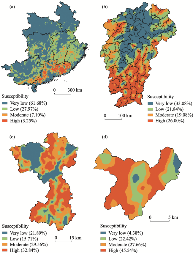
Figure 7 Gully erosion susceptibility maps using the random forest (RF) model (a. southern China; b. Jiangxi province; c. Ganxian county; d. Tiancun township)

4 Discussion

4.1 Scale effect of conditioning factors on gully erosion

Scale, a hot topic in soil erosion, ecology, hydrology and other disciplines, is critical for measuring geographic phenomena (Vanmaercke et al., 2021). A scale effect occurs with the change of a given temporal or spatial scale, which is primarily limited by the complexity of erosion process, the heterogeneity of environments, and the size of monitored research areas (Peeters et al., 2008; Borrelli et al., 2020). The gully distribution with a spatial clustering pattern is non-uniform, suggesting that gully erosion has an apparent scale effect and is susceptible to environmental conditions (Wang et al., 2020). However, the standard guidelines for feature selection are controversial, especially regarding scale transformation (Bui et al., 2016). Additionally, the driving factors of gully erosion vary from case to case (Conforti et al., 2011). Therefore, determining the driving factors of gully erosion and examining their spatial scaling effect is extremely important (Conoscenti et al., 2013). In this study, we found lithology and soil properties as the characteristics most responsible for gully erosion (Figure 4). Previous studies have shown that lithology plays a crucial role in gully distribution, development size, and evolution process (Bernatek-Jakiel and Poesen, 2018). Especially the granite weathering crust thickness was considered as a material basis for gully initiation, which has been confirmed by similar erosion landforms worldwide, such as “Lavaka” in Madagascar (Cox et al., 2010), “Vocorocas” in Brazil (Bezerra et al., 2020), and “Calanchi” in Italy (Caraballo-Arias et al., 2014). Besides, soil physiochemical properties can determine gully occurrence and development by mainly affecting erodibility and hydrological function (Xia et al., 2019). Several field studies demonstrated a significant difference in soil properties along the granite soil profile due to varying weathering degree (Deng et al., 2020; Wei et al., 2021b). Once the soil layer has been eroded, the lower layers have low shear strength and are susceptible to collapsing (Tao et al., 2017).
Human activities can directly trigger gully formation (Borrelli et al., 2020). Our results showed that human activities are also a crucial determinant for gully development at all scales (Figure 4). For example, the LULC ranked first at the province scale, agreeing with the reports of Chen et al. (2019) and Zhou et al. (2021) that unreasonable land use type could influence soil quality, runoff yield, and soil loss rate. Previous studies also indicated that large-scale forest destruction could decrease vegetation cover, cause rapid topsoil loss, expose weathering crust, and trigger gully formation (Woo et al., 1997). Additionally, long-term agricultural activity on slope cropland could affect soil degradation and cause gully occurrence in southern China (Wang et al., 2017). Moreover, the distance from road could significantly affect gully formation, aligning with the conclusion of Arabameri et al. (2018). From the perspective of physical process, road building in hills and mountains can directly generate a steep slope and significantly increase the susceptibility to slope failure, especially during heavy rains (Nyssen et al., 2002). Furthermore, population density ranked top three for gully occurrence at one or more scales, consistent with the conclusions of other researchers (Yuan et al., 2019; Wei et al., 2022). However, Tarolli and Sofia (2016) mentioned that direct evidence for population impact on the gully initiation could hardly be obtained, indicating an uncertain relationship between gully erosion and human activities. Therefore, great attention should be paid to identifying the quantitative impact of human activities on gully erosion.
We also found that the relative importance of other driving factors varies at different spatial scales. For instance, climatic factors showed a downtrend with decreasing spatial scale. It is fascinating to point out that the contribution of precipitation ranked first in southern China and then decreased with declining spatial scales, which may be related to the weak spatial heterogeneity (Zhang et al., 2022). In contrast, with decreasing spatial scales, the importance of elevation rose to the top ranking at the township scale. Lin et al. (2015) confirmed that elevation as a critical factor in the watershed scale, providing sufficient energy for gully initiation and expansion. In addition, elevation change is more drastic at a relatively small scale than at a larger scale, leading to a stronger scouring velocity (Wei et al., 2022). However, the resolution of digital elevation images could directly affect the accuracy of capturing spatial variability in geomorphic processes (Millares et al., 2012). Analogously, vegetation factors, especially NDVI, presented an upward trend with decreasing basin scale. Erktan et al. (2016) reported that vegetation growth and distribution in a smaller spatial scale are more sensitive to climate, topography, and human activities (e.g., agricultural cultivation, deforestation, and urbanization), which can significantly affect the protective effect of vegetation on soil and water. Furthermore, the control effect of soil properties increases with decreasing spatial scale, further supporting the widespread agreement that soil properties are the intrinsic and most important indicators at the plot scale (Castillo and Gomez, 2016). For the increasing importance of soil properties on gully erosion with reducing spatial scale, one possible explanation is that vertical differentiation of soil properties is more likely to cause collapse instability at a relatively small scale than at a larger scale (Liao et al., 2022). Although their correlation with gully erosion could be affected by field sampling accuracy of soil properties (Wu et al., 2021), our results could provide a reference for selecting potential factors to gully erosion at different spatial scales.

4.2 Performance of three susceptibility prediction models

Numerous susceptibility prediction techniques have been employed in gully susceptibility mapping (Pourghasemi et al., 2017). However, accurate comparison of susceptibility models at different spatial scales remains challenging (Zabihi et al., 2016), and cross-comparison of various categories of approaches is widely accepted as a proxy for accurate risk assessment (Gayen et al., 2019). Additionally, the receiver operating characteristic (ROC) and other indices (such as total accuracy, precision, sensitivity, or specificity) have been shown as an effective way to select the optimal model and validate gully erosion susceptibility maps (Bui et al., 2016). In the present study, the performance of three data-driven algorithms (MLR, LMT, and RF) was evaluated and compared, and their performance was shown to gradually decrease with the spatial scale, probably due to decreasing data input (de Vente and Poesen, 2005). Moreover, AUC and total accuracy evaluation results revealed that the RF model consistently outperformed the other two models at different spatial (Figures 5 and 6), with its optimal results in line with most of the literature (Pourghasemi and Rahmati, 2018; Lei et al., 2020; Jaafari et al., 2022), probably due to its advantage of no data loss or outlier intervention (Naghibi et al., 2015). Furthermore, the RF model can handle mass databases (continuous and categorical variables) and is more sensitive to dataset noise than other boosting approaches (Ließ et al., 2012).
A few studies have reported that some other methods (such as boosted regression tree, artificial neural network, and multi-criteria decision-making) were more suitable for gully susceptibility modeling (Elith et al., 2008; Garosi et al., 2018; Zhang et al., 2022), probably due to different conditioning factor inputs and algorithm structure (Arabameri et al., 2020). The present study also found that the LMT model ranked second, followed by MLR, confirming a higher accuracy of machine learning models than traditional statistical methods (Azareh et al., 2019). However, machine learning is hampered by the increasing complexity of models and the difficulty in exploring driving factors (Micheletti et al., 2013). The traditional statistical method, MLR, was simple and effective for more than two types of data (Wei et al., 2021a). Therefore, research needs, data categories, and user’s operation difficulty should also be considered in model selection.

4.3 Implications

Potential determinants selection at different scales should carefully consider which factors are crucial to the results of importance ranking and accuracy of gully susceptibility mapping (Vanmaercke et al., 2021). Based on our findings, we put forward several recommendations. Specifically, soil and lithology, human activities, and topography should be adopted at all scales. Microtopography factors (such as plane curvature, profile curvature, and topographic wetness index) extracted from high-resolution digital elevation models are essential at the plot scale. Climatic factors (such as precipitation, temperature, and rainfall erosivity) should be prioritized at the regional scale. Comparatively, vegetation factors had better be considered at the watershed scale, and besides vegetation coverage, vegetation species and morphology should also be considered.
In this study, the dominant drivers of gully erosion were found to differ across different spatial scales, so the gully control strategies should have distinct orientations and priorities at different scales. For instance, lithology and soil properties ranked first at all scales, indicating that soil reclamation might be essential for gully control. Additionally, given the profound effect of precipitation at the scale of southern China, it is suggested to establish an extreme rainfall monitoring system to forecast gully formation. Moreover, land use has a significant impact at the province scale, so appropriate land use management should be emphasized. Furthermore, elevation has a greater effect at the scales of county and township, suggesting that microtopography alteration (such as slope cutting, drainage ditches, check dams, and terracing) should be addressed at these scales.

5 Conclusions

In this study, the Boruta algorithm was employed to quantitatively analyze the spatial scaling effects on driving forces of gully erosion. Multinomial logistic regression (MLR), logistic model tree (LMT), and random forest (RF) were used in gully susceptibility mapping at multiple scales, and their performance was evaluated by ROC. Precipitation, land use and land cover, rainfall erosivity, and elevation were shown to be in the first order to trigger gully erosion at the individual scale of southern China, province, county, and township, respectively. Additionally, with the decrease of spatial scale, the relative importance increased for soil properties and vegetation, but decreased for climatic factors. Furthermore, with the most accurate predictive result, RF was shown to be the optimal model for gully erosion susceptibility mapping at different spatial scales. However, the potential factors to gully erosion were primarily focused on natural conditions, and our future work needs to consider more anthropogenic conditioning factors, such as population structure, economic development, and policy support.
[1]
Achour Y, Pourghasemi H R, 2020. How do machine learning techniques help in increasing accuracy of landslide susceptibility maps? Geoscience Frontiers, 11(3): 871-883.

[2]
Amiri M, Pourghasemi H R, Ghanbarian G A et al., 2019. Assessment of the importance of gully erosion effective factors using Boruta algorithm and its spatial modeling and mapping using three machine learning algorithms. Geoderma, 340: 55-69.

[3]
Arabameri A, Chen W, Loche M, et al., 2019. Comparison of machine learning models for gully erosion susceptibility mapping. Geoscience Frontiers, 11(5): 1609-1620.

[4]
Arabameri A, Pradhan B, Rezaei K, et al., 2018. Spatial modelling of gully erosion using evidential belief function, logistic regression, and a new ensemble of evidential belief function-logistic regression algorithm. Land Degradation & Development, 29(11): 4035-4049.

[5]
Azareh A, Rahmati O, Rafiei-Sardooi E et al., 2019. Modelling gully-erosion susceptibility in a semi-arid region, Iran: Investigation of applicability of certainty factor and maximum entropy models. Science of The Total Environment, 655: 684-696.

DOI

[6]
Bernatek-Jakiel A, Poesen J, 2018. Subsurface erosion by soil piping: Significance and research needs. Earth Science Reviews, 185: 1107-1128.

[7]
Bezerra M O, Baker M, Palmer M A, et al. 2020. Gully formation in headwater catchments under sugarcane agriculture in Brazil. Journal of Environmental Management, 270: 110271.

[8]
Borrelli P, Robinson D A, Panagos P, et al. 2020. Land use and climate change impacts on global soil erosion by water (2015-2070). Proceedings of the National Academy of Sciences of the United States of America, 117(36): 21994-22001.

DOI PMID

[9]
Breiman L, 2001. Random forests. Machine Learning, 45: 5-32.

[10]
Bui D T, Tuan T A, Klempe H, et al., 2016. Spatial prediction models for shallow landslide hazards: A comparative assessment of the efficacy of support vector machines, artificial neural networks, kernel logistic regression, and logistic model tree. Landslides, 13(2): 361-378.

[11]
Caraballo-Arias N A, Conoscenti C, Di Stefano C, et al. 2014. Testing GIS-morphometric analysis of some Sicilian badlands. Catena, 113: 370-376.

[12]
Castillo C, Gómez J A, 2016. A century of gully erosion research: Urgency, complexity and study approaches. Earth Science Reviews, 160: 300-319.

[13]
Chaplot V, Brozec E C L, Silvera N, 2005. Spatial and temporal assessment of linear erosion in catchments under sloping lands of northern Laos. Catena, 63(2/3): 167-184.

[14]
Chen J L, Zhou M, Lin J S, et al., 2018. Comparison of soil physicochemical properties and mineralogical compositions between noncollapsible soils and collapsed gullies. Geoderma, 317: 56-66.

[15]
Chen Y P, Wu J H, Wang H et al., 2019. Evaluating the soil quality of newly created farmland in the hilly and gully region on the Loess Plateau, China. Journal of Geographical Sciences, 29(5): 791-802.

DOI

[16]
Conforti M, Aucelli P P C, Robustelli G, et al. 2011. Geomorphology and GIS analysis for mapping gully erosion susceptibility in the Turbolo stream catchment (Northern Calabria, Italy). Natural Hazards, 56(3): 881-898.

[17]
Conoscenti C, Agnesi V, Angileri S et al., 2013. A GIS-based approach for gully erosion susceptibility modelling: A test in Sicily, Italy. Environmental Earth Sciences, 70(3): 1179-1195.

[18]
Cox R, Zentner D B, Rakotondrazafy A F M et al., 2010. Shakedown in Madagascar: Occurrence of lavakas (erosional gullies) associated with seismic activity. Geology, 38(2): 179-182.

[19]
de Vente J, Poesen J, 2005. Predicting soil erosion and sediment yield at the basin scale: Scale issues and semi-quantitative models. Earth Science Reviews, 71(1/2): 95-125.

[20]
Deng Y S, Duan X Q, Ding S W, et al., 2020. Effect of joint structure and slope direction on the development of collapsing gully in tuffaceous sandstone area in South China. International Soil and Water Conservation Research, 8(2): 131-140.

[21]
Descroix L, Barrios J G, Viramontes D, et al. 2008. Gully and sheet erosion on subtropical mountain slopes: Their respective roles and the scale effect. Catena, 72(3): 325-339.

[22]
Drăguţ L, Schauppenlehner T, Muhar A, et al., 2009. Optimization of scale and parametrization for terrain segmentation: An application to soil-landscape modeling. Computational Geosciences, 35(9): 1875-1883.

[23]
Elith J, Leathwick J R, Hastie T, 2008. A working guide to boosted regression trees. Journal of Animal Ecology, 77(4): 802-813.

DOI PMID

[24]
Erktan A, Cécillon L, Graf F, et al., 2016. Increase in soil aggregate stability along a Mediterranean successional gradient in severely eroded gully bed ecosystems: Combined effects of soil, root traits and plant community characteristics. Plant and Soil, 398(1/2): 121-137.

[25]
Frankl A, Pretre V, Nyssen J, et al., 2018. The success of recent land management efforts to reduce soil erosion in northern France. Geomorphology, 303: 84-93.

[26]
Fu B J, Zhao W W, Chen L D, et al., 2006. A multiscale soil loss evaluation index. Chinese Science Bulletin, 51(4): 448-456.

[27]
Garosi Y, Sheklabadi M, Pourghasemi H R, et al., 2018. Comparison of the different resolution and source of controlling factors for gully erosion susceptibility mapping. Geoderma, 330: 65-78.

[28]
Gayen A, Pourghasemi H R, Saha S, et al., 2019. Gully erosion susceptibility assessment and management of hazard-prone areas in India using different machine learning algorithms. Science of The Total Environment, 668: 124-138.

[29]
Hayas A, Peña A, Vanwalleghem T, 2019. Predicting gully width and widening rates from upstream contribution area and rainfall: A case study in SW Spain. Geomorphology, 341: 130-139.

[30]
Hengl T, 2006. Finding the right pixel size. Computational Geosciences, 32(9): 1283-1298.

[31]
Jaafari A, Janizadeh S, Abdo H G, et al., 2022. Understanding land degradation induced by gully erosion from the perspective of different geoenvironmental factors. Journal of Environmental Management, 315: 115181.

[32]
Kadavi P R, Lee C W, Lee S, 2019. Landslide-susceptibility mapping in Gangwon-do, South Korea, using logistic regression and decision tree models. Environmental Earth Sciences, 78(4): 116.

[33]
Kheir R B, Chorowicz J, Abdallah C, et al., 2008. Soil and bedrock distribution estimated from gully form and frequency: A GIS-based decision-tree model for Lebanon. Geomorphology, 93(3/4): 482-492.

[34]
Khosravi K, Binh T P, Chapi K et al., 2018. A comparative assessment of decision trees algorithms for flash flood susceptibility modeling at Haraz watershed, northern Iran. Science of The Total Environment, 627: 744-755.

[35]
Kropat G, Bochud F, Jaboyedoff M, et al., 2015. Predictive analysis and mapping of indoor radon concentrations in a complex environment using kernel estimation: An application to Switzerland. Science of The Total Environment, 505: 137-148.

[36]
Kursa M B, Rudnicki W R, 2010. Feature selection with the Boruta package. Journal of Statistical Software, 36(11): 1-13.

[37]
Lana J C, Amorim P D C, Lana C E, 2022. Assessing gully erosion susceptibility and its conditioning factors in southeastern Brazil using machine learning algorithms and bivariate statistical methods: A regional approach. Geomorphology, 402: 108159.

[38]
Landwehr N, Hall M, Frank E, 2003. Logistic model trees. In: European Conference on Machine Learning. Springer: 241-252.

[39]
Lei X X, Chen W, Avand M, et al., 2020. GIS-based machine learning algorithms for gully erosion susceptibility mapping in a semi-arid region of Iran. Remote Sensing, 12(15): 2478.

[40]
Liao D L, Deng Y S, Duan X Q, et al., 2022. Variations in weathering characteristics of soil profiles and response of the Atterberg limits in the granite hilly area of South China. Catena, 215: 106325.

[41]
Liao Y S, Yuan Z J, Zheng M G et al., 2019. The spatial distribution of Benggang and the factors that influence it. Land Degradation & Development, 30(18): 2323-2335.

[42]
Liaw A, Wiener M, 2002. Classification and regression by random forest. R News, 2(3): 18-22.

[43]
Ließ M, Glaser B, Huwe B, 2012. Uncertainty in the spatial prediction of soil texture: Comparison of regression tree and random Forest models. Geoderma, 170: 70-79.

[44]
Lin J S, Huang Y H, Wang M K et al., 2015. Assessing the sources of sediment transported in gully systems using a fingerprinting approach: An example from Southeast China. Catena, 129: 9-17.

[45]
Liu G, Zheng F L, Wilson G V et al., 2021. Three decades of ephemeral gully erosion studies. Soil & Tillage Research, 212: 105046.

[46]
Lucà F, Conforti M, Robustelli G, 2011. Comparison of GIS-based gullying susceptibility mapping using bivariate and multivariate statistics: Northern Calabria, South Italy. Geomorphology, 134(3/4): 297-308.

[47]
Micheletti N, Foresti L, Robert S et al., 2013. Machine learning feature selection methods for landslide susceptibility mapping. Mathematical Geosciences, 46(1): 33-57.

[48]
Millares A, Gulliver Z, Polo M J, 2012. Scale effects on the estimation of erosion thresholds through a distributed and physically-based hydrological model. Geomorphology, 153: 115-126.

[49]
Mokarram M, Zarei A R, 2021. Determining prone areas to gully erosion and the impact of land use change on it by using multiple-criteria decision-making algorithm in arid and semi-arid regions. Geoderma, 403: 115379.

[50]
Naghibi S A, Pourghasemi H R, Dixon B, 2015. GIS-based groundwater potential mapping using boosted regression tree, classification and regression tree, and random forest machine learning models in Iran. Environmental Monitoring and Assessment, 188(1): 44.

[51]
Ngo P, Panahi M, Khosravi K, et al., 2021. Evaluation of deep learning algorithms for national scale landslide susceptibility mapping of Iran. Geoscience Frontiers, 12(2): 505-519.

[52]
Nyssen J, Poesen J, Moeyersons J et al., 2002. Impact of road building on gully erosion risk: A case study from the northern Ethiopian Highlands. Earth Surface Processes & Landforms, 27(12): 1267-1283.

[53]
Peeters I, Van Oost K, Govers G, et al., 2008. The compatibility of erosion data at different temporal scales. Earth and Planetary Science Letters, 265(1/2): 138-152.

[54]
Poesen J, 2018. Soil erosion in the anthropocene: Research needs. Earth Surface Processes & Landforms, 43(1): 64-84.

[55]
Poesen J, Nachtergaele J, Verstraeten G, et al., 2003. Gully erosion and environmental change: Importance and research needs. Catena, 50(2-4): 91-133.

[56]
Pourghasemi H R, Rahmati O, 2018. Prediction of the landslide susceptibility: Which algorithm, which precision? Catena, 162: 177-192.

[57]
Pourghasemi H R, Yousefi S, Kornejady A et al., 2017. Performance assessment of individual and ensemble data-mining techniques for gully erosion modeling. Science of The Total Environment, 609: 764-775.

[58]
Rahmati O, Tahmasebipour N, Haghizadeh A et al., 2017. Evaluation of different machine learning models for predicting and mapping the susceptibility of gully erosion. Geomorphology, 298: 118-137.

[59]
Song C, Wang G, Sun X et al., 2016. Control factors and scale analysis of annual river water, sediments and carbon transport in China. Scientific Reports, 6: 25963.

DOI PMID

[60]
Sonneveld M P W, Everson T M, Veldkamp A, 2005. Multi-scale analysis of soil erosion dynamics in Kwazulu-Natal, South Africa. Land Degradation & Development, 16(3): 287-301.

[61]
Sun W Y, Shao Q Q, Liu J Y, 2013. Soil erosion and its response to the changes of precipitation and vegetation cover on the Loess Plateau. Journal of Geographical Sciences, 23(6): 1091-1106.

DOI

[62]
Tao Y, He Y, Duan X et al., 2017. Preferential flows and soil moistures on a Benggang slope: Determined by the water and temperature co-monitoring. Journal of Hydrology, 553: 678-690.

[63]
Tarolli P, Sofia G, 2016. Human topographic signatures and derived geomorphic processes across landscapes. Geomorphology, 255(4): 140-161.

[64]
Valentin C, Poesen J, Li Y, 2005. Gully erosion: Impacts, factors and control. Catena, 63(2/3): 132-153.

[65]
Vanmaercke M, Panagos P, Vanwalleghem T et al., 2021. Measuring, modelling and managing gully erosion at large scales: A state of the art. Earth Science Reviews, 218: 103637.

[66]
Vanmaercke M, Poesen J, van Mele B et al., 2016. How fast do gully headcuts retreat? Earth Science Reviews, 154: 336-355.

[67]
Wang H L, Luo J, Qin W et al., 2020. Effect of spatial scale on gully distribution in northeastern China. Modeling Earth Systems and Environment, 7(3): 1611-1621.

[68]
Wang J, Zhong L N, Zhao W W, et al., 2018. The influence of rainfall and land use patterns on soil erosion in multi-scale watersheds: A case study in the hilly and gully area on the Loess Plateau, China. Journal of Geographical Sciences, 28(10): 1415-1426.

DOI

[69]
Wang Y, Cao L X, Fan J B et al., 2017. Modelling soil detachment of different management practices in the red soil region of China. Land Degradation & Development, 28(5): 1496-1505.

[70]
Wang Z, Zhang G, Wang C et al., 2022. Assessment of the gully erosion susceptibility using three hybrid models in one small watershed on the Loess Plateau. Soil & Tillage Research, 223: 105481.

[71]
Wei Y J, Yu H L, Wu X L et al., 2021a. Identification of geo-environmental factors on Benggang susceptibility and its spatial modelling using comparative data-driven methods. Soil & Tillage Research, 208: 104857.

[72]
Wei Y J, Liu Z, Wu X L et al., 2021b. Can Benggang be regarded as gully erosion? Catena, 207: 105648.

[73]
Wei Y J, Liu Z, Zhang Y et al., 2022. Analysis of gully erosion susceptibility and spatial modelling using a GIS-based approach. Geoderma, 420: 115869.

[74]
Woo M, Huang L, Zhang S et al., 1997. Rainfall in Guangdong province, South China. Catena, 29(2): 115-129.

[75]
Wu Z L, Deng Y S, Cai C F et al., 2021. Multifractal analysis on spatial variability of soil particles and nutrients of Benggang in granite hilly region, China. Catena, 207: 105594.

[76]
Xia J, Cai C, Wei Y et al., 2019. Granite residual soil properties in collapsing gullies of south China: Spatial variations and effects on collapsing gully erosion. Catena, 174: 469-477.

[77]
Yuan X F, Han J C, Shao Y J et al., 2019. Geodetection analysis of the driving forces and mechanisms of erosion in the hilly-gully region of northern Shaanxi province. Journal of Geographical Sciences, 29(5): 779-790.

DOI

[78]
Zabihi M, Mirchooli F, Motevalli A, et al., 2018. Spatial modelling of gully erosion in Mazandaran province, northern Iran. Catena, 161: 1-13.

[79]
Zabihi M, Pourghasemi H R, Pourtaghi Z S et al., 2016. GIS-based multivariate adaptive regression spline and random forest models for groundwater potential mapping in Iran. Environmental Earth Sciences, 75(8): 1-19.

[80]
Zhang H, Wang L, Yu S et al., 2021. Identifying government’s and farmers’ roles in soil erosion management in a rural area of southern China with social network analysis. Journal of Clean Production, 278: 123499.

[81]
Zhang S, Han X, Cruse R et al., 2022. Morphological characteristics and influencing factors of permanent gully and its contribution to regional soil loss based on a field investigation of 393 km2 in Mollisols region of northeast China. Catena, 217: 106467.

[82]
Zhong B L, Peng S Y, Zhang Q et al., 2013. Using an ecological economics approach to support the restoration of collapsing gullies in southern China. Land Use Policy, 32: 119-124.

[83]
Zhou Y, Yang C Q, Li F, et al., 2021. Spatial distribution and influencing factors of Surface Nibble Degree index in the severe gully erosion region of China’s Loess Plateau. Journal of Geographical Sciences, 31(11): 1575-1597.

[84]
Zhou X Q, Wei Y J, He J et al., 2023. Estimation of gully erosion rate and its determinants in a granite area of southeast China. Geoderma, 429: 116223.

Outlines

/