
Journal of Geographical Sciences >
A 1000-year history of cropland cover change along the middle and lower reaches of the Yellow River in China
|
Yang Fan (1991-), PhD and Associate Professor, specialized in long-term land use/cover change and their environmental effects. E-mail: yangfan@henu.edu.cn |
Received date: 2023-08-20
Accepted date: 2024-03-06
Online published: 2024-05-31
Supported by
National Natural Science Foundation of China(42201263)
National Key Research and Development Program of China on Global Change(2017YFA0603304)
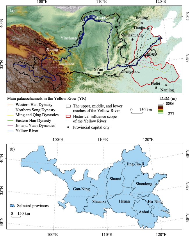
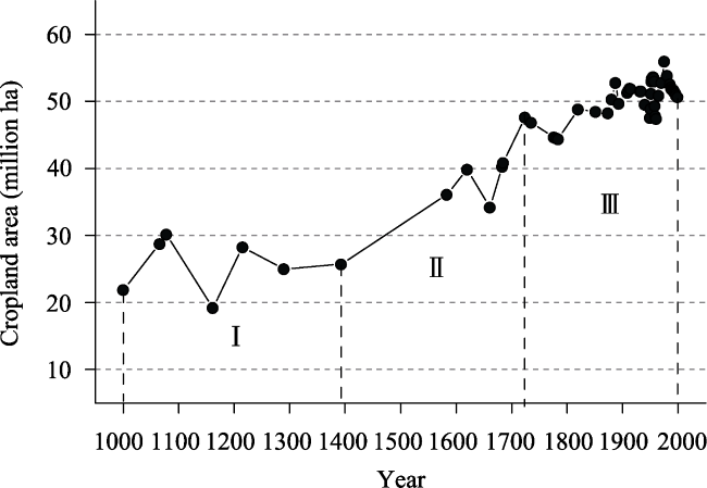
Landscape in the middle and lower reaches of the Yellow River in China has undergone significant changes for thousands of years due to agricultural expansion. Lack of reliable long-term and high-resolution historical cropland data has limited our ability in understanding and quantifying human impacts on regional climate change, carbon and water cycles. In this study, we used a data-driven modeling framework that combined multiple sources of data (historical provincial cropland area, historical coastlines, and satellite data-based maximum cropland extent) with a new gridding allocation model for croplands distribution to reconstruct a historical cropland dataset for the middle and lower reaches of the Yellow River at a 10-km resolution for 58 time points ranging from the period 1000 to 1999. The cropland area in the study area increased by 2.3 times from 21.87 million ha in 1000 to 50.64 million ha in 1999. Before 1393, the area of cropland increased slowly and was primarily concentrated in the Weihe and Fenhe plains. From 1393‒1820, the area of cropland increased rapidly, particularly on the North China Plain. Since 1820, cropland cover has tended to become saturated. Our newly reconstructed results agreed well with remotely sensed data as well as historical document-based facts regarding cropland distribution.
YANG Fan , ZHANG Hang , HE Fanneng , WANG Yafei , ZHOU Shengnan , DONG Guanpeng . A 1000-year history of cropland cover change along the middle and lower reaches of the Yellow River in China[J]. Journal of Geographical Sciences, 2024 , 34(5) : 921 -941 . DOI: 10.1007/s11442-024-2233-z
Figure 1 Study area (a. the Yellow River Basin and the scope of historical influence in the lower reaches of the Yellow River; b. provincial units) |
Table 1 Data sources for historical cropland cover in the middle and lower reaches of the Yellow River (DEM: digital elevation model; CPP: climate potential productivity) |
| Data variables | Temporal coverage | Spatial resolution | Data type | Data source/ Reference | |
|---|---|---|---|---|---|
| Historical cropland | Song, Liao, and Jin dynasties (1000, 1066, 1078, 1162, 1215) | Provincial level | Reconstructed values | Published literature | He et al. (2017); Li et al. (2018a) |
| Yuan Dynasty (1290) | Li et al. (2018b) | ||||
| Ming Dynasty (1393, 1583, 1620) | Li et al. (2020) | ||||
| Qing Dynasty to the present (1661-1999) (49 time points) | Ge et al. (2004); Li et al. (2016) | ||||
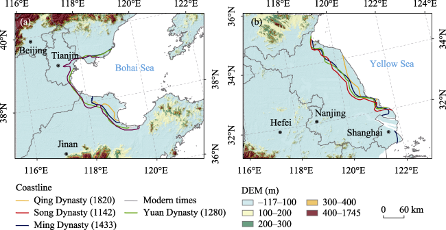
| Historical coastlines | Song Dynasty (1142) | Reconstructed vector lines | Historical Atlas of China | Tan (1982) | |
| Yuan Dynasty (1280) | |||||
| Ming Dynasty (1433) | |||||
| Qing Dynasty (1820) | |||||
| Remotely sensed land use data | 1980, 1990, 2000, 2010 | 1 km | Grid | Resources and Environmental Sciences Data Center of the Chinese Academy of Sciences, http://www.resdc.cn/ (last access: 10 February 2022) | |
| DEM | 2000 | 90 m | Grid | Resources and Environmental Sciences Data Center of the Chinese Academy of Sciences, http://www.resdc.cn/ (last access: 10 August 2022) | |
| CPP | 1951-1980 | 1 km | Grid | Data Sharing Infrastructure of Earth System Science, http://www.geodata.cn/ (last access: 10 August 2022) | |
Figure 2 Historical coastline over the past millennium (a. Coastlines in the western coast of Bohai Bay; b. northern coast of Jiangsu, and the Yangtze Estuary) |
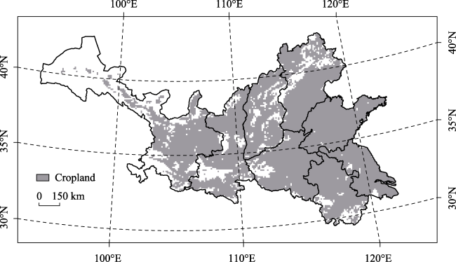
Figure 3 Remote sensing land use data-derived provincial maximum cropland allocation extent in the middle and lower reaches of the Yellow River |
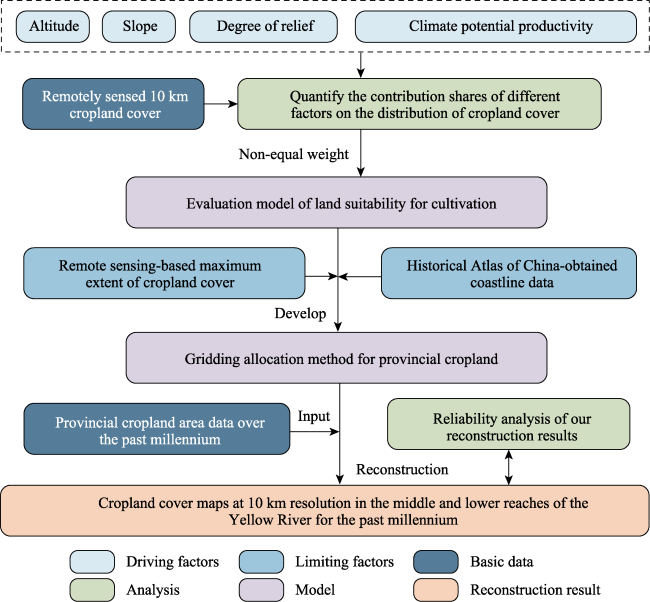
Figure 4 Scheme for gridding reconstruction of historical cropland cover in the middle and lower reaches of the Yellow River |
Table 2 Flow of Shapley value calculation. |
| Item | Definition | Formula |
|---|---|---|
| Step 1: Input profiles (T) | T, the universe of input profiles, represents the set of all possible input profiles. The universe with Nv factors will have 2Nv input profiles. | For example, for a three-factor model, the universe is: $\text{T}=\left\{ \left\{ 0,0,0 \right\};\left\{ 0,0,1 \right\};\left\{ 0,1,0 \right\};\left\{ 0,1,1 \right\} \right.;$ $\left. \left\{ 1,0,0 \right\};\left\{ 1,0,1 \right\};\left\{ 1,1,0 \right\};\left\{ 1,1,1 \right\} \right\}$ |
| Step 2: Shapley set (Q) | Q is defined the set of all input profiles in the universe of the model for which a certain factors is marked as a nonparticipant. | For example, in a three-factor model, the Shapley set for the third factor would be: $\begin{aligned}&\mathrm{m}\Big(\mathrm{v}\big(\vec{\mathrm{x}}\big),\mathrm{v}_{\mathrm{p}}\Big)=\mathrm{R}^{2}\Big(\mathrm{v}\big(\vec{\mathrm{x}}\big)+\mathrm{v}_{\mathrm{p}}\Big)-\mathrm{R}^{2}\Big(\mathrm{v}\big(\vec{\mathrm{x}}\big)\Big);\\&\mathrm{p\in1,2,...,N_{v}}\end{aligned}$ |
| Step 3: Marginal contribution (m) | When vp is added as a participant, the added value of R-squared is defined as the marginal contribution. | $\mathrm{m}\left(\mathrm{v}(\overrightarrow{\mathrm{x}}), \mathrm{v}_{\mathrm{p}}\right)=\mathrm{R}^{2}\left(\mathrm{v}(\overrightarrow{\mathrm{x}})+\mathrm{v}_{\mathrm{p}}\right)-\mathrm{R}^{2}(\mathrm{v}(\overrightarrow{\mathrm{x}})) ;$ $\text{p}\in 1,2,...,{{\text{N}}_{\text{v}}}$ $\mathrm{v}(\overrightarrow{\mathrm{x}})$denotes the variable set of the input profile. |
| Step 4: Shapley value (S) | $\mathrm{S\big(v_p\big)=\sum_{\vec{x}\in Q(T,p)}\frac{\big(\big|\vec{x}\big|\big)!\big(N_v-\big|\vec{x}\big|-1\big)!}{N_v !}m\big(v\big(\vec{x}\big),v_p\big)}$ | |
| Step 5: Relative important of factors (S%) | $S_{\%}\left(v_{p}\right)=\frac{S\left(v_{p}\right)}{\sum S(v)}$ | |
Table 3 Contribution shares of factors on the distribution of cropland cover |
| Jing-Jin-Ji | Shaanxi | Henan | Shanxi | Shandong | Anhui | Hu-Ning | Gan-Ning | |
|---|---|---|---|---|---|---|---|---|
| Altitude | 0.21 | 0.45 | 0.39 | 0.27 | 0.27 | 0.33 | 0.13 | 0.25 |
| CPP | 0.11 | 0.17 | 0.08 | 0.05 | 0.06 | 0.08 | 0.15 | 0.59 |
| DR | 0.41 | 0.24 | 0.33 | 0.42 | 0.39 | 0.30 | 0.51 | 0.11 |
| Slope | 0.27 | 0.14 | 0.20 | 0.26 | 0.28 | 0.30 | 0.20 | 0.05 |
CPP: Climatic potential productivity; DR: Degree of relief |
Table S1 Normalization formulas for altitude, CPP, DR, and slope |
| Factor | Relationship with cropland distribution | Formula |
|---|---|---|
| Altitude | Negative | ${{V}_{norm\_alti}}\left( i,j \right)=\frac{{{V}_{alti}}\left( i,max \right)-{{V}_{alti}}\left( i,j \right)}{{{V}_{alti}}\left( i,max \right)}$ |
| CPP | Positive | ${{V}_{norm\_CPP}}\left( i,j \right)=\frac{{{V}_{CPP}}\left( i,j \right)}{{{V}_{CPP}}\left( i,max \right)}$ |
| DR | Negative | ${{V}_{norm\_DR}}\left( i,j \right)=\frac{{{V}_{DR}}\left( i,max \right)-{{V}_{DR}}\left( i,j \right)}{{{V}_{DR}}\left( i,max \right)}$ |
| Slope | Negative | ${{V}_{norm\_slop}}\left( i,j \right)=\frac{{{V}_{slop}}\left( i,max \right)-{{V}_{slop}}\left( i,j \right)}{{{V}_{slop}}\left( i,max \right)}$ |
Note: positive characterizes that the larger the factor value, the more cropland distribution; negative characterizes that the larger the factor value, the less cropland distribution. Vnorm(i,j) represents the factor value of grid j in province i after the normalization; V(i,max) denotes the maximum factor value in province i; V(i,j) refers to the factor value of grid j in province i. |
Figure 5 Total cropland area in the middle and lower reaches of the Yellow River over the past millennium (Phase I: 1000-1393; Phase II: 1393-1724; Phase III: 1724-1999) |
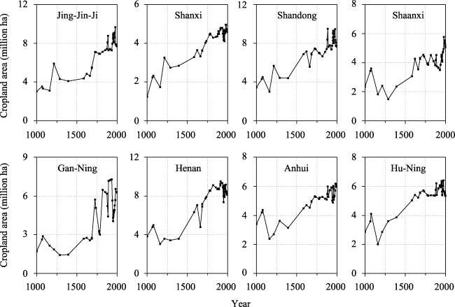
Figure 6 Provincial cropland area in the middle and lower reaches of the Yellow River over the past millennium |
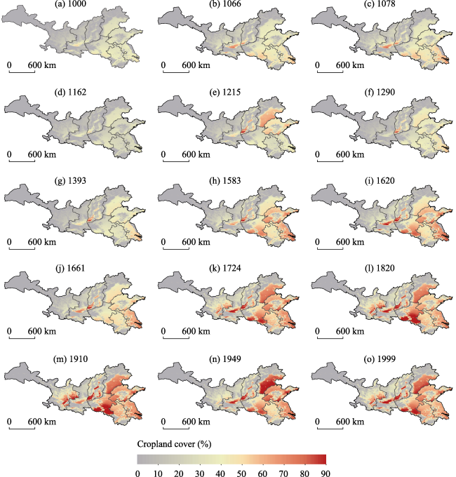
Figure 7 Cropland cover maps for the middle and lower reaches of the Yellow River over the past millennium (Panels a-o denote 1000, 1066, 1078, 1162, 1215, 1290, 1393, 1583, 1620, 1661, 1724, 1820, 1910, 1949, and 1999, respectively.) |
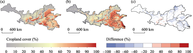
Figure 8 Spatial patterns of the allocation result (a), remote sensing-derived cropland cover in 1980 (b), and the differences between them (c) |
Table 4 Statistical value of differences in cropland cover in 1980 between allocation results and remote sensing-derived cropland cover |
| Difference (%) | Number of grids (%) | Difference (%) | Number of grids (%) |
|---|---|---|---|
| <-80 | 0.02 | 0-10 | 15.21 |
| -80 to -70 | 0.07 | 10-20 | 4.19 |
| -70 to -60 | 0.46 | 20-30 | 1.70 |
| -60 to -50 | 0.90 | 30-40 | 0.60 |
| -50 to -40 | 1.88 | 40-50 | 0.28 |
| -40 to -30 | 4.88 | 50-60 | 0.07 |
| -30 to -20 | 11.72 | 60-70 | 0.03 |
| -20 to -10 | 18.71 | 70-80 | 0.00 |
| -10 to 0 | 39.30 | >80 | 0.00 |
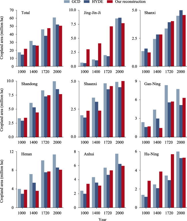
Figure 9 Comparison of total and provincial cropland area from the HYDE, GCD, and our reconstruction (HYDE: global environment database; GCD: global cropland dataset. Total denotes the entire middle and lower reaches of the Yellow River.) |
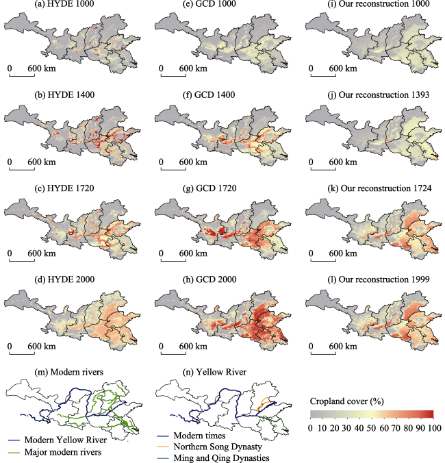
Figure 10 Comparison of cropland maps among three datasets (a-d. HYDE; e-h. GCD; and i-l. our reconstruction. Panels (m) and (n) represent modern rivers and Yellow Rivers in different periods. HYDE: global environment database; GCD: global cropland dataset.) |
| [1] |
|
| [2] |
|
| [3] |
|
| [4] |
|
| [5] |
|
| [6] |
|
| [7] |
|
| [8] |
|
| [9] |
|
| [10] |
|
| [11] |
|
| [12] |
|
| [13] |
|
| [14] |
|
| [15] |
|
| [16] |
|
| [17] |
|
| [18] |
|
| [19] |
|
| [20] |
|
| [21] |
|
| [22] |
|
| [23] |
|
| [24] |
|
| [25] |
|
| [26] |
|
| [27] |
|
| [28] |
|
| [29] |
|
| [30] |
|
| [31] |
|
| [32] |
|
| [33] |
|
| [34] |
|
| [35] |
|
| [36] |
|
| [37] |
|
| [38] |
|
| [39] |
|
| [40] |
|
| [41] |
|
| [42] |
|
| [43] |
|
| [44] |
|
| [45] |
|
| [46] |
|
| [47] |
|
| [48] |
|
| [49] |
|
| [50] |
|
| [51] |
|
| [52] |
|
| [53] |
|
| [54] |
|
| [55] |
|
/
| 〈 |
|
〉 |