Research Articles

Defining the land use area threshold and optimizing its structure to improve supply-demand balance state of ecosystem services

  • HUANG Pei , 1, 2 ,
  • ZHAO Xiaoqing , 1, 2, * ,
  • PU Junwei 1, 2 ,
  • GU Zexian 1, 2, 3 ,
  • RAN Yuju 1, 2 ,
  • XU Yifei 2 ,
  • WU Beihao 1, 2, 4 ,
  • DONG Wenwen 1, 2, 4 ,
  • QU Guoxun 4 ,
  • XIONG Bo 4 ,
  • ZHOU Longjin 4
Expand
  • 1. Institute of International Rivers & Eco-Security, Yunnan University, Kunming 650500, China
  • 2. School of Earth Sciences, Yunnan University, Kunming 650500, China
  • 3. Nujiang Forestry and Grassland Administration, Lushui 673100, Yunnan, China
  • 4. Yunnan Institute of Land Resources Planning and Design, Kunming 650200, China
*Zhao Xiaoqing (1969‒), Professor, specialized in land ecological security and territorial spatial optimisation. E-mail:

Huang Pei (1994‒), PhD Candidate, specialized in ecosystem service management and land use optimisation. E-mail:

Received date: 2023-08-23

  Accepted date: 2024-02-07

  Online published: 2024-05-31

Supported by

National Natural Science Foundation of China(42061052)

National Natural Science Foundation of China(41361020)

National Natural Science Foundation of China(40961031)

Joint Fund of Yunnan Provincial Science and Technology Department and Yunnan University(2018FY001-017)

Construction Project of Graduate Tutor Team in Yunnan Province(C176230200)

Postgraduate Innovative Research Project of Yunnan University(2020Z46)

Postgraduate Innovative Research Project of Yunnan University(2021T008)

Postgraduate Innovative Research Project of Yunnan University(KC-22222260)

Project of Joint Training Base for Postgraduate Integration Between Industry and Education in Yunnan Province(CZ22622203-2022-29)

Abstract

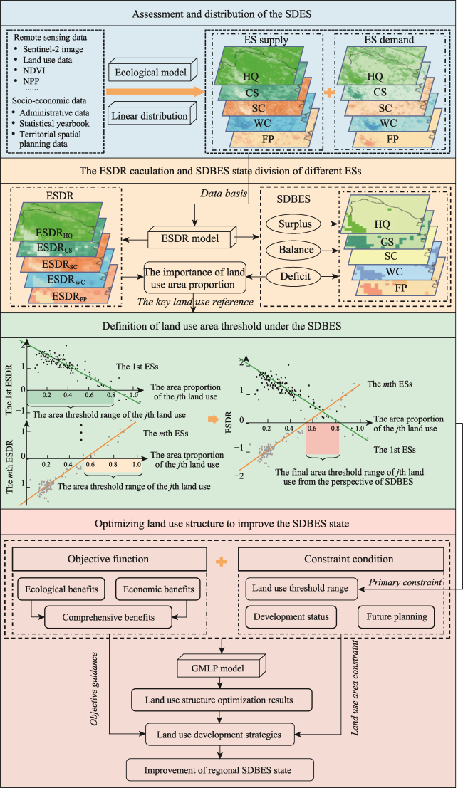
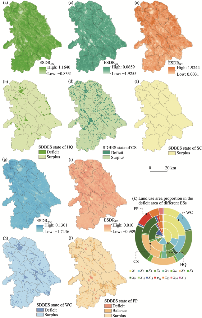
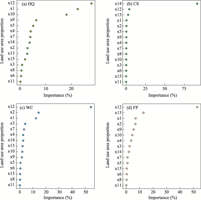
Improving the supply-demand balance of ecosystem services (SDBES) from the perspective of land use is essential for managing regional ecosystem and realizing sustainable development. By combining land use with the supply and demand of ecosystem services (SDES), a technical framework for defining land use threshold and optimizing its structure to improve the SDBES state was constructed and applied to a practical case. The spatial pattern of supply and demand of each ES in Lancang county was distinctly heterogeneous, with significant differences in SDES across different land use types. Strong spatial heterogeneity existed in the ESDR of each ES at the grid scale, and the areas of deficit were ranked as carbon sequestration > water conservation > habitat quality > food production. The structure of dry land, paddy field, tea, evergreen broad-leaved forest, grassland, urban construction land, and industrial and mining construction land were the focus of land use optimization. Based on the land use area thresholds under the SDBES, the optimal land use structure for maximizing comprehensive benefits contributed to a balanced relationship between SDES and promoted sustainable regional development. The study provides a new perspective and method for improving the SDBES state, alleviating land conflicts, and managing ecological environment.

Cite this article

HUANG Pei , ZHAO Xiaoqing , PU Junwei , GU Zexian , RAN Yuju , XU Yifei , WU Beihao , DONG Wenwen , QU Guoxun , XIONG Bo , ZHOU Longjin . Defining the land use area threshold and optimizing its structure to improve supply-demand balance state of ecosystem services[J]. Journal of Geographical Sciences, 2024 , 34(5) : 891 -920 . DOI: 10.1007/s11442-024-2232-0

1 Introduction

Ecosystem services (ESs) are the direct or indirect benefits that humans obtain from ecosystems (Mitchell et al., 2015; Niu et al., 2022). They play a key role in achieving sustainable development goals (SDGs) (Cochran et al., 2020; Reyers and Selig, 2020). The supply and demand of ecosystem services (SDES) are closely linked to natural ecosystems and socio- economic systems, which contribute to ecological security and sustainable socio-economic development (Qiu et al., 2022). With the rapid advancement of industrialization and urbanization, high-intensity human activities are increasingly interfering with ecosystems, causing a series of problems such as intense human-land conflicts, serious environmental pollution, and ecosystem degradation, which significantly affect the supply-demand balance of ecosystem services (SDBES) and threaten global and regional ecological security and sustainable development (Shao et al., 2018; Cochran et al., 2020; Delgado and Marín, 2020; Vargas et al., 2023). Therefore, how to improve the SDBES state is a topic worthy of further study.
SDES is the basis for the interaction between ESs and human well-being, and provides a decision for ESs management (Mehring et al., 2017; Chen et al., 2022; Zhang et al., 2022). Experts have increasingly recognised that regional ecological and environmental challenges mainly originate from the spatial differences and imbalances in SDES due to changes in urbanization and land use pattern (Cao et al., 2021; Lyu et al., 2022; Zhang et al., 2023). Therefore, supply-demand relationship has become a hot spot in the field of ESs. The research objects of SDES include provisioning, regulating, cultural, and supporting services (Castro et al., 2014; Czúcz et al., 2018). The research scales have expanded from small and medium levels such as streets, watersheds, basins, counties, provinces, and urban agglomerations (Larondelle and Lauf, 2016; Longato et al., 2023) to large national and global dimensions (Wolff et al., 2017; Grêt-Regamey and Weibel, 2020). The combination of multiple scales have gradually enriched the research in ESs (Bicking et al., 2018; Cui et al., 2019). However, the existing studies pay insufficient attention to mountainous counties with low levels of economic development and ecosystems that are greatly affected by human activities. The research methods of SDES include supply-demand relationship matrix, value evaluation, public participation and ecological model (Burkhard et al., 2012; Meraj et al., 2022). The ecological model based on the ecological process and mechanism is applied widely for its advantages in revealing the spatial heterogeneity of SDES (Grêt-Regamey and Weibel, 2020). The spatial distribution and balance pattern of SDES reflects the spatial allocation of resources and the benefits and limitations of ecosystem services to economic development (Chen et al., 2019). Understanding SDBES is conducive to promoting sustainable territorial spatial planning and improving the quality of life (Lorilla et al., 2019). In recent years, SDBES has become the frontier of ESs research (Jager et al., 2020; Sebastiani et al., 2021). Ecological supply-demand ratio (ESDR) is a key indicator for measuring the SDBES state of ESs (Zhao et al., 2022; Darvishi et al., 2023). The SDBES state can be classified as surplus, balance and deficit (Fu et al., 2021). Studies often use ESDR ≥ 0 as an important criterion to avoid regional supply-demand deficits (i.e., supply-demand imbalance) (Marino et al., 2021; Yuan et al., 2023). Studies have investigated the evolution, driving factors and development strategies of SDBES extensively (Yahdjian et al., 2015; Lorilla et al., 2019). However, no mature technical method to improve the SDBES state is currently available to fully support ecological and environmental management decisions. Balancing the SDES is still a major challenge.
Land is an important carrier of ecosystems, and is closely related to ESs via the interaction between human and environment (Hasan et al., 2020; Ma et al., 2023). The scarcity of land resources triggers land use competition and conflicts, resulting in changes in land use type, structure, pattern and function, which significantly change the structure and function of ESs (Olander et al., 2018; Xu et al., 2020; Peng et al., 2022). Therefore, land use is recognized as one of the most important factors that directly or indirectly influence regional SDES (González-García et al., 2020; Hasan et al., 2020). Although the impact of regional land use on ecosystems has received increasing attention, land types and landscape patterns are still being transformed and utilised in an unsustainable manner (Gomes et al., 2021). Besides, land use change directly affects the supply capacity of ESs, while human demand for ESs is also changing (Pătru-Stupariu et al., 2020). People usually want to maximize the supply of ESs via land use management to reduce mismatches and shortages (Chen et al., 2019; Xu et al., 2024). Previous studies investigating the relationship between ESs and land use have provided some ideas for improving the state of SDBES. The structural adjustment of land use is essential to ensure that the proportion of different land use types meets the threshold range for achieving the SDBES (Fu et al., 2021). Land use optimization is the most practical approach to adjust land use structure, which provides support for the sustainability of land resources (Albert et al., 2015; Jiang et al., 2021a; Shao et al., 2023). The optimization of land use structure under the SDBES is conducive to enhancing the policy relevance of the ecosystem in land management and planning and effectively reducing the spatial mismatch of ESs, which is of great significance for strengthening ESs management and achieving ecological security (Wu et al., 2018). Some studies have proposed a framework for balancing the SDES, which is related to land use. Based on regression analysis of ESDR and construction land and green space, the land use area threshold was used to improve the relationship between SDES (Chen et al., 2019). However, the aforementioned studies do not meet the requirements for improving the state of SDBES in regions with complex land use types. In addition, exploring a win-win strategy to balance ecosystem protection and socio-economic development is key to sustainable land use (Mazziotta et al., 2016; Rahman and Szabó, 2021). How to adjust the land use structure and determine its optimal threshold to improve the state of SDBES is still a major challenge. To the best of our knowledge, the current studies improving the state of SDBES rarely involve land use optimization, and do not address regional comprehensive developmental objectives. Thus, it is difficult to promote a coordinated ecological environmental protection and socio-economic development. It has limited significance in guiding regional territorial spatial planning as well as ecological and environmental management. In this context, defining the land use threshold and optimizing its structure under the SDBES are essential for the integration of land use into strategies for improving the state of SDBES.
Southwest Yunnan province is a region in China with complex geographical environment, rich biodiversity, fragile ecological environment and relatively backward economic development (Huang et al., 2023). Lancang is an ethnic county in the plateau and mountains of southwest Yunnan. It is an important node for the territorial spatial planning of Yunnan. It is also an agricultural area and an ecological barrier with a prominent role in economic development and ecological protection of Yunnan. Therefore, despite the tremendous opportunities for development, Lancang also faces the challenge of coordinating the relationship between ecological environmental protection and economic development. Further, the rapid urban expansion and construction, the large-scale introduction of economic forests, and the development of infrastructure such as airports and hydropower stations have intensified the contradictions and conflicts between humans and land use in the county. These factors significantly affect the structure and land use pattern and thereby transform the structure and function of the original ecosystem (Zhao and Xu, 2015; Zhao et al., 2021). This inevitably affects the structure and balance of SDES in the county. However, what are the characteristics of the current global and local patterns of SDBES in the study area? How to combine the SDES and the comprehensive objective of land use development to optimize the land use structure to better improve the state of SDBES and promote a coordinated ecological protection and economic development? These are the key scientific questions that need to be solved through research. Accordingly, this study constructed a novel technical framework for defining land use area thresholds and conducting multi-objective optimization under the SDBES to improve its regional state. Then, Lancang county was taken as the study area to measure and analyse the supply-demand balance patterns of five typical ESs. Based on the area threshold of land use under the SDBES, the comprehensive objective including ecological and economic benefits was combined to optimize land use structure in 2035, and land use development strategies were proposed to support the SDBES. It aims to provide methodological and technical support for improving the state of SDBES from the perspective of land use, as well as to support the ecological and environmental management and the sustainable development in the study area and other similar areas.

2 Materials and methodologies

2.1 Technical framework

The technical framework is presented in Figure 1. First, based on the natural factors and socio-economic data in 2020, the supply and demand of all kinds of ESs in Lancang county were calculated. Second, based on the ESDR, the SDBES state of each ES was classified. The key land use types contributing to the deficit of SDES were identified, which provided objects reference for the land use structural adjustment in the future. Third, the land use area thresholds under the SDBES, obtained by the regression analysis of ESDR and land use area proportion, were defined as the primary constraint for the optimization of land use structure in 2035. Finally, after considering the land use thresholds, the current land use development status and the future demands for land use and combining with comprehensive objective, the grey multi-objective linear programming (GMLP) model was used to optimize land use structure, and corresponding land use development strategies for the future were proposed to better support regional SDBES.
Figure 1 Technical framework

2.2 Study area and data sources

2.2.1 Study area

Lancang county (99°29′-100°35′E, 22°01′-23°16′N), a border county in southwest China, belongs to Puer city, Yunnan province (Figure 2). It is located in the south of the Hengduan Mountains with an area of 8807 km2, and the mountainous area accounts for 98.8%. The climate in Lancang is mainly subtropical monsoon type, with an average annual temperature of 19.1℃ and an annual rainfall of 1626.5 mm. The rivers in Lancang county belong to the Lancang River system, and the soil type is predominantly lateritic red earth. Forest and cropland were the dominant land use types in 2020 (Figure 1). Subtropical evergreen broad-leaved and coniferous forests represent the zonal vegetation. Simao pine, eucalyptus, rubber and tea are the main economic forests (Huang et al., 2023). By the end of 2020, the population of 441,500 with an urbanization rate of 37% in Lancang county contributed to a GDP of 12.07 billion yuan. It is an important agricultural county in China. It is also located in the tropical forest ecological barrier area and urban development zone on the southern border of Yunnan, with a prominent ecological status and a significant socio-economic role. Large-scale human activities have changed the land use structure and the ESs of the county (Gu et al., 2016; Zhao et al., 2021). Improving the SDBES state, promoting coordinated ecological protection and socio-economic development, and forming a green and sustainable land use development pattern are the scientific challenges faced by Lancang county.
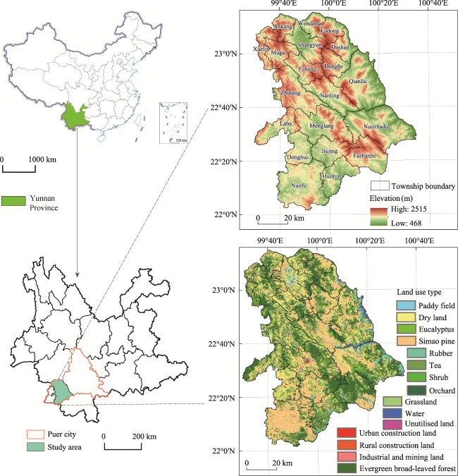
Figure 2 The geographic location and land use types (2020) of Lancang county, Yunnan province, southwest China

2.2.2 Data sources

The datasets include natural data and socio-economic data (Table 1). The land use data in 2020 was derived from the remote sensing interpretation results extracted by the random forest model with auxiliary factors (RF-AFs) model (Huang et al., 2023). Referring to the land use/cover classification system of the Chinese Academy of Sciences and considering the actual situation in the study area, the lands were further classified into cropland (dry land, paddy field), plantation (orchard, tea, rubber), forests (eucalyptus, Simao pine, shrub, and evergreen broad-leaved forest), grassland, water, construction land (urban construction land, rural construction land, industrial and mining construction land) and unutilised land. A total of 7 first-level and 15 second-level land use types were classified (Figure 2). The second-level land use types represent decision variables in the land use structure optimization model, which were denoted by x1, x2, x3, x4, x5, x6, x7, x8, x9, x10, x11, x12, x13, x14, and x15, respectively. All spatial data were unified to a resolution of 30 m × 30 m.
Table 1 Data names and sources
Date type Data name Resolution Data source
Natural data Sentinel-2 image 10 m × 10 m United States Geological Survey (https://earthexplorer.usgs.gov/)
NDVI 10 m × 10 m Calculated from the band of satellite images
DEM 30 m × 30 m Geospatial Data Cloud (https://www.gscloud.cn/sources)
Soil type / China soil map based harmonized world soil database (https://data.tpdc.ac.cn/zh-hans/)
Tempreture 30 m × 30 m National Earth System Science Data Center,
National Science & Technology Infrastructure
of China (http://www.geodata.cn)
Precipitation 30 m× 30 m National Earth System Science Data Center,
National Science & Technology Infrastructure
of China (http://www.geodata.cn)
NPP 500 m × 500 m LAADS DAAC (https://ladsweb.modaps.eosdis.nasa.gov/)
Evapotranspiration 500 m × 500 m LAADS DAAC (https://ladsweb.modaps.eosdis.nasa.gov/)
Socio-economic data Administrative boundary / The People’s Government of Lancang County (http://lancang.gov.cn/)
Statistical Yearbook of Lancang County / Statistics Bureau of Lancang County
Statistical Yearbook of Yunnan Province / Statistics Bureau of Yunnan Province (http://stats.yn.gov.cn/)
Population density 100 m × 100m WorldPop (https://www.geodata.cn/)
Territorial Spatial Planning of Lancang County (2021-2035) / The People’s Government of Lancang County (http://lancang.gov.cn/)

2.3 Methods

2.3.1 Measurement of supply and demand of ecosystem services (SDES)

Based on the relative importance of different ecosystems for human well-being, the representativeness of major ecosystem categories, and data availability, five key ESs including habitat quality (HQ), carbon sequestration (CS), soil conservation (SC), water conservation (WC), and food production (FP) were selected to calculate their SDES. We have made local parametric corrections in the SDES calculation process to compensate for errors caused by the uniform resolution of some original indicators. The specific calculation and correction methods are detailed in the Appendix.
(1) Supply and demand of habitat quality (HQ)
The HQ supply was calculated using the InVEST model (Terrado et al., 2016). The average value of HQ supply in the study area represented the demand standard. The HQ demand of each pixel was defined as the difference between the demand standard and the HQ supply (Shi et al., 2020).
(2) Supply and demand of carbon sequestration (CS)
Plant biomass reflects the CO2 sequestered by terrestrial ecosystems (Lal et al., 2018). CS supply was calculated based on the photosynthesis and respiration of vegetation (Han and Ouyang, 2021). CS demand is characterised by regional carbon emissions. Referring to the CO2 emissions of Puer city in agriculture, service, industry, and construction sectors established in 2020, according to the socio-economic structure characteristics of Puer city and Lancang county, the total carbon emissions of each sector in Puer city were attributed to each land use type in Lancang county (Table 2).
Table 2 CO2 emission allocation in Lancang county
Classification CO2 emission in Puer (megaton) Basis of distribution CO2 emission in Lancang (megaton) Land use of allocation
Agriculture 74 Primary production 9.61 Cropland (dry land and paddy field)
Service industry 18 Resident population 3.30 Urban construction land
Industry 487.62 Industrial output value 85.60 Industrial and mining construction land
Building industry 323 Construction output value 36.03 Urban construction land
Urban life 3 Urban population 0.32 Urban construction land
Rural life 17 Rural population 4.02 Rural construction land
Road 125 Total road mileage 44.44 Urban and rural road
Aviation 7 Resident population 1.29 Whole study area
Total 1055 / 184.61
(3) Supply and demand of soil conservation (SC)
The revised universal soil loss equation (RUSLE) was used to estimate the amount of soil conservation and soil erosion (Kwanele et al., 2019). The amount of the soil conservation and soil erosion represented SC supply and SC demand, respectively (Fu et al., 2021).
(4) Supply and demand of water conservation (WC)
The WC supply was measured by correcting the water yield that calculated using the InVEST model based on soil depth, soil saturated hydraulic conductivity, topographic index and velocity coefficient (Cui et al., 2019; Sharafatmandrad and Khosravi Mashizi, 2021). WC demand is the total amount of water used for agriculture, ecology, life and industry (González-García et al., 2020). Agricultural water was allocated to cropland according to normalized difference vegetation index (NDVI). Ecological water was allocated to forest and grassland according to NDVI. Domestic water was allocated to urban construction land and rural construction land according to population density. Industrial water was allocated to industrial and mining construction land according to population density.
(5) Supply and demand of food production (FP)
Based on the main agricultural and fishery production in Lancang county, the FP supply was converted to actual energy by referring to the China Food Composition Table (Yang et al., 2018). The total energy of different foods was evenly allocated to each land use type according to NDVI (Liu et al., 2022). The energy of grain crops, oil plants, sugar crops and vegetables were allocated to dry land and paddy field. The fruit energy was allocated to orchard, whereas meat, poultry and eggs energies were attributed to dry land, paddy field and grassland. The aquatic products energy was allocated to water. According to the China Food and Nutrition Development Program (2014-2020), the daily energy intake per capita in China is 2200-2300 kcal. In this study, 2300 kcal was taken as the standard, and the per capita annual energy intake standard was 839500 kcal. FP demand was calculated based on the per capita annual energy intake and the revised population density (Chen et al., 2020a).

2.3.2 Ecological supply-demand ratio (ESDR) calculation and supply-demand balance of ecosystem services (SDBES) state zoning

ESDR is used to reflect the SDBES state of ESs (i.e., surplus, balance, and deficit levels). The methods of ESDR calculation and SDBES state zoning are as follows:
$\left\{ \begin{align} & ESD{{R}_{im}}=\frac{ES{{S}_{im}}-ES{{D}_{im}}}{(ES{{S}_{m}}\max +ES{{D}_{m}}\max )/2} \\ & ESD{{R}_{im}}\text{}0,Surplus \\ & ESD{{R}_{im}}=0,\text{Balance} \\ & ESD{{R}_{im}}\text{}0,\text{D}eficit \\ \end{align} \right.$
where ESDRim is the ESDR of the mth ES in the ith gride; ESSim denotes the supply of the mth ES in the ith gride; ESDim represents the demand of the mth ES in the ith gride; ESSmmax refers to the max supply of the mth ES; and ESDmmax is the max demand of the mth ES. If ESDRim < 0, ES is deficit; if ESDRim = 0, ES is absolute balanced; and if ESDRim > 0, ES is surplus. In this study, the SDBES goal is achieving ESDRim≥0 through land use adjustment and optimization, rather than absolute balance (ESDRim=0).

2.3.3 Optimal granularity selection

The landscape pattern of land use has significant scale dependence on the ESs (Fu et al., 2011; Bai et al., 2020). To further explore the relationship between the proportion of each land use type and the ESDR, it is particularly important to unify and determine the optimal granularity (i.e., the grid size). Landscape connectivity is an important index, which can be used to determine the optimal granularity of land use. Based on the land use of Lancang county in 2020, connectance index (CONNECT), number of patches (NP) and patch density (PD), which represent the landscape connectivity (Zhang et al., 2020; Penagos Gaviria et al., 2022), were used to determine the optimal granularity. As shown in Figure 3, when the granularity is 1000, the CONNECT of the study area reached the maximum value and the decrease in NP and PD was stabilised. Therefore, 1000 m × 1000 m was regarded as the optimal granularity.
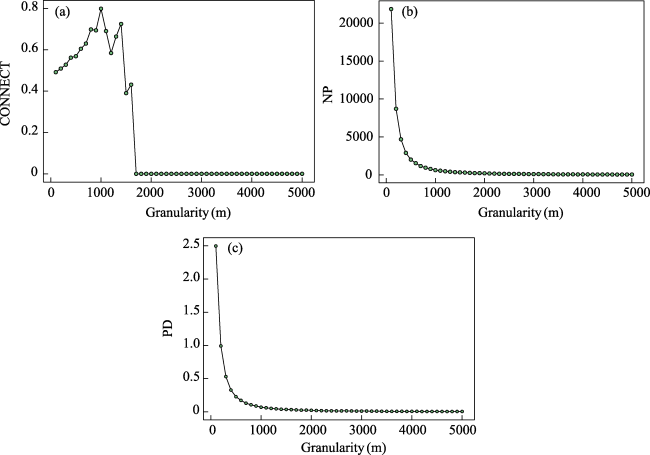
Figure 3 Landscape pattern index changes at different granularity levels (a. CONNECT; b. NP; c. PD)

2.3.4 Ordinary least squares regression mode

The ordinary least squares regression (Mirchooli et al., 2023) was applied to explore the relationship between the ESDR and the area proportion of land use types. This study selected simple linear, polynomial, and multiple linear regression models. Using the RStudio platform, the trend lines between the area proportion of each land use type and the ESDR of each ES were plotted, and their optimal regression models were chosen based on fitting degree (R2) and significance (p-value). Regression curves with relatively high R2 and low p-values (< 0.001) were retained. Then, based on the results of regression analysis, the area threshold range of each land use type under the SDBES was comprehensively defined.

2.3.5 Grey multi-objective linear programming (GMLP) model

The GMLP model combines the grey model and multi-objective linear programming approaches to determine the optimal land use optimization solution for decision makers (Darvishi et al., 2020). Based on the land use threshold under the SDBES, the GMLP model was used to solve the optimal land use structure to achieve the maximum comprehensive benefits in Lancang in 2035 to improve the SDBES state. The principles of the GMLP model are as follows:
$\left\{ \begin{align} & f(x)=\sum\limits_{j=1}^{m}{{{c}_{j}}\times {{x}_{j}}\to \max (\min )} \\ & \sum\limits_{j=1}^{m}{{{a}_{ij}}\ge (\le ){{b}_{i}}} \\ & {{x}_{j}}\ge 0\text{ }(j=1,2,3...,n) \\ \end{align} \right.$
where f(x) is the objective function; cj is the benefit coefficient; xj denotes the decision variable; aij represents the constraints; bi refers to the constraint constants, which were obtained by the predicted results of the GM(1,1) model or relevant policy planning of Lancang county.
In this study, the comprehensive benefits included ecological and economic benefits. The objective of maximizing comprehensive benefits contributed to optimal ecological and economic benefits simultaneously. The ecological benefit function was constructed using the ecosystem service value (ESV). The equivalent factor method was used to calculate the ESV per unit area of various types of non-construction land (Costanza et al., 1997; Xie et al., 2017). The ESV per unit area of construction land was calculated based on relevant research (Xie et al., 2021; Ran et al., 2022). The economic benefit function was constructed based on the economic benefits per unit area and the area of various land use types (Zhang et al., 2016). The economic value of crops such as grain, vegetables, and sugar cane was allocated to dry land and paddy field. The economic value of fruits was attributed to orchard. The economic value of fisheries was associated with water. The economic value of rubber was linked to rubber. The economic value of tea was assigned to tea. The economic value of animal husbandry was attributed to grassland; the economic value of forestry (except for rubber) was allocated to eucalyptus and Simao pine. The value of agricultural services was related to rural construction land, and the economic value of the secondary and tertiary industries was traced to urban construction land and industrial and mining land. Accordingly, the economic benefit of the area per unit of each land use type was calculated. The comprehensive benefits can be represented by the following equation:
$MaxCB=\sum\limits_{j=1}^{J}{(ES{{V}_{j}}}+E{{B}_{j}})\times {{S}_{j}}$
where$M\text{ax}CB$is the function denoting maximum comprehensive benefits; ESVj is the ESV per unit area of the jth land use type; EBj represents the economic benefit coefficient per unit area of the jth land use type; Sj indicates the area of the jth land use type; and J is the total number of land use types (J = 15).

3 Results

3.1 Spatial pattern of different SDES

The spatial pattern of supply and demand of each ES is shown in Figure 4, and the mean ES supply and mean ES demand values of different land use types are presented in Table 3. The mean HQ supply in the study area was 0.7649. The areas with high HQ supply were mainly located in the rubber, eucalyptus, Simao pine, shrub, evergreen broad-leaved forest and grassland in the southern and central segments of the study area, which also indicates that economic forests such as eucalyptus, Simao pine and rubber contribute significantly to regional HQ supply. However, the overall HQ demand was relatively low, with an average value of 0.1538. The spatial distribution of areas with high HQ demand and high HQ supply complemented each other. The high HQ demand was concentrated in the central and northern construction land and cropland. These areas experience high intensity of human interference, posing a stronger threat to biodiversity and biological habitat quality.
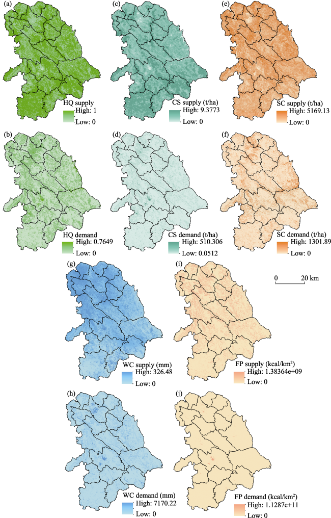
Figure 4 Spatial pattern of supply and demand in different ecosystem services (ESs) in Lancang county
Table 3 Mean ecosystem services supply and demand values of different land use types in Lancing county
Land use type HQ supply HQ
demand
CS supply (t/ha) CS demand
(t/ha)
SC
supply (t/ha)
SC demand
(t/ha)
WC
supply (mm)
WC
demand (mm)
FP
supply (kcal/km2)
FP
demand (kcal/km2)
x1 0.2975 0.4673 3.8058 0.3548 692.7669 15.6646 82.3738 39.0691 6.9384×10⁸ 0.0000
x2 0.3052 0.4597 3.5275 0.3548 478.1166 0.7387 85.0346 449.3223 5.3524×10⁸ 0.0000
x3 0.5685 0.2726 4.5113 0.0512 646.1845 16.5111 109.0222 1202.4535 4.1463×10⁸ 0.0000
x4 0.3802 0.3847 4.1202 0.0512 665.5980 6.5620 267.1822 0.3091 0.0000 0.0000
x5 0.9062 0.0000 5.7855 0.0512 798.8708 10.7828 40.6318 0.3217 0.0000 0.0000
x6 0.9979 0.0000 7.2750 0.0512 800.8780 1.0878 55.6357 0.4651 0.0000 0.0000
x7 0.9981 0.0000 6.7848 0.0512 784.7157 4.0071 48.3214 0.4130 0.0000 0.0000
x8 0.9960 0.0000 4.1470 0.0512 965.9204 7.3143 226.5733 0.3964 0.0000 0.0000
x9 0.9962 0.0001 6.9233 0.0512 834.9555 3.1431 60.6951 0.4378 32286.1228 0.0000
x10 0.7611 0.0038 3.4880 0.0512 737.9164 22.1801 102.4624 0.3118 1.1172×10¹⁰ 0.0000
x11 0.1630 0.6019 0.0000 0.0512 559.6692 0.0578 0.6950 0.0000 1.3421×10⁸ 0.0000
x12 0.0000 0.7649 0.0000 97.9466 276.7624 0.0296 279.3969 1032.3706 0.0000 23405.8948
x13 0.0014 0.7636 0.0099 38.9083 589.6860 0.0950 274.3689 29.0935 0.0000 535.0919
x14 0.2990 0.4962 2.4503 510.3055 406.1907 18.8847 160.5418 265.7756 0.0000 2118.1815
x15 0.0332 0.7317 0.0000 0.0512 614.9947 57.9809 264.5853 0.0000 0.0000 0.0000
The mean CS supply is 5.7052 t/ha. The overall CS supply showed a high value in the south and low value in the north, with the high CS supply areas concentrated in the south in the areas of eucalyptus, Simao pine, rubber, and evergreen broad-leaved forest. It indicates that evergreen broad-leaved forest and economic forest play an important role in enhancing CS. The mean CS demand was 2.0962. The areas with high CS demand were concentrated in the central and northern construction land. The mean CS demand of industrial and mining construction land was the highest, reaching 97.9466 t/ha. Industrial development requires the burning of a large amount of fossil fuels, resulting in the highest actual emissions of CO2 from industrial and mining construction land.
The mean SC supply in the study area was 763.360 t/ha. The high SC supply areas were mainly located in the forest and grassland areas in the central, eastern, and northwest regions. Among them, the SC supply of forest was generally higher. Lancang is located in the subtropical monsoon climate zone, with suitable temperatures and abundant precipitation, which are conducive to plant growth and the development of plant roots. This contributes to the stronger soil conservation capacity in forest areas. The mean SC demand was 6.1835 t/ha. The high SC demand areas were mainly located in dry land, orchard, industrial and mining construction land, grassland, and unutilised land in the east, west and north regions. The above regions exhibit abundant precipitation, large undulating terrain, steep slopes, and strong interference from human activities, so soil erosion is more prominent than other places.
The spatial pattern of WC supply was high in the north and low in the south, and the mean WC supply was 82.2289 mm. The high WC supply was mainly observed in the northern evergreen broad-leaved forest, shrub, orchard, tea, dry land and paddy field areas due to higher precipitation in the south and lower precipitation in the north of Lancang. Despite strong evapotranspiration, the higher WC supply is attributed to high precipitation, dense vegetation, and strong water retention capacity in these areas. Further, there was a high WC supply area in the southeast of the study area due to the lower evapotranspiration intensity and higher soil water retention capacity. The mean WC demand was 29.6706 mm, and the high WC demand areas are mainly located in the central urban construction land and industrial and mining construction land, as well as the northern urban construction land and paddy field areas. Menglang is the administrative center of the county in the central portion of the study area, with a high level of economic development, high population density, a large consumption of urban domestic water and industrial and mining production water, leading to relatively higher WC demand. In the northern areas with high WC demand, in addition to urban distribution, a widespread distribution of paddy fields and orchards was observed. The high demand for water for both domestic and agricultural irrigation purposes contributed to the high WC demand.
The mean FP supply in the study area was 1.5862 × 10⁸ kcal/km2. The overall FP supply showed a high spatial pattern in the north and a low spatial pattern in the south. The high FP supply distribution pattern was consistent with dry land, paddy field, orchard, grassland and water. The mean FP supply of grassland was significantly higher than that of other land use types. Animal husbandry based on grasslands provides abundant food products and energy sources. The mean FS demand was 0.4430 × 10⁸ kcal/km2, and the high distribution pattern of FS demand area was consistent with that of construction land. FS demand is directly related to population distribution, with Menglang in the central part of the study area having the highest population density, resulting in the highest FS demand.

3.2 ESDR and SDBES state of different ESs

The land use data and the SDES data at the pixel scale (30 × 30 m) were unified to the grid cell (1 × 1 km). Based on equation 2, the ESDR of each ES was calculated for different grid cells, and their SDBES regions were classified (Figure 5). Overall, the mean ESDRHQ, ESDRCS, ESDRSC, ESDRWC, and ESDRFP in Lancang county were 0.6793, 0.0247, 0.8658, 0.0235, and 0.0017, respectively, which were all greater than 0, indicating that the mean supply of each ES was greater than the mean demand, that is, each ES represents a supply-demand surplus at the county scale. However, ESDR and SDBES are scale-dependent, and the imbalance between SDES was more prominent at the grid scale (Figure 5).
Figure 5 The ecological supply-demand ratio (ESDR), supply-demand balance of ecosystem services (SDBES) state, and land use proportion (in the deficit area) of different ecosystem services (ESs) in Lancing county
The spatial patterns of ESDRHQ and ESDRCS showed a relatively consistent characteristic. The areas with high ESDRHQ and ESDRCS were mainly concentrated in the eucalyptus, Simao pine, shrub, and evergreen broad-leaved forest in the central and southern towns. The areas with low ESDRHQ and ESDRCS were mainly concentrated in the dry land and paddy field in the central and northern towns, as well as in the central construction land. The areas with high ESDRSC were consistent with high SC supply, and were mainly distributed in the forest and grassland in the central, eastern, and northwestern towns. These areas have dense vegetation, are located at a higher altitude, and have less human disturbance and stronger soil conservation capacity. The areas with high ESDRWC were mainly distributed in evergreen broad-leaved forest, shrub, eucalyptus, Simao pine, and grassland in the southern and northwestern towns. These areas have strong soil water retention capacity, so the WC supply is greater than the WC demand. The areas with low ESDRWC were mainly distributed in dry land, paddy field, urban construction land, and rural construction land. The high demand for agricultural production water and domestic water consumption in these areas resulted in relatively low ESDRWC, and even negative values. ESDRFP showed a high spatial distribution in the north and low distribution in the south. The high ESDRFP areas were mainly distributed in dry land, paddy field, and grassland. The aforementioned areas represent the main areas associated with grain production and animal husbandry development in the study area. They are the main areas associated with high food supply capacity with the development of agricultural technology. The areas with low ESDRFP were consistent with the spatial pattern of construction land. These areas have a relatively concentrated population, smaller food supply, and higher food demand.
The division results of the SDBES state area for each ES suggested that the remaining four ESs except SC include deficit and surplus areas, and the surplus areas were greater than that of deficit areas. The spatial pattern of deficit areas of each ES was relatively consistent with their low ESDR areas, and the area of deficit showed the characteristic of CS (12.09%) > WC (8.30%) > HQ (3.66%) > FP (1.78%). The land use structure within the deficit areas of ESs was shown in Figure 5k. The circular diagram showed each land use area proportion within the deficit zones of HQ, CS, WC, and FP from inside to outside. However, the area of different land use types in the ESs deficit area had different effects on the degree of ESs deficit. The random forest model was used to calculate the relative importance of each land use area. As shown in Figure 6, the cumulative importance of land use area such as dry land, tea, evergreen broad-leaved forest, grassland, urban construction land to ESDRHQ was about 83.97%, indicating that these land use types have a greater impact on the deficit of HQ. As for CS, the cumulative importance of the land use area such as urban construction land and industrial and mining construction land reached 95.42%, indicating that the two lands were important carbon sources, which affect the deficit of CS. As for WC, the cumulative importance of the paddy field, urban construction land, and industrial and mining construction land reached 81.07%, indicating that the large-scale water consumption in agriculture, industrial production, and urban life was the primary factor contributing to the deficit of WC. As for FP, the cumulative importance of dry land, paddy field, evergreen broad-leaved forest, urban and rural construction land reached 84.89%, indicating that these land use types strongly affected the deficit of FP. Overall, the structures of dry land, paddy field, tea, evergreen broad-leaved forest, grassland, urban construction land, rural construction land, and industrial and mining construction land need to be paid more attention in the future.
Figure 6 Importance of each land use area proportion to ecological supply-demand ratio (ESDR) in different ecosystem services (ESs) deficit areas

3.3 Land use threshold under the SDBES

The regression results of the ESDR of various ESs and the areas proportion of various land use types were shown in Figure 7. Generally, the ESDR of the remaining ESs showed a trade-off with other land use types excluding the synergistic relationship between ESDRHQ and cropland area proportion, based on the retained regression curves.
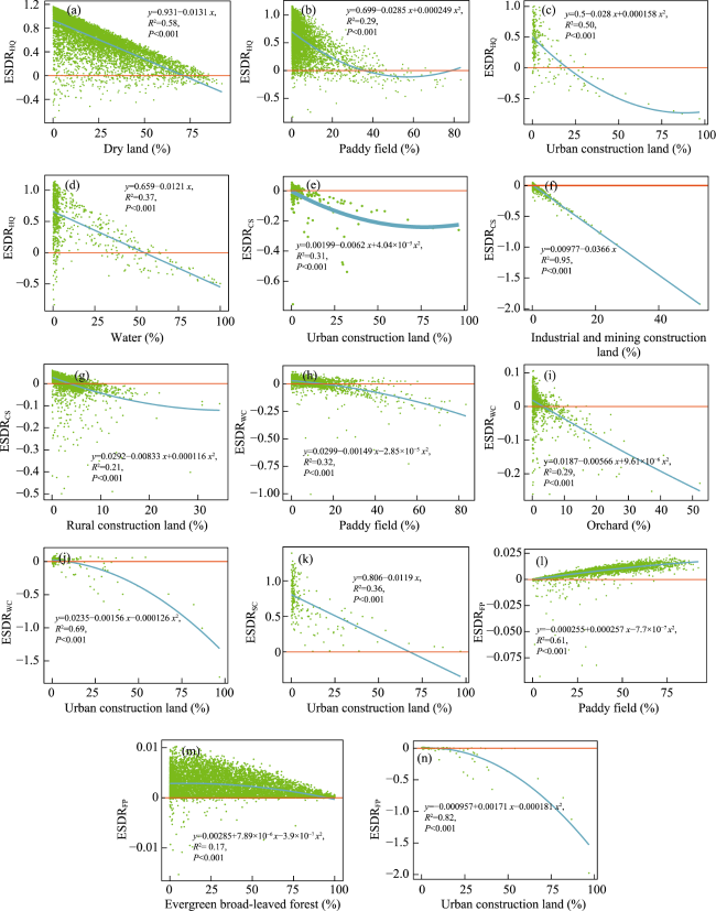
Figure 7 Regression relationship between ecological supply-demand ratio (ESDR) and land use area proportion
In terms of ESDRHQ, dry land, paddy field, and urban construction land showed significant stress due to specific human activities on the habitats. The higher their area, the greater the impact of human activities on the structure and function of HQ. Besides, high HQ demand in these land use types led to a decrease in ESDRHQ as their area increased. The threshold ranges for the proportion of above three land use types to achieve a supply-demand balance of HQ were (0, 71.07%], (0, 35.60%], and (0, 20.15%], respectively. The trade-off between water proportion and ESDRHQ is attributed to the large demand for water in urban construction, rural construction as well as industrial and mining construction activities, resulting in obvious effects on adjacent rivers and reservoirs. The threshold range for the proportion of water to achieve a supply-demand balance of HQ was (0, 54.46%].
In terms of ESDRCS, a significant trade-off existed between the areas of construction land and ESDRCS, and the R2 of the regression curve between the proportion of industrial and mining construction land and ESDRCS was the highest (up to 0.95). Three kinds of construction lands involve large-scale human activities and are important carbon sources. Their carbon emission intensity is large, and the CS demand is very high. Therefore, ESDRCS decreased as the area of these land use types increased. The threshold ranges for the proportion of the three land use types mentioned above to achieve a supply-demand balance of CS were (0, 0.32%], (0, 0.27%], and (0, 3.69%], respectively.
In terms of ESDRWC, the trade-off existed between the land use types such as paddy field, orchard, and urban construction land and ESDRWC was more significant. These lands consume large amounts of water. They are mostly distributed in areas with abundant water such as rivers and reservoirs. Crop growth and urban development require a substantial amount of water. Further, due to limited WC capacity of the three land use types, the ESDRWC decreased as their areas increased. The threshold ranges for the proportion of the three lands to achieve a supply-demand balance of WR were (0, 15.48%], (0, 3.32%], and (0, 8.80%], respectively.
In terms of ESDRSC, although the values were greater than 0, a significant trade-off existed between ESDRSC and the proportion of urban construction land. ESDRSC is mainly affected by vegetation cover and soil conservation measures. As the area of urban construction land increases, the vegetation coverage decreases and the soil conservation measurement factor tends to be 0, leading to a decrease in ESDRSC. The threshold range for the proportion of the urban construction land to achieve a supply-demand balance of SC was (0, 67.73%].
In terms of ESDRFP, a significant synergistic relationship was found between the proportion of dry land and ESDRFP, while a trade-off existed between the land use types such as construction land and evergreen broad-leaved forest and ESDRFP. Dry land is the main cropland in the study area, constituting 19.91%. The higher the area of dry land, the higher the grain yield per unit area. Besides, with the implementation of the Grain for Green Project and the occupation of agricultural land due to urban construction, the higher the area of evergreen broad-leaved forest and urban construction land, the lower the FP supply. The threshold ranges for the proportions of dry land, urban construction land, and evergreen broad-leaved forest to achieve supply-demand balance of FP were (0.99%, 100%], (0, 95.25%], and (0, 8.80%], respectively.
In order to ensure a supply-demand balance of each ES, it is necessary for all land use types to simultaneously meet the area thresholds from the SDBES perspective. Accordingly, the area threshold of each land use type should be finally controlled within the range shown in Table 4.
Table 4 Area threshold range of land use under the perspective of supply-demand balance of ecosystem services (SDBES) (km2)
Land use type ${{x}_{1}}$ ${{x}_{2}}$ ${{x}_{3}}$ ${{x}_{9}}$ ${{x}_{11}}$ ${{x}_{12}}$ ${{x}_{13}}$ ${{x}_{14}}$
Area proportion threshold (%) (0.99,71.06] (0,15.48] (0,3.32] (0,95.25] (0,54.46] (0,0.32] (0,3.69] (0,0.28]
Area threshold
(km2)
[87.19,6258.25] (0,1363.32] (0,289.39] (0,8388.67] (0,4796.29] (0,28.18] (0,346.63] (0,24.66]

3.4 Land use structure optimization under the SDBES

3.4.1 Constraint function

Combined with the area threshold range of land use under the SDBES, the current situation of land use development, the population predicted by the GM (1,1) model, and the land use development demand of the Lancang County Territorial Spatial Master Planning (2020-2035), the area constraints of each land use type are set (Table 5).
Table 5 Area constraints of each land use type
Constrained object Constraints Description
Primary constraint (SDBES) $87.19\ \text{k}{{\text{m}}^{2}}\le {{x}_{1}}\le 6258.25\ \text{k}{{\text{m}}^{\text{2}}}$
$0\ \text{k}{{\text{m}}^{\text{2}}}<{{x}_{2}}\le 1363.32\ \text{k}{{\text{m}}^{\text{2}}}$
$0\ \text{km}<{{x}_{3}}\le 289.39\ \text{k}{{\text{m}}^{\text{2}}}$
$0\ \text{k}{{\text{m}}^{\text{2}}}<{{x}_{9}}\le 8388.67\ \text{k}{{\text{m}}^{\text{2}}}$
$0\ \text{k}{{\text{m}}^{\text{2}}}<{{x}_{11}}\le 4796.29\ \text{k}{{\text{m}}^{\text{2}}}$
$0\ \text{k}{{\text{m}}^{\text{2}}}<{{x}_{12}}\le 28.18\ \text{k}{{\text{m}}^{\text{2}}}$
$0\ \text{k}{{\text{m}}^{\text{2}}}<{{x}_{13}}\le 324.98\ \text{k}{{\text{m}}^{\text{2}}}$
$0\ \text{k}{{\text{m}}^{\text{2}}}<{{x}_{14}}\le 24.66\ \text{k}{{\text{m}}^{\text{2}}}$
Area threshold range under the perspective of SDBES (Table 4).
Total area $\begin{align} & {{x}_{1}}+{{x}_{2}}+{{x}_{3}}+{{x}_{4}}+{{x}_{5}}+{{x}_{6}}+{{x}_{7}}+{{x}_{8}}+{{x}_{9}}+ \\ & {{x}_{10}}+{{x}_{11}}+{{x}_{12}}+{{x}_{13}}+{{x}_{14}}+{{x}_{15}}=8807\ \text{k}{{\text{m}}^{\text{2}}} \\ \end{align}$ Total area unchanged.
Cropland ${{x}_{1}}+{{x}_{2}}\ge 1744.28\ \text{k}{{\text{m}}^{\text{2}}}$
${{x}_{1}}+{{x}_{2}}\ge 1815.19\ \text{k}{{\text{m}}^{\text{2}}}$
${{x}_{1}}+{{x}_{2}}\ge 1020.29\ \text{k}{{\text{m}}^{\text{2}}}$
${{x}_{2}}\ge 285.16\ \text{k}{{\text{m}}^{\text{2}}}$
According to the United Nations’ per capita food consumption standard (400kg/year) and the predicted population of Lancang county in 2035 (543,900 people), the future cropland area was calculated. Considering that Lancang county is an important agricultural production functional area in China, the grain yield corresponding to cropland area should meet the self-sufficiency demand of the farmers in addition to the local market trading demand (calculated by the statistical yearbook). Besides, the cropland area will be no less than the current permanent basic farmland area, and the paddy field area will be no less than its current area.
Plantation ${{x}_{3}}\ge 31.10\ \text{k}{{\text{m}}^{\text{2}}}$
${{x}_{4}}\ge 580.52\ \text{k}{{\text{m}}^{\text{2}}}$
${{x}_{5}}\ge 194.14\ \text{k}{{\text{m}}^{\text{2}}}$
Orchard, tea and rubber are the main garden cash crops in Lancang county. Their total area will be no less than their current area.
Forest ${{x}_{6}}+{{x}_{7}}+{{x}_{8}}+{{x}_{9}}\ge 5704.75\ \text{k}{{\text{m}}^{\text{2}}}$
$\begin{align} & ({{x}_{3}}+{{x}_{4}}+{{x}_{5}}+{{x}_{6}}+{{x}_{7}}+{{x}_{8}}+{{x}_{9}})/ \\ & 8807\ \text{k}{{\text{m}}^{\text{2}}}\ge 0.7 \\ \end{align}$
${{x}_{6}}\ge 436.14\ \text{k}{{\text{m}}^{\text{2}}}$
$1629.33\ \text{k}{{\text{m}}^{2}}\le {{x}_{7}}\le 2240.33\ \text{k}{{\text{m}}^{\text{2}}}$
${{x}_{9}}\ge 3047.11\ \text{k}{{\text{m}}^{\text{2}}}$
The forest area will be no less than its current area. According to the Lancang County Territorial Spatial Master Planning (2020-2035), the forests coverage rate in 2035 shall be more than 70% (including x3, x4, x5). Eucalyptus species represent cyclical logging forest, with an area no less than the current area. Considering that Simao pine is an important economic forest and to ensure regional ecological security, its increased area does not exceed 10% of the original area, and the decreased area shall not exceed 20%. The shrub area will not be less than the current area but not greater than 10% of the original area. The area of evergreen broad-leaved forest will not be less than its current area.
Grassland $9.25\ \text{k}{{\text{m}}^{2}}\le {{x}_{10}}\le 10.17\ \text{k}{{\text{m}}^{\text{2}}}$ The grassland area is not less than the current area and the increased area does not exceed 10% of the current area.
Water $102\ \text{k}{{\text{m}}^{\text{2}}}\le {{x}_{11}}\le 112.19\ \text{k}{{\text{m}}^{\text{2}}}$ Taking into account future water resources development, the water area will be more than its current area, but the increased area shall not exceed 10% of the current area.
Construction land $21.25\ \text{k}{{\text{m}}^{\text{2}}}\le {{x}_{12}}\le 28.18\ \text{k}{{\text{m}}^{\text{2}}}$
${{x}_{13}}\ge 111.39\ \text{k}{{\text{m}}^{\text{2}}}$
${{x}_{12}}+{{x}_{13}}+{{x}_{14}}\ge 140.49\text{ k}{{\text{m}}^{\text{2}}}$
Based on the predicted urban population (326,900 people), rural population (217,000 people), the requirements of the Code for Classification of Urban Land Use and Planning Standards of Development Land (GB 50137- 2011), and Standard for Planning of Town (GB 50188- 2007), the area of urban construction land and rural construction land are calculated. Due to the irreversibility of construction land, its area will not be less than the current area.
Unutilised land $0\ \text{k}{{\text{m}}^{2}}\le {{x}_{15}}\le 6.09\ \text{k}{{\text{m}}^{\text{2}}}$ The unutilised land area will not exceed its current area.

3.4.2 Objective function of comprehensive benefits

Regional sustainable development not only considers ecological conservation but also takes into account economic development, aiming to maximise the comprehensive benefits. In terms of ecological benefits, five key ESVs corresponding to key ESs in Lancang county were calculated. The main crops in Lancang are rice and corn, the ESV equivalent (1.22 for paddy field and 0.88 for dry land) and ESV (1188.21 yuan/ha) of the farmland ecosystem was adjusted based on the average yield and price of rice and corn in 2020. Accordingly, the ESV per unit area for other land use types was calculated (Table 6). The economic benefits coefficient (ten thousand yuan/km²) per unit area for each land use type was mainly calculated based on the data provided by the Lancang county government and statistical yearbook (Table 7).
Table 6 Ecosystem service value (ESV) coefficient of land ecosystem (ten thousand yuan/km2)
ESs Cropland Plantation Forest Grassland Water Construction land Unutilised land
${{x}_{1}}$ ${{x}_{2}}$ ${{x}_{3}},{{x}_{4}},{{x}_{5}}$ ${{x}_{6}}\text{,}{{\text{x}}_{9}}$ ${{x}_{7}}$ ${{x}_{8}}$ ${{x}_{10}}$ ${{x}_{11}}$ ${{x}_{12}},{{x}_{13}}$ ${{x}_{14}}$ ${{x}_{15}}$
HQ 1.54 2.50 25.52 28.63 22.34 18.65 25.90 30.30 0.00 0.00 0.24
CS 7.96 13.19 23.04 25.78 20.20 16.75 23.41 9.15 -50.32 -2.28 0.24
SC 12.24 0.12 28.06 31.49 24.48 20.44 28.52 11.05 0.00 0.00 0.24
WC 0.24 1.06 3.62 4.04 3.21 2.62 3.68 98.50 -66.61 -144.29 0.00
FP 10.46 14.50 3.75 3.45 2.61 2.27 4.52 9.51 0.00 0.00 0.00
Total 32.44 31.37 83.99 93.39 72.84 60.72 86.03 158.51 -116.93 -146.57 0.72
Table 7 Economic coefficient of land ecosystem (ten thousand yuan/km²)
Land use type Cropland Plantation Forest Grassland Water Construction land Unutilised land
${{x}_{1}},{{x}_{2}}$ ${{x}_{3}}$ ${{x}_{4}}$ ${{x}_{5}}$ ${{x}_{6}}\text{,}{{\text{x}}_{7}}$ ${{x}_{8}}\text{,}{{\text{x}}_{9}}$ ${{x}_{10}}$ ${{x}_{11}}$ ${{x}_{12}},{{x}_{14}}$ ${{x}_{13}}$ ${{x}_{15}}$
Economic benefits coefficient 150.50 465.67 597.22 34.94 8.18 0 11135.14 405.88 30776.04 83.75 0
Based on ecological and economic benefits, the comprehensive benefits were calculated using Equation 4 to provide a basis for resolving the land use quantity structure.
$\begin{align} & MaxCB=(32.44\times {{x}_{1}}+31.37\times {{x}_{2}}+83.99\times ({{x}_{3}}+{{x}_{4}}+{{x}_{5}})+93.39\times ({{x}_{6}}+{{x}_{9}})+72.84\times {{x}_{7}}+ \\ & \text{ }60.72\times {{x}_{8}}+86.03\times {{x}_{10}}+158.51\times {{x}_{11}}-116.93\times ({{x}_{12}}+{{x}_{13}})-143.63{{x}_{14}}+0.72\times \\ & \text{ }{{x}_{15}})+(150.50\times ({{x}_{1}}+{{x}_{2}})+465.67\times {{x}_{3}}+597.22\times {{x}_{4}}+34.94\times {{x}_{5}}+8.18\times ({{x}_{6}} \\ & \text{ }+{{x}_{7}})+11135.14\times {{x}_{10}}+405.88\times {{x}_{11}}+83.75\times {{x}_{13}}+30776.04\times ({{x}_{12}}+{{x}_{14}})) \end{align}$

3.4.3 Optimization of land use structure under the SDBES

The optimized land use structure results of Lancang county in 2035 with comprehensive benefits objective are shown in Table 8. After optimization, the areas of dry land, tea, Simao pine, evergreen broad-leaved forest, grassland, urban construction land, industrial and mining construction land, and unutilised land changed significantly, which was consistent with the land use types need to be adjusted in areas with ES deficit.
Specifically, the areas of dry land and paddy field were 17.37% and 3.23%, respectively, which decreased by 223.48 km2 and 0 km2 compared with levels before optimization. The decrease in dry land was 12.74%. In terms of plantations, the area of tea accounted for 8.77%, showing an increasing trend, and the area increased by 191.84 km2, with an increase rate of 33.05%. Tea showed both high ESV and economic benefits, so its area changed greatly under the strategy to achieve comprehensive benefits. As for forest, the area of evergreen broad-leaved forest was 38.73%, which increased by 363.71 km2, with an increase rate of 10.66%. The area of Simao pine was 18.50%, showing a decreasing trend, and an increase of 407.33 km², with a decrease rate of 20%. In terms of grassland, the area was 0.12%, and presented an increase of 0.93 km2, with an increase rate of 10%. As for water areas, the area was 1.27%, and presented an increase of 10.19 km2, with an increase rate of 10%. As for construction land, the areas of both urban construction land and industrial and mining construction land showed an increasing trend. The urban construction land and industrial and mining construction land constituted 0.35% and 0.28%, respectively. Compared with pre-optimization levels, the areas of the two lands increased by 13.35 km2 and 13.28 km2, respectively, with increase rates of 75.3% and 116.73%, respectively. The area of unutilised land was 0%, presenting a decrease of 6.09 km2.
Overall, based on the defined area threshold ranges of land use types under the SDBES, optimizing the land use structure under the objective of comprehensive benefits can more accurately define the optimal land use structure to improve the state of SDBES of the region and achieve harmonious economic development and ecological conservation, simultaneously. In the future, Lancang should use the optimized land use structure as a basis for further development and coordinate the ecological management and socio-economic activities for sustainable regional development.
Table 8 The optimization results of land use structure (km2)
Land use type Current status (km2) After optimization (km2) Change (km2) Area proportion after optimization (%)
${{x}_{1}}$ 175.53 1530.03 ‒223.48 17.37
${{x}_{2}}$ 285.13 285.13 0 3.23
${{x}_{3}}$ 31.10 31.10 0 0.35
${{x}_{4}}$ 580.52 772.36 191.84 8.77
${{x}_{5}}$ 194.14 194.14 0 2.20
${{x}_{6}}$ 436.14 479.75 43.61 5.45
${{x}_{7}}$ 2036.66 1629.33 -407.33 18.50
${{x}_{8}}$ 184.85 184.85 0 2.10
${{x}_{9}}$ 3047.11 3410.82 363.71 38.73
${{x}_{10}}$ 9.25 10.17 0.92 0.12
${{x}_{11}}$ 102.00 112.19 10.19 1.27
${{x}_{12}}$ 17.73 31.08 13.35 0.35
${{x}_{13}}$ 111.39 111.39 0 1.26
${{x}_{14}}$ 11.38 24.66 13.28 0.28
${{x}_{15}}$ 6.09 0.00 -6.09 0.00

4 Discussion

4.1 The rationality for defining land use threshold under the SDBES

SDES differs in geographical space. The imbalance of SDES leads to the deterioration of regional ecosystems, which hinders effective ecosystem management and landscape planning (Jiang et al., 2021b), thus directly affecting regional ecological security and restricting the sustainable socio-economic development (Chen et al., 2020b; Shen et al., 2023). SDES exhibits scale dependency, suggesting that regional SDES may be balanced on a global scale but imbalanced on a local scale. Therefore, it is necessary to study the SDBES at the grid scale to improve the imbalance in the local area, enhance the SDBES state of ESs in the whole region, and maintain regional ecological security. Land use structure and its changes directly affect the state and integrity of ecosystems, the capacity to provide ESs, and the trade-offs and synergies among ESs (Mansoor et al., 2013; Gong et al., 2019). Analysis of the impact of land use structure on the supply and demand of ESs is beneficial to lead to land use structure optimization to ensure better alternative land allocation (Arunyawat and Shrestha, 2018). Therefore, optimizing land use structure is the most effective strategy to improve the supply and demand relationship of ESs.
The critical threshold law in the ecosystem evolution has potential application value for ecosystem decision-making and management practice (Yang et al., 2022). Beyond the threshold range of the ecosystem, ecological functions will not increase or even disrupt the structure within the ecosystem (Jantz and Manuel, 2013; Zhang et al., 2018). Thus ecological element thresholds are indispensable in ecological restoration or land use planning. Some researchers have found that considering the ecosystem’s supply and demand service and the balance relationship between them, and defining ecological element thresholds under the SDBES are of great significance in improving the regional SDBES state, maintaining ecological security, and promoting the sustainable ecological development (Zhang et al., 2007; Wu et al., 2022; Xu et al., 2024). These research results provide important ideas for improving the SDBES state from the perspective of land use. In fact, land ecosystem, one of the key elements of ecosystems, also has a threshold effect on the SDBES. These key thresholds provide new insights for making wiser land use decisions and quantitatively managing ESs to improve the SDBES state. Although research on ESs has increased greatly, it remains challenging to integrate the SDBES framework with land use optimization to improve the regional SDBES state, and serve land use planning and the formulation of regional development policy (Montoya-Tangarife et al., 2017). Improving the SDBES state from the perspective of land use still lacks a mature and operable technical framework.
This study adopted a combination of SDES and land use structure optimization, using land use area as a link to explore the optimal area thresholds of various land use types under the SDBES. The results provide a scientific basis for the optimization of land use structure. A few studies have been devoted to exploring the relationship between territorial space or its internal land use structure and ESDR to define their area thresholds under the SDBES. For example, Fu et al. (2021) defined the area thresholds of construction land and green space under the SDBES and regarded them as important references for future land use development. Wu et al. (2022) studied the driver mechanism of ecosystem services and explored the threshold effects of various factors on the ESDR of each ES. However, existing studies based on these thresholds have only proposed directions and strategies for future land use development that indirectly affect the regional land ecosystem and the supply and demand state of ESs, without combining them with regional land use optimization, which limits their application in territorial spatial land use development and planning. The technical framework of land use area threshold definition and structure optimization under the SDBES constructed in this study can directly determine the optimal structure of future land use quantities. Compared with previous approaches, this is more conducive to achieving SDBES and coordinating ecological environmental protection and socio-economic development. Planners and managers can quickly and directly adjust current land use structure to improve the regional SDBES state according to the defined optimal structure. Therefore, the method proposed in this study for optimizing land use structure to improve the state of SDBES is more scientific and practical. It has a wide application prospect in land use planning and territorial spatial development and protection.

4.2 Land use development strategies in the future

Based on the regression analysis of different land use areas and ESDR of each ES, a significant trade-off was found between the areas of construction lands and ESDR of each ES. In addition, the areas of croplands showed a trade-off with the ESDR of other ESs except for the synergistic relationship with the ESDR of FP. These characteristics are consistent with the studies of Malherbe et al. (2019), Fu et al. (2021), and Wu et al. (2022). Although the R² value of several regression curves in Figure 7 were not very high, they were retained because they only show that the trade-off/synergy relationship between a certain land use area proportion and a certain ESDR is relatively weak compared to the relationship between other land use area proportion and ESDR. However, it still provides an important basis for defining the land use area threshold under the SDBES, as used in similar studies (Chen et al., 2019). Besides, the tradeoffs/synergies relationship between different land use area proportion and each ESDR also provide some references for adjusting the land use structure in the study area. Although excessive urban expansion and agricultural development can improve regional economic benefits and food productivity, it can lead to landscape fragmentation and exacerbate the deficits of regional ESs. Conversely, excessive vegetation restoration is beneficial for ecosystem recovery and improving the surplus of ESs. However, the ecological space cannot be expanded limitlessly. Excessive ecological space will encroach upon existing agricultural space, leading to a deficit in FP services and threatening regional food security. In an ideal scenario, reducing the area of construction land can improve the state of SDBES in local areas. However, urbanization and industrial development are inevitable in regional development, resulting in inevitable expansion of construction land. Therefore, effective policy interventions and land use optimization should be implemented to maintain an appropriate state of SDBES, and ensure harmonious coordination between regional ecological environmental protection and economic development (Jiang et al., 2021b).
The results of optimized land use structure under the SDBES in Lancang provide guidance for changes in land use structure and the formulation of development strategies in the future. The optimization area of land use proposed in this study is a relatively reasonable standard for future land use structure adjustment. In terms of land use development strategies, dry land and paddy field are the key land use types for FP supply. They are essential for guaranteeing food security in Lancang and have a significant impact on the deficit areas of FP, HQ and WC. Therefore, strict basic farmland protection policies should be implemented and land consolidation measures should be supplemented to guarantee a reasonable quantitative structure of dry land and paddy field, which will enhance agricultural productivity in the region. In addition, it is necessary to actively develop modern agriculture (especially water-saving agriculture), improve the infrastructure construction of high-standard farmland, and strengthen pollution control measures at agricultural non-point sources to eventually increase the scale and efficiency of agricultural production. Among the plantations, tea has high economic and ecological benefits, and the area of tea increased greatly. The advantages of current tea plantation should be continued via intensive planting and eco-friendly development to construct ecological tea products and brands. With the development opportunity presented by the Old Tea Forests of the Jingmai Mountain (a world cultural landscape heritage area), special tea landscapes and tea culture should be created to promote the integration of tea and tourism. Orchard and rubber should avoid occupying cropland and aggravating the non-grain of cropland. In rubber plantations, understory crops such as tea and konjak can be planted to increase economic benefits. As for forest, the Natural Forest Protection Project and China’s Grain to Green Program should be promoted to protect natural forests, such as evergreen broad-leaved forest and shrub. The harvesting of natural forest resources should be strictly governed to maintain the dominant position of evergreen broad-leaved forests. This will maximise their support and regulatory functions in terms of HQ, CS, SC, and WC. The expansion of eucalyptus and Simao pine into cropland, evergreen broad-leaved forest and grassland should be avoided to ensure and improve regional SDBES. Organic Chinese herbal medicines (e.g. Panax notoginseng, Bletilla striata, etc.) can be planted under Simao pines to develop an understory economy, simultaneously improving economic and ecological benefits. For grassland, Lancang county has a small proportion of grassland with an extremely high FP supply capacity and economic benefits. In terms of grassland conservation, a reasonable carrying capacity for animal husbandry should be determined based on the scale of grassland to avoid the soil erosion exacerbated by overgrazing. Both protection and development should be emphasised to avoid grassland being occupied by cropland and plantations. High-yield and high-quality grassland cultivation techniques should be promoted to improve grassland productivity. As for water, it provides indispensable resources for the regional production and livelihood. This land use type has the least impact on the deficit areas for each ES. It is necessary to develop and protect regional water resources in a rational manner, improve regional water infrastructure, and implement water pollution prevention measures to protect aquatic ecological spaces. Vegetation should be protected and restored to enhance WC and SC functions, especially along the Lancang River. In terms of construction land, three kinds of construction lands are the greatest contributors to the SDES deficit. The expansion of urban and industrial land should prioritise the occupation of low-quality dry land and paddy field, while strict cropland requisition-compensation balance policies should be implemented for high-quality cropland to ensure the normal function of regional agricultural production. The expansion of urban construction land should appropriately control the intensity of urban development and strengthen the intensive and efficient use of land resources. Meanwhile, urban green wedges and corridors should be constructed to enhance the connectivity of green space between cities and alleviate the deficit in ESs of urban construction land. For industrial and mining construction land, it is necessary to strengthen the protection and management of internal and surrounding forest and grassland in the future. Especially for mining land, in the process of mining and construction, ecological restoration should be promoted by means of terrain restoration, vegetation planting and land reclamation to restore degraded vegetation and gradually improve the quality of regional ecological environment (Lyu et al., 2021). In terms of rural construction land, it is necessary to consolidate rural construction land, create an appropriate rural landscape, and develop rural leisure tourism to enhance its ecological and economic value.

4.3 Study limitations and prospects

ESs provide substantial benefits to human being, but the underlying ecosystem are under unprecedented pressure (Perschke et al., 2023). Based on the premise of achieving the SDBES, this study defined the area threshold range of land use types and optimized the land use structure under comprehensive benefits in Lancang county to improve the SDES relationship and promote sustainable regional development. Due to data and model limitations, only five key ESs in Lancang were evaluated. The ecological benefits of the five key ESs were analysed. Cultural service has not been considered, which may limit the comprehensiveness of ecosystem management. In the future, additional types of ESs will be analysed, and the optimal area threshold range of land use will be widely explored under the SDBES.
In addition, land use optimization involves quantitative structure and spatial pattern optimization. This study only optimized the quantitative structure of land use under the SDBES. Besides, the social benefits were not considered. Spatial optimization and allocation of land use based on the results of optimized land use structure under the SDBES provides accurate guidance for county land spatial planning and ecosystem management. In the future, the principles and probabilities of land use type conversion within deficit zones will be further studied, and the optimization and allocation of land use spatial patterns under multiple scenarios will be explored. This will provide theoretical and practical guidance for optimizing land use in Lancang in terms of quantitative structure and spatial patterns.

5 Conclusion

Based on the analysis of supply and demand pattern of ESs in Lancang county, the area thresholds of land use were defined and the land use structure was optimized for the year 2035 to improve the state of SDBES. The spatial differentiation of supply and demand patterns for each ES were obvious. High supply areas of HQ, CS and SC were primarily concentrated in evergreen broad-leaved forest, shrub, eucalyptus, Simao pine, rubber, and grassland, while high supply areas of WC and FP were concentrated in grassland, dry land, paddy field and orchard. High ESs demand areas were related to human activities; the more a land use type was affected by human activities, the greater its ESs demand. All ESs showed a surplus of supply and demand at the county scale, while a prominent deficit existed at the grid scale. The regression analysis of the ESDR of different ESs and the areas of various land use types showed that except for the synergistic relationship between ESDRFP and the proportion of cropland, the ESDR of the remaining ESs showed a trade-off with the area of other land use types. The area of each land use type needs to be strictly controlled within the threshold range determined under the SDBES. The land use optimization results obtained under the SDBES are conducive to balancing the SDES and harmonizing economic development and ecological protection in Lancang. In the future, targeted land use development strategies should be adopted to further improve the state of SDBES and promote sustainable regional development.

Appendix A The calculation and correction method of SDES

(1) Supply and demand of HQ
HQ refers to the capacity of ecosystems to provide and sustain suitable living conditions for individuals and populations (Hall et al., 1997; Johnson, 2007; Yohannes et al., 2021). HQ supply was calculated based on the InVEST model and habitat suitability correction factor. The formula is as follows:
$\left\{ \begin{align} & HQ{{S}_{ij}}={{H}_{j}}\times \left( 1-\frac{{{D}_{ij}}^{z}}{{{D}_{ij}}^{z}+{{k}^{z}}} \right) \\ & {{H}_{j}}=\min \left( HABITA{{T}_{j}}\times C\times NDV{{I}_{j}}\times 2\begin{matrix}, & 1 \\\end{matrix} \right) \\ & Dij=\sum\limits_{r=1}^{R}{\sum\limits_{l=1}^{{{L}_{r}}}{\left( \frac{{{w}_{r}}}{\sum\nolimits_{r=1}^{R}{{{w}_{r}}}} \right){{r}_{l}}{{x}_{ril}}{{\beta }_{i}}{{S}_{jr}}}} \\ \end{align} \right.$
where HQSij is the HQ supply of the ith pixel in the jth land use type; Hj is the habitat adaptability of the jth land use type; Dij is the habitat degradation degree of the ith pixel x in the jth land use type; k is the half-saturation constant; z is the normalized constant, usually is 2.5; r is the threats factors; l is the raster in the r; wr is the weight of r; rl is the threats intensity of l; ril is the threats level of the rl to the ith pixel; β1 is the accessibility level of the ith pixel; Sjr is the sensitivity of the jth land use type to r; HABITATj is the initial habitat suitability of the jth land use type; NDVIj is the mean NDVI of the jth land use type; C is the habitat suitability correction factor, which is corrected by the species diversity index from field investigation in Lancang county.
The average value of HQ supply in the study area represented the demand standard. The HQ demand of each pixel was defined as the difference between the demand standard and the HQ supply (Shi et al., 2020). The formula is as follows:
$\left\{\begin{aligned}H Q D_{i}= & \left\{\begin{array}{l}H Q S_{i}-H Q D_{s t}, H Q S_{i}>H Q D_{s t} \\0, H Q S_{i} \leqslant H Q D_{s t}\end{array}\right. \\H Q D_{s t}= & \frac{\sum_{i=1}^{M} Q_{i}}{M}\end{aligned}\right.$
where HQD(i) is the HQ demand of the ith pixel, HQDst is the HQ demand standard, Q(i) is the HQ supply of the ith pixel, and M is the total count of pixels in the whole region.
(2) Supply and demand of CS
CS is the process of capturing and storing atmospheric carbon by ecosystems through their functions and growth (González-García et al., 2020). Plant biomass indicates the amount of carbon sequestered by terrestrial ecosystems (Lal et al., 2018; Han and Ouyang, 2021). We used the intelligent urban ecosystem management system (https://www.iuems. com) to estimate the CS supply based on the equations of photosynthesis and respiration in vegetation. The formula is as follows:
$\left\{ \begin{align} & CS{{S}_{i}}={{M}_{\text{C}{{\text{O}}_{2}}}}/{{M}_{C}}\times NE{{P}_{i}} \\ & NE{{P}_{i}}=\alpha \times NP{{P}_{i}}\times {{M}_{{{C}_{6}}}}/{{M}_{{{C}_{6}}}}{{H}_{10}}{{O}_{5}} \\ \end{align} \right.$
where CSSi supply is the amount of CO2 sequestered by ecosystems (t·CO2/a) in the ith pixel; ${{M}_{\text{C}{{\text{O}}_{2}}}}/{{M}_{C}}$ is the coefficient of converting C into CO2, i.e., 44/12; and NEPi is the net ecosystem productivity (t·C/a) of the ith pixel; α is the conversion coefficient of NEP and NPP;
NPP is the net primary productivity (t·dry matter/a) of the ith pixel; ${{M}_{{{C}_{6}}}}/{{M}_{{{C}_{6}}{{H}_{10}}{{O}_{5}}}}$is the coefficient of dry matter converting into C, i.e., 72/162.
We used carbon emissions as the proxy for CS demand (Yang et al., 2022). China lacks reliable and widely used data on carbon emissions by industry at the county level. We obtained the data on CO2 emissions from agriculture, service industry, industry, construction, and other industries in Puer city in 2010 and 2020 from the China City Greenhouse Gas Working Group (http://www.cityghg.com/). We distributed the total carbon emissions of each industry in Puer city to the land use types of Lancang county based on their socio-economic structure characteristics (Table A1).
Table A1 CO2 emission allocation in Lancang county
Classification CO2 emission in Puer (megaton) Basis of distribution CO2 emission in Lancang (megaton) Land use of distribution
Agriculture 74 Primary production 9.61 Cropland (dry land and paddy field)
Service industry 18 Resident population 3.30 Urban construction land
Industry 487.62 Industrial output value 85.60 Industrial and mining construction land
Building industry 323 Construction output value 36.03 Urban construction land
Urban life 3 Urban population 0.32 Urban construction land
Rural life 17 Rural population 4.02 Rural construction land
Road 125 Total road mileage 44.44 Urban and Rural road
Aviation 7 Resident population 1.29 Whole study area
Total 1055 / 184.61
(3) Supply and demand of SC
SC is an ecosystem service that can reduce soil erosion and restore soil fertility (Renard, 1997). The revised universal soil loss equation (RUSLE) was used to estimate the amount of soil conservation and soil erosion (Kwanele et al., 2019). The amount of soil conservation and soil erosion represented SC supply and SC demand, respectively (Fu et al., 2021). The formula is as follows:
$\left\{ \begin{align} & SC{{S}_{i}}=RKL{{E}_{i}}-USL{{E}_{i}}={{R}_{i}}\times {{K}_{i}}\times L{{S}_{i}}\times (1-{{C}_{i}}\times {{P}_{i}}) \\ & SC{{D}_{i}}=USL{{E}_{i}}={{R}_{i}}\times {{K}_{i}}\times L{{S}_{i}}\times {{C}_{i}}\times {{P}_{i}} \\ \end{align} \right.$
where SCSi is the SC supply (t·ha-1·yr-1) of the ith pixel; RKLSi is the theoretical soil erosion amount of the ith pixel; USLE is the actual soil erosion amount (t·ha-1·yr-1) of the ith pixel; R is the rainfall erosion factor (MJ·mm·ha-2·yr-1) of the ith pixel; K is the soil erosion factor
(t·h·MJ-1 mm-1) of the ith pixel; LS is the factor of slope length and slope gradient of the ith pixel; P is the soil conservation measures factor of the ith pixel; C is the vegetation cover factor of the ith pixel; SCDi is the SC demand of the ith pixel. Among them, Ri was modified by the measured data in the alpine valley region of Yunnan province (Yang et al., 2002).
(4) Supply and demand of WC
The WC supply was measured by correcting the water yield that calculated by the InVEST model based on soil depth, soil saturated hydraulic conductivity, topographic index and velocity coefficient (Cui et al., 2019; Sharafatmandrad and Khosravi Mashizi, 2021). The formula is as follows:
$\left\{ \begin{align} & W{{Y}_{i}}=\left( 1-\frac{AE{{T}_{i}}}{{{P}_{i}}} \right)\times {{P}_{i}} \\ & WC{{S}_{i}}=\min (1,249/V)\times \min (1,0.9\times D/3)\times \min (1,{{K}_{si}}/300)\times W{{Y}_{i}} \\ \end{align} \right.$
where WYi is the water yield (mm) of the ith pixel, AETi is the actual evapotranspiration (mm) of the ith pixel, and Pi is the precipitation (mm) of the ith pixel. WCSi is the annual average supply of WC (mm) the ith pixel, V is the velocity coefficient, D is the terrain index, and Ksi is the soil saturated hydraulic conductivity (cm/d).
WC demand is the total amount of water used for agriculture, ecology, life and industry (González-García et al., 2020). Agricultural water was allocated to cropland according to normalized difference vegetation index (NDVI). Ecological water was allocated to forest and grassland according to NDVI. Domestic water was allocated to urban construction land and rural construction land according to population density. Industrial water was allocated to industrial and mining construction land according to population density. As for population data, we obtained the population of each town from the 6th and 7th census data of Lancang county. Based on the spatial population density data derived from Word Pop, we obtained the spatial proportion relationship of the population. Then, the population density was corrected by the spatial proportion relationship of the population, the population of each town, and the spatial pattern of construction land. The formula for calculating WC demand is as follows:
$\left\{ \begin{align} & WC{{D}_{i}}={{W}_{Ai}}+{{W}_{Ei}}+{{W}_{Di}}+{{W}_{Ii}} \\ & {{W}_{Ai}}=\frac{NDV{{I}_{Ci}}}{NDV{{I}_{C}}}\times {{W}_{A}} \\ & {{W}_{Ei}}=\frac{NDV{{I}_{FGi}}}{NDV{{I}_{FG}}}\times {{W}_{E}} \\ & {{W}_{Di}}=\frac{PO{{P}_{UVi}}}{PO{{P}_{UV}}}\times {{W}_{D}} \\ & {{W}_{Ii}}=\frac{PO{{P}_{ICi}}}{PO{{P}_{IC}}}\times {{W}_{I}} \\ \end{align} \right.$
where WRDi is the WR demand of the ith pixel, WAi is the agricultural water demand of the ith pixel, WEi is the ecological water demand of the ith pixel, WDi is the domestic water demand of the ith pixel, and WIi is the industrial water demand of the ith pixel. NDVICi is the NDVI of the ith cropland pixel, and NDVIC is the total value of NDVI in cropland; NDVIFGi is the NDVI of the ith forest or grassland pixel, and NDVIFG is the total value of NDVI in forest and grassland; POPUVi is the population value of the ith urban or rural residential land pixel, and POPUV is the total population in urban and rural residential land; POPICi is the population value of the ith industrial and mining land pixel, and POPIC is the total population in industrial and mining land.
(5) Supply and demand of FP
Previous studies have demonstrated a significant linear relationship between crops and livestock yields and the NDVI (Groten, 1993; Kuri et al., 2014; Pan and Li, 2017; Liu et al., 2019). Therefore, we assigned different food types to corresponding land use types as the supply sources of FP and obtained the main agricultural, fishery, and husbandry production in Lancang county from Yunnan Statistical Yearbook (2021) and Lancang Statistical Yearbook (2021). Then, we consulted the Chinese Food Composition Tables (Yang et al., 2018), and converted the mass of the edible part into actual energy (Table A2). The total energy of different foods was evenly allocated to each land use type according to NDVI (Liu et al., 2022). The energy of grain, oil plants, sugar crops and vegetables were allocated to dry land and paddy field. The fruit energy was allocated to orchard, whereas poultry and egg energies
Table A2 The Land use allocation of main food types in Lancang county
Food types Allocated land use types Energy conversion
coefficient (kcal/100g)
Yield (t) Energy (108·kcal)
Grain crops Cropland 225 254400 5724.00
Oil plants Cropland 360 3100 111.60
Sugar crops Cropland 60 1124200 6745.20
Fruits Orchard 45 21500 96.75
Vegetables Cropland 20 38300 76.60
Meat Cropland and Grassland 284 35700 1012.93
Poultry and eggs Cropland and Grassland 115 552 6.35
Aquatic products Water 66 21400 140.26
Total - - 1499152 13913.68
were attributed to grassland. The aquatic product energy was allocated to water. Based on this, the supply map of FP in the study area was mapped. The formula is as follows:
$FP{{S}_{\text{i}}}=\sum\limits_{m=1}^{k}{\left( F{{P}_{m}}(total)\times \frac{NDV{{I}_{\text{mi}}}}{\sum\limits_{i=1}^{n}{NDV{{I}_{mi}}}} \right)}$
where FPSi is the FP supply of the ith pixel (kcal/km2), FPi(total) is the annual total energy (kcal) of the mth food type (k=8), and n is the total number of pixels corresponding to the land use type. NDVImi is the NDVI of the mth food type at pixel i.
According to the China Food and Nutrition Development Program (2014-2020), the daily energy intake per capita in China is 2200-2300 kcal. In this study, 2300 kcal was taken as the standard, and the per capita annual energy intake standard was 839,500 kcal. FP demand was calculated based on the per capita annual energy intake and the revised population density (Chen et al., 2020). The formula of FP supply is as follows:
$FP{{D}_{i}}=PO{{P}_{i}}\times per$
where FPDi is the FP demand (kcal/km2) of the ith pixel, POPi is the population density of the ith pixel (person/ha), and per is the per capita annual energy intake standard (kcal).
Appendix B The full names and abbreviations of some key nouns
Full name Abbreviation
Ecosystem services ESs
Supply and demand of ESs SDES
Supply-demand balance of ESs SDBES
Ecological supply-demand ratio ESDR
Habitat quality HQ
Carbon sequestration CS
Soil conservation SC
Water conservation WC
Food production FP
Chen T Q, Feng Z Z, Zhao H F et al., 2020. Identification of ecosystem service bundles and driving factors in Beijing and its surrounding areas. Science of the Total Environment, 711: 134687.
Cui F Q, Tang H P, Zhang Q et al., 2019. Integrating ecosystem services supply and demand into optimized management at different scales: A case study in Hulunbuir, China. Ecosystem Services, 39: 100984.
Fu X X, Wang X F, Zhou J T et al., 2021. Optimizing the production-living-ecological space for reducing the ecosystem services deficit. Land, 10(10): 1001.
González-García A, Palomo I, González J A et al., 2020. Quantifying spatial supply-demand mismatches in ecosystem services provides insights for land-use planning. Land Use Policy, 94: 104493.
Groten S M E, 1993. NDVI: Crop monitoring and early yield assessment of Burkina Faso. International Journal of Remote Sensing, 14(8): 1495-1515.
Hall L S, Krausman P R, Morrison M L, 1997. The habitat concept and a plea for standard terminology. Wildlife Society Bulletin, 25: 173-182.
Han B L, Ouyang Z Y, 2021. The comparing and applying Intelligent Urban Ecosystem Management System (IUEMS) on ecosystem services assessment. Acta Ecologica Sinica, 41(22): 8697-8708. (in Chinese)
Johnson M D, 2007. Measuring habitat quality: A review. The Condor, 109(3): 489-504.
Kuri F, Murwira A, Murwira K S et al., 2014. Predicting maize yield in Zimbabwe using dry dekads derived from remotely sensed vegetation condition index. International Journal of Applied Earth Observation and Geoinformation, 33: 39-46.
Kwanele P, Njoya S N, 2019. The assessment of water-borne erosion at catchment level using GIS-based RUSLE and remote sensing: A review. International Soil and Water Conservation Research, 7(1): 27-46.
Lal R, Smith P, Jungkunst H F et al., 2018. The carbon sequestration potential of terrestrial ecosystems. Journal of Soil and Water Conservation, 73(6): 145A-152A.
Liu L C, Liu C F, Wang C et al., 2019. Supply and demand matching of ecosystem services in loess hilly region: A case study of Lanzhou. Progress in Chemistry, 74(9): 1921-1937.
Liu W, Zhan J Y, Zhao F et al., 2022. The tradeoffs between food supply and demand from the perspective of ecosystem service flows: A case study in the Pearl River Delta, China. Journal of Environmental Management, 301: 113814.
Pan J H, Li Z, 2017. Analysis on trade-offs and synergies of ecosystem services in arid inland river basin. Transactions of the Chinese Society of Agricultural Engineering, 33(17): 280-289. (in Chinese)
Renard K G, 1997. Predicting soil erosion by water: A guide to conservation planning with the Revised Universal Soil Loss Equation (RUSLE). US Department of Agriculture, Agricultural Research Service.
Sharafatmandrad M, Khosravi Mashizi A, 2021. Temporal and spatial assessment of supply and demand of the water-yield ecosystem service for water scarcity management in arid to semi-arid ecosystems. Water Resources Management, 35(1): 63-82.
Shi Y S, Shi D H, Zhou L L et al., 2020. Identification of ecosystem services supply and demand areas and simulation of ecosystem service flows in Shanghai. Ecological Indicators, 115: 106418.
Yang Y N, Li J, Wang L et al., 2022. Impact of urbanization on supply and demand of typical ecosystem services in Yangtze River Delta. Journal of Natural Resources, 37(6): 1555-1571. (in Chinese)
Yang Y X, 2018. China Food Composition. 6th ed. Beijing: Peking University Medical Press, National Institute of Nutrition and Food Safety, China, 25-123. (in Chinese)
Yang Z S, 2002. Study on soil loss equation in Jinsha River basin of Yunnan province. Journal of Mountain Science, 20: 1-9. (in Chinese)
Yohannes H, Soromessa T, Argaw M et al., 2021. Spatio-temporal changes in habitat quality and linkage with landscape characteristics in the Beressa watershed, Blue Nile basin of Ethiopian highlands. Journal of Environmental Management, 281: 111885.
[1]
Albert C, Galler C, Hermes J et al., 2015. Applying ecosystem services indicators in landscape planning and management: The ES-in-planning framework. Ecological Indicators, 61: 100-113.

[2]
Arunyawat S, Shrestha R P, 2018. Simulating future land use and ecosystem services in northern Thailand. Journal of Land Use Science, 13(1): 146-165.

[3]
Bai Y, Chen Y Y, Alatalo J M et al., 2020. Scale effects on the relationships between land characteristics and ecosystem services: A case study in Taihu Lake Basin, China. Science of the Total Environment, 716: 137083.

[4]
Bicking S, Burkhard B, Kruse M et al., 2018. Mapping of nutrient regulating ecosystem service supply and demand on different scales in Schleswig-Holstein, Germany. One Ecosystem, 3: e22509.

[5]
Burkhard B, Kroll F, Nedkov S et al., 2012. Mapping ecosystem service supply, demand and budgets. Ecological Indicators, 21: 17-29.

[6]
Cao T G, Yi Y J, Liu H X et al., 2021. The relationship between ecosystem service supply and demand in plain areas undergoing urbanization: A case study of China’s Baiyangdian Basin. Journal of Environmental Management, 289: 112492.

[7]
Castro A J, Verburg P H, Martín-López B et al., 2014. Ecosystem service trade-offs from supply to social demand: A landscape-scale spatial analysis. Landscape and Urban Planning, 132: 102-110.

[8]
Chen J Y, Jiang B, Bai Y et al., 2019. Quantifying ecosystem services supply and demand shortfalls and mismatches for management optimisation. Science of the Total Environment, 650: 1426-1439.

[9]
Chen T Q, Feng Z, Zhao, H F et al., 2020a. Identification of ecosystem service bundles and driving factors in Beijing and its surrounding areas. Science of the Total Environment, 711: 134687.

[10]
Chen W X, Bian J J, Liang J L et al., 2022. Traffic accessibility and the coupling degree of ecosystem services supply and demand in the middle reaches of the Yangtze River urban agglomeration, China. Journal of Geographical Sciences, 32(8): 1471-1492.

DOI

[11]
Chen W X, Chi G Q, Li J F, 2020b. The spatial aspect of ecosystem services balance and its determinants. Land Use Policy, 90: 104263.

[12]
Cochran F, Daniel J, Jackson L et al., 2020. Earth observation-based ecosystem services indicators for national and subnational reporting of the sustainable development goals. Remote Sensing of Environment, 244: 111796.

[13]
Costanza R, dArge R, deGroot R et al., 1997. The value of the world's ecosystem services and natural capital. Nature, 387(6630): 253-260.

[14]
Cui F Q, Tang H P, Zhang Q et al., 2019. Integrating ecosystem services supply and demand into optimized management at different scales: A case study in Hulunbuir, China. Ecosystem Services, 39: 100984.

[15]
Czúcz B, Arany I, Potschin-Young M et al., 2018. Where concepts meet the real world: A systematic review of ecosystem service indicators and their classification using CICES. Ecosystem Services, 29: 145-157.

[16]
Darvishi D, Liu S, Forrest J Y L et al., 2020. Grey linear programming: A survey on solving approaches and applications. Grey Systems: Theory and Application, 11(1): 110-135.

[17]
Darvishi G, Sayahnia R, Mobarghaee N, 2023. Ecological security analysis by supply and demand approach of carbon storage ecosystem service (Case study: Central part of Isfahan city). Geography and Territorial Spatial Arrangement, 13(48): 87-92.

[18]
Delgado L E, Marín V H, 2020. Ecosystem services and ecosystem degradation: Environmentalist’s expectation? Ecosystem Services, 45: 101177.

[19]
Fu B J, Liang D, Lu N, 2011. Landscape ecology: Coupling of pattern, process, and scale. Chinese Geographical Science, 21(4): 385-391.

[20]
Fu X X, Wang X F, Zhou J T et al., 2021. Optimizing the production-living-ecological space for reducing the ecosystem services deficit. Land, 10(10): 1001.

[21]
Gomes E, Inácio M, Bogdzevič K et al., 2021. Future land-use changes and its impacts on terrestrial ecosystem services: A review. Science of the Total Environment, 781: 146716.

[22]
Gong J, Liu D Q, Zhang J X et al., 2019. Tradeoffs/synergies of multiple ecosystem services based on land use simulation in a mountain-basin area, western China. Ecological Indicators, 99: 283-293.

DOI

[23]
González-García A, Palomo I, González J A et al., 2020. Quantifying spatial supply-demand mismatches in ecosystem services provides insights for land-use planning. Land Use Policy, 94: 104493.

[24]
Grêt-Regamey A, Weibel B, 2020. Global assessment of mountain ecosystem services using earth observation data. Ecosystem Services, 46: 101213.

[25]
Gu Z X, Zhao X Q, Gao X Y et al., 2016. Change of landscape pattern and its evaluation of ecosystem services values in Lancang county. Ecological Science, 35: 143-153.

[26]
Han B L, Ouyang Z Y, 2021. The comparing and applying Intelligent Urban Ecosystem Management System (IUEMS) on ecosystem services assessment. Acta Ecologica Sinica, 41(22): 8697-8708. (in Chinese)

[27]
Hasan S, Zhen L, Miah M G et al., 2020. Impact of land use change on ecosystem services: A review. Environmental Development, 34: 100527.

[28]
Huang P, Zhao X Q, Pu J W et al., 2023. Linking random forest and auxiliary factors for extracting the major economic forests in the mountainous areas of southwestern Yunnan province, China. Ecological Indicators, 148: 110025.

[29]
Jager H, Peratoner G, Tappeiner U et al., 2020. Grassland biomass balance in the European Alps: Current and future ecosystem service perspectives. Ecosystem Services, 45: 101163.

[30]
Jantz C A, Manuel J J, 2013. Estimating impacts of population growth and land use policy on ecosystem services: A community-level case study in Virginia, USA. Ecosystem Services, 5: 110-123.

[31]
Jiang C, Yang Z Y, Wen M L et al., 2021b. Identifying the spatial disparities and determinants of ecosystem service balance and their implications on land use optimization. Science of the Total Environment, 793: 148472.

[32]
Jiang H L, Xu X, Wang L F et al., 2021a. Integrating ecosystem service values and economic benefits for sustainable land use management in semi-arid regions in northern China. Sustainability, 13(18): 10431.

[33]
Kwanele P, Njoya S N, 2019. The assessment of water-borne erosion at catchment level using GIS-based RUSLE and remote sensing: A review. International Soil and Water Conservation Research, 7(1): 27-46.

DOI

[34]
Lal R, Smith P, Jungkunst H F, et al. 2018. The carbon sequestration potential of terrestrial ecosystems. Journal of Soil and Water Conservation, 73(6): 145A-152A.

[35]
Larondelle N, Lauf S, 2016. Balancing demand and supply of multiple urban ecosystem services on different spatial scales. Ecosystem Services, 22: 18-31.

[36]
Liu W, Zhan J Y, Zhao F et al., 2022. The tradeoffs between food supply and demand from the perspective of ecosystem service flows: A case study in the Pearl River Delta, China. Journal of Environmental Management, 301: 113814.

[37]
Longato D, Cortinovis C, Balzan M et al., 2023. A method to prioritize and allocate nature-based solutions in urban areas based on ecosystem service demand. Landscape and Urban Planning, 235: 104743.

[38]
Lorilla R S, Kalogirou S, Poirazidis K et al., 2019. Identifying spatial mismatches between the supply and demand of ecosystem services to achieve a sustainable management regime in the Ionian Islands (Western Greece). Land Use Policy, 88: 104171.

[39]
Lyu R F, Clarke K C, Tian X et al., 2022. Land use zoning management to coordinate the supply-demand imbalance of ecosystem services: A case study in the city belt along the Yellow River in Ningxia, China. Frontiers in Environmental Science, 10: 911190.

[40]
Lyu R F, Clarke K C, Zhang J et al., 2021. Dynamics of spatial relationships among ecosystem services and their determinants: Implications for land use system reform in northwestern China. Land Use Policy, 102: 105231.

[41]
Ma J H, Wang X F, Zhou J T et al., 2023. Exploring the response of ecosystem services to landscape change: A case study from eastern Qinghai province. Journal of Geographical Sciences, 33(9): 1897-1920.

DOI

[42]
Malherbe H, Pauleit S, Lorz C, 2019. Mapping the loss of ecosystem services in a region under intensive land use along the southern coast of South Africa. Land, 8(3): 51.

[43]
Mansoor D K L, Marty D M, Eric C C et al., 2013. Quantifying and mapping multiple ecosystem services change in West Africa. Agriculture, Ecosystems & Environment, 165: 6-18.

[44]
Marino D, Palmieri M, Marucci A et al., 2021. Comparison between demand and supply of some ecosystem services in national parks: A spatial analysis conducted using Italian case studies. Conservation, 1(1): 36-57.

[45]
Mazziotta A, Pouzols F M, Mönkkönen M et al., 2016. Optimal conservation resource allocation under variable economic and ecological time discounting rates in boreal forest. Environmental Management, 180: 366-374.

[46]
Mehring M, Zajonz U, Hummel D, 2017. Social-ecological dynamics of ecosystem services: Livelihoods and the functional relation between ecosystem service supply and demand: Evidence from Socotra archipelago, Yemen and the Sahel region, West Africa. Sustainability, 9(7): 1037.

[47]
Meraj G, Singh S K, Kanga S et al., 2022. Modeling on comparison of ecosystem services concepts, tools, methods and their ecological-economic implications: A review. Modeling Earth Systems and Environment, 8(1): 15-34.

[48]
Mirchooli F, Mohammadi M, Sadeghi S H, 2023. Spatial modeling of relationship between soil erosion factors and land-use changes at sub-watershed scale for the Talar watershed, Iran. Natural Hazards, 116(3): 3703-3723.

[49]
Mitchell M G, Suarez-Castro A F, Martinez-Harms M et al., 2015. Reframing landscape fragmentation’s effects on ecosystem services. Trends in Ecology & Evolution, 30(4): 190-198.

[50]
Montoya-Tangarife C, De La Barrera F, Salazar A et al., 2017. Monitoring the effects of land cover change on the supply of ecosystem services in an urban region: A study of Santiago-Valparaíso, Chile. PloS One, 12(11): e0188117.

[51]
Niu L N, Shao Q Q, Ning J et al., 2022. Ecological changes and the tradeoff and synergy of ecosystem services in western China. Journal of Geographical Sciences, 32(6): 1059-1075.

DOI

[52]
Olander L P, Johnston R J, Tallis H et al., 2018. Benefit relevant indicators: Ecosystem services measures that link ecological and social outcomes. Ecological Indicators, 85: 1262-1272.

[53]
Pătru-Stupariu I, Hossu C A, Grădinaru S R et al., 2020. A review of changes in mountain land use and ecosystem services: From theory to practice. Land, 9(9): 336.

[54]
Penagos Gaviria M, Kaszta Ż, Farhadinia M S, 2022. Structural connectivity of Asia’s protected areas network: Identifying the potential of transboundary conservation and cost-effective zones. ISPRS International Journal of Geo-Information, 11(7): 408.

[55]
Peng L X, Zhang L W, Li X P et al. 2022. Spatial expansion effects on urban ecosystem services supply-demand mismatching in Guanzhong Plain Urban Agglomeration of China. Journal of Geographical Sciences, 32(5): 806-828.

DOI

[56]
Perschke M J, Harris L R, Sink K J et al., 2023. Using ecological infrastructure to comprehensively map ecosystem service demand, flow and capacity for spatial assessment and planning. Ecosystem Services, 62: 101536.

[57]
Qiu J Q, Yu D Y, Huang T, 2022. Influential paths of ecosystem services on human well-being in the context of the sustainable development goals. Science of the Total Environment, 852: 158443.

[58]
Rahman M M, Szabó G, 2021. Multi-objective urban land use optimization using spatial data: A systematic review. Sustainable Cities and Society, 74: 103214.

[59]
Ran Y J, Lei D M, Li J et al., 2022. Identification of crucial areas of territorial ecological restoration based on ecological security pattern: A case study of the central Yunnan urban agglomeration, China. Ecological Indicators, 143: 109318.

[60]
Reyers B, Selig E R, 2020. Global targets that reveal the social-ecological interdependencies of sustainable development. Nature Ecology & Evolution, 4: 1-9.

[61]
Sebastiani A, Marando F, Manes F, 2021. Mismatch of regulating ecosystem services for sustainable urban planning: PM10 removal and urban heat island effect mitigation in the municipality of Rome (Italy). Urban Forestry & Urban Greening, 57: 126938.

[62]
Shao J A, Dang Y F, Wang W et al., 2018. Simulation of future land-use scenarios in the Three Gorges Reservoir Region under the effects of multiple factors. Journal of Geographical Sciences, 28(12): 1907-1932.

DOI

[63]
Shao Y J, Liu Y S, Li Y H et al. 2023. Regional ecosystem services relationships and their potential driving factors in the Yellow River Basin, China. Journal of Geographical Sciences, 33(4): 863-884.

DOI

[64]
Sharafatmandrad M, Khosravi Mashizi A, 2021. Temporal and spatial assessment of supply and demand of the water-yield ecosystem service for water scarcity management in arid to semi-arid ecosystems. Water Resources Management, 35: 63-82.

[65]
Shen J S, Li S C, Wang H et al., 2023. Understanding the spatial relationships and drivers of ecosystem service supply-demand mismatches towards spatially-targeted management of social-ecological system. Journal of Cleaner Production, 406: 136882.

[66]
Shi Y S, Shi D H, Zhou L L et al., 2020. Identification of ecosystem services supply and demand areas and simulation of ecosystem service flows in Shanghai. Ecological Indicators, 115: 106418.

[67]
Terrado M, Sabater S, Chaplin-Kramer B et al., 2016. Model development for the assessment of terrestrial and aquatic habitat quality in conservation planning. Science of the Total Environment, 540: 63-70.

[68]
Vargas L, Ruiz D, Gómez-Navarro C et al., 2023. Mapping potential surpluses, deficits, and mismatches of ecosystem services supply and demand for urban areas. Urban Ecosystems. 26(3): 701-711.

[69]
Wolff S, Schulp C J E, Kastner T et al., 2017. Quantifying spatial variation in ecosystem services demand: A global mapping approach. Ecological Economics, 136: 14-29.

[70]
Wu J, Guo X, Zhu Q et al., 2022. Threshold effects and supply-demand ratios should be considered in the mechanisms driving ecosystem services. Ecological Indicators, 142: 109281.

[71]
Wu X T, Wang S, Fu B J et al., 2018. Land use optimization based on ecosystem service assessment: A case study in the Yanhe watershed. Land Use Policy, 72: 303-312.

[72]
Xie G D, Zhang C X, Zhen L et al., 2017. Dynamic changes in the value of China’s ecosystem services. Ecosystem Services, 26: 146-154.

[73]
Xie Z L, Li X Z, Chi Y et al., 2021. Ecosystem service value decreases more rapidly under the dual pressures of land use change and ecological vulnerability: A case study in Zhujiajian Island. Ocean & Coastal Management, 201: 105493.

[74]
Xu Y F, Zhao X Q, Huang P et al., 2024. A new framework for multi-level territorial spatial zoning management: Integrating ecosystem services supply-demand balance and land use structure. Journal of Cleaner Production, 441: 141053.

[75]
Xu Z H, Wei H J, Dong X B et al., 2020. Evaluating the ecological benefits of plantations in arid areas from the perspective of ecosystem service supply and demand based on emergy analysis. Science of the Total Environment, 705: 135853.

[76]
Yahdjian L, Sala O E, Havstad K M, 2015. Rangeland ecosystem services: Shifting focus from supply to reconciling supply and demand. Frontiers in Ecology & the Environment, 13(1): 44-51.

[77]
Yang Q, Liu G Y, Casazza M et al., 2022. Ecosystem restoration programs challenges under climate and land use change. Science of the Total Environment, 807: 150527.

[78]
Yang Y X, 2018. China Food Composition. 6th ed. Beijing: Peking University Medical Press, National Institute of Nutrition and Food Safety, China, 25-123. (in Chinese)

[79]
Yuan Y, Bai Z, Zhang J et al., 2023. Investigating the trade-offs between the supply and demand for ecosystem services for regional spatial management. Journal of Environmental Management, 325: 116591.

[80]
Zhang F, Xu N, Wang C et al., 2023. Multi-scale coupling analysis of urbanization and ecosystem services supply-demand budget in the Beijing-Tianjin-Hebei region, China. Journal of Geographical Sciences, 33(2): 340-356.

DOI

[81]
Zhang H H, Zeng Y N, Jin X B et al., 2016. Simulating multi-objective land use optimization allocation using multi-agent system: A case study in Changsha, China. Ecological Modelling, 320: 334-347.

[82]
Zhang J, Luo M, Yue H et al., 2018. Critical thresholds in ecological restoration to achieve optimal ecosystem services: An analysis based on forest ecosystem restoration projects in China. Land Use Policy, 76: 675-678.

[83]
Zhang L X, Liu Q, Hall N W et al., 2007. An environmental accounting framework applied to green space ecosystem planning for small towns in China as a case study. Ecological Indicators, 60 (3): 533-542.

[84]
Zhang Q, Chen C L, Wang J Z et al., 2020. The spatial granularity effect, changing landscape patterns, and suitable landscape metrics in the Three Gorges Reservoir area, 1995-2015. Ecological Indicators, 114: 106259.

[85]
Zhang Y L, Zhao Z Y, Fu B J et al., 2022. Identifying ecological security patterns based on the supply, demand and sensitivity of ecosystem service: A case study in the Yellow River Basin, China. Journal of Environmental Management, 315: 115158.

[86]
Zhao X Q, Tan K, Xie P F et al., 2021. Multiobjective land-use optimization allocation in eucalyptus-introduced regions based on the GMDP-ACO model. Journal of Urban Planning and Development, 147(2): 05021004.

[87]
Zhao X Q, Xu X H, 2015. Research on landscape ecological security pattern in a Eucalyptus introduced region based on biodiversity conservation. Russian Journal of Ecology, 46 (1): 59-70.

[88]
Zhao X Q, Xu Y F, Pu J W, et al. 2024. Achieving the supply-demand balance of ecosystem services through zoning regulation based on land use thresholds. Land Use Policy, 139: 107056.

[89]
Zhao Y H, Wang N, Luo Y H et al., 2022. Quantification of ecosystem services supply-demand and the impact of demographic change on cultural services in Shenzhen, China. Journal of Environmental Management, 304: 114280.

Outlines

/