Research Articles

How does the coupling coordination relationship between high-quality urbanization and land use evolve in China? New evidence based on exploratory spatiotemporal analyses

  • XU Feng , 1 ,
  • WANG Huan , 2, * ,
  • ZUO Danyu 1 ,
  • GONG Ziqiang 1
Expand
  • 1. School of Public Administration, China University of Geosciences, Wuhan 430074, China
  • 2. School of Economics, Beijing Technology and Business University, Beijing 102401, China
*Wang Huan (1991−), Assistant Professor, specialized in geo-statistics and spatial analysis for sustainable development. E-mail:

Xu Feng (1988−), Professor, specialized in spatial analysis and prediction for land use. E-mail:

Received date: 2023-05-22

  Accepted date: 2024-02-07

  Online published: 2024-05-31

Supported by

National Natural Science Foundation of China(42371286)

National Natural Science Foundation of China(42001206)

National Social Science Foundation of China(22CJY041)

The Key Laboratory for Law and Governance of the Ministry of Natural Resources(CUGFP-1904)

School of Public Administration at China University of Geosciences(CUGGG-2002)

Abstract

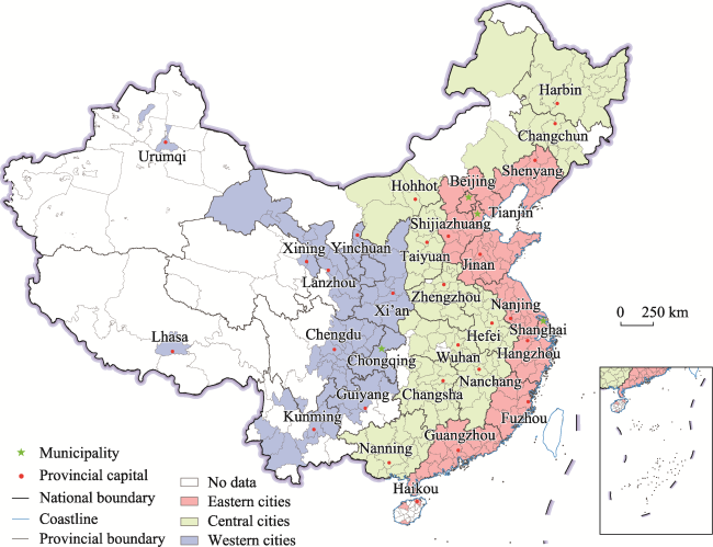
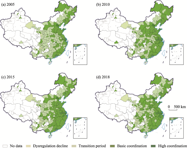
Urbanization interacts with land use through resource consumption and space encroachment. Clarifying the spatial correlations of the interactive relationship between urbanization and land use, along with their spatiotemporal dynamics, is of vital importance for addressing the complex interplay between urban development and land resources and identifying regional differences. However, previous studies have not sufficiently explored these issues. Herein, we introduce a coupling coordination degree (CCD) model and present the results of exploratory spatiotemporal analyses involving in-depth investigation of the CCD between urbanization quality and land-use intensity in 290 Chinese cities. The results demonstrate that the CCD for most cities was at the transition-period or basic-coordination stage. The dynamics of the spatial correlation of the CCD was found to increase from the east to the central and western regions, but this was found to decline overall. The movement direction and spatial dependence of the local spatial structure of the CCD exerted a dominant synergistic effect. The transition of the spatial correlation was mainly Type I (stable local and neighboring morphology), showing strong transfer inertia, path dependence, and locking features. Dynamic transitions occurred more in central and eastern cities. The results suggest that more cross-city cooperation could contribute to moderate land-resource exploitation for high-quality urbanization.

Cite this article

XU Feng , WANG Huan , ZUO Danyu , GONG Ziqiang . How does the coupling coordination relationship between high-quality urbanization and land use evolve in China? New evidence based on exploratory spatiotemporal analyses[J]. Journal of Geographical Sciences, 2024 , 34(5) : 871 -890 . DOI: 10.1007/s11442-024-2231-1

1 Introduction

Over the past century, urbanization has been one of the most spectacular scenes on our planet; however, the urbanization process leads to greater consumption of and higher pressure on land resources. If the demands on and encroachment into particular land resources exceed certain limits, the overall land-resource system will restrict the development of urbanization. Land-resource utilization, also called land use, refers not only to the different kinds of land coverage that are used for material production and environmental conservation but also to the scale and intensity of resource utilization for human activities (Han et al., 2021; Liu et al., 2023). Studies have highlighted the broader implications of land-use changes for economic and ecological security, examining the implications of the retention of or changes in land use for habitat, construction, farming, and biodiversity (Huang et al., 2015). Considering both natural and economic attributes, land use is increasingly being seen as both a driver and a consequence of urbanization (Song et al., 2018). Thus, understanding the reciprocal interacting core relationship between land-resource utilization and urbanization outcomes has attracted increasing attention from researchers.
Urbanization has become one of the most complex social and policy issues in post-industrial countries (Scott and Storper, 2015; Caldeira, 2017; Chen et al., 2021b). As the world’s largest developing country, China has built hundreds of cities, exhibiting the most remarkable urbanization of any country. The progress of urbanization was once evaluated from the perspectives of prosperity (Wong, 2015), quality of life (Morris, 2019), sustainability (Choon et al., 2011), and so on. In recent years, holistic approaches have been proposed when estimating the overall advancement of an urban system (Barnett and Parnell, 2016; Chen et al., 2021b; Pan et al., 2021a). Fundamentally, urbanization is a concept that considers the progress or retrogression of urban development; however, this occurs at the cost of the consumption of various resources, including land. Given the increasing pressures on resources and the environment, China has shifted to a new high-quality development model (Xu et al., 2023). With this new era of high-quality urbanization, the associated evaluation system should evolve, placing equal emphasis on the improvement of both quantity and quality. In practice, the targets of high-quality urbanization include a stronger and healthier economy, better public-service facilities, good eco-environmental protection, efficient resource utilization, and visionary resource reserves. None of these goals can be achieved without considering the capacity of land resources or the optimization of the land-use structure. Against such a background, the coupled relationship between land use and high-quality urbanization needs to be re-examined as urbanization increases.
With the shortage of land resources and the evolution of urbanization in China, academics have realized that the issues of land resources and urban development cannot be addressed by simply focusing on either individually, but they must be approached by clarifying the interaction mechanisms or coupling relationships between the two independent systems. A growing body of cross-city or -province observations has reported a significant association and even a heterogeneous relationship between land use and urbanization (Wang et al., 2018; Kuang et al., 2020). One recent investigation illustrated that urbanization outcomes associated with land use have high spatial heterogeneity (Xu et al., 2020). Previous research has demonstrated that simply making generalizations about the influence of land use on urbanization or vice versa is insufficient to reach complete conclusions regarding the interactive relationship between the two. More importantly, high-quality development requires the coordination of urbanization with land use to avoid overexploitation or insufficient utilization of land resources (Qu et al., 2023). Therefore, it is necessary to conduct a comprehensive analysis to understand the complex bidirectional development-resources relationship by undertaking more collaborative studies. As such, it appears that previous research is notably inadequate to address the current issues.
In terms of methods, studies on the interactions between environmental resources and urbanization initially used the environmental Kuznets curve (Wang et al., 2016). Then, others began to explore this relationship by focusing on intrinsic mechanisms and spatial variability (Kuang et al., 2020; Xu et al., 2023), or by using simulation techniques to predict future trends (Cui et al., 2020). Scholars have also studied the coupling relationships between urbanization and the environment (Fang et al., 2020). Regarding coupling relationships, the concept of “coupling” originates from physics, referring to the idea that two subsystems can affect each other through different interactions (Norgaard, 1990). Coupling coordination degree (CCD) models have been widely used to investigate the co-development status between social and natural subsystems (Lu et al., 2019; Zhang and Li, 2021). Specifically, the coupling degree can be used to measure the interrelations among different subsystems, and the coordination degree can be used to estimate the overall performance of a system with multiple compositions (Sun et al., 2024). Recently, some researchers have used CCD models to assess the interactive relationships between urbanization and land-use-induced changes or land-use-related phenomena, such as ecosystem services (Zhang et al., 2023), ecological-environmental status (Huang et al., 2020), and resource subsystems (Lu et al., 2019). Similarly, coupling mechanisms exist when identifying the interconnections between high-quality urban systems and land systems.
The simple identification of static two-way relationships is insufficient to reflect the connections, differences, and changing trends among regions. Thus, exploring the spatiotemporal dynamics and heterogeneities of spatial correlations in the bidirectional urbanization-resource relationship is extremely important to efforts to understand the land-use performance during urbanization at the local and regional levels. Moreover, evaluations from both the prefectural and dynamic perspectives can take into account geographical correlations and their spatiotemporal dynamics; this can help to improve the understandings of the harmonies and disharmonies among cities and any weaknesses or abnormalities in the land use of cities when pursuing high-quality urbanization.
Herein, we propose a framework for evaluating high-quality urbanization, introduce a land-use-intensity measure, apply a CCD model and undertake exploratory spatiotemporal analyses. The framework was used to examine the interrelationships between high-quality urbanization and land-use intensity in 290 Chinese cities from 2005 to 2018 and to identify spatial correlations and their spatiotemporal evolution. Our findings provide an empirical evidence for policymakers who wish to address resource mismatches for development, and also provide a reference for regional cooperation that facilitates efficient land use for urbanization.

2 Materials and methods

2.1 An evaluation framework for urbanization quality

2.1.1 Indicator selection

Reviewing the existing studies on urbanization, the dimensions and corresponding indicators of urbanization outcomes can be summarized as follows. Economic performance: Gross Domestic Product (GDP) (Jing et al., 2020), total import and export of goods (Kong et al., 2021), and the utilization of foreign capital (Zhang et al., 2022). Development potential: urbanization rate (Shen et al., 2012), science and technology expenditure (Shang et al., 2018), and population growth (Jing et al., 2020). Public services: residents’ pension insurance (Liu et al., 2023), healthcare (Yin et al., 2021), education (Li et al., 2020), and infrastructure (Chen et al., 2020). Ecological environment: waste discharge and recycling treatment (Wang et al., 2021), urban green space coverage (Pan et al., 2021b), and gas emissions (Chen et al., 2021b). Based on these indicators, this study established an evaluation framework for urbanization quality. This includes four target layers covering economic level, development potential, public services, and eco-environmental protection. Table 1 shows the details of 23 selected indicators that relate to economic progress, sustainable development, residents’ well-being, urban functions, and ecological environment.
Table 1 Comprehensive evaluation framework for urbanization quality
Target layer Indicator layer Illustration Unit
Economic level Economic production GDP/total population CNY
Enterprise profit Total profits of enterprise/GDP -
Employees’ salaries Actual total salaries paid to all employee/average number of employees CNY
Employment rate Urban registered unemployment rates %
Import and export of goods Total import and export of goods/GDP -
Foreign investment Total amount of foreign investment used/GDP -
Development potential Industrial structure Added value of tertiary industry/GDP %
Urbanization rate Urban population/total population %
Financial situation of industrial
enterprises
Current assets of industrial enterprises/(current assets + fixed assets) of industrial enterprises %
Science and technology expenditure Science and technology expenditure/Public budget expenditure %
Natural growth rate of population (Number of births − number of deaths)/average annual population
Deposit-to-loan ratio of financial
institutions
Total deposit balances of financial institutions/total loan balances of financial institutions -
Public
services
Internet popularity Internet users × 100/population household
Medical level Number of beds in hospitals and health centers × 10 000/population sheet
Public library collections Public library collections × 100/population piece
Road area Road coverage/total population m2
Student-teacher ratio in primary and secondary schools (Number of students/number of full-time teachers) in primary and secondary schools %
Urban pension insurance participants Number of urban employees participating in pension insurance/total population %
Ecological environment Green space coverage Green space coverage/built-up areas %
Industrial sulfur dioxide emissions Industrial sulfur dioxide emissions/GDP ton/million
Harmless treatment of garbage Harmless treatment of domestic garbage/amount of domestic waste %
Sewage centralized treatment Sewage treated in wastewater treatment plants/total amount of sewage %
PM2.5 concentration - µg/m3

2.1.2 Indicator weights

This study introduced an entropy method, which inherits the ideas of objective weighting, to define the indicator weights (Delgado and Romero, 2016). To begin with, we used min-max normalization to standardize the data into the range 0-1. The calculation of an indicator’s entropy value is as follows:
${{e}_{j}}=-k\sum\limits_{i=1}^{n}{{{P}_{ij}}}=-1/\ln (n)\sum\limits_{i=1}^{n}{\left( {{Z}_{ij}}/\sum\limits_{i=1}^{n}{{{Z}_{ij}}} \right)}$
where ej denotes the entropy value of the jth indicator, n is the number of samples, Pij is the sample weight, and Zij denotes the value of the jth indicator in the ith year. The indicator weight is then obtained using:
${{W}_{j}}={{d}_{j}}/\sum\limits_{i=1}^{n}{{{d}_{j}}}=(1-{{e}_{j}})/\sum\limits_{i=1}^{n}{(1-{{e}_{j}})}$
where Wj denotes the entropy weight of the jth indicator and dj is the variability coefficient of the jth indicator.

2.2 Methods

2.2.1 Land-use intensity

An evolving methodological tool now allows us to conceptualize and measure the aggregation level of a regional land system. The land-use intensity (LUI), an effective measure that is increasingly being used in land-related studies, provides a powerful tool for estimating the overall level of use of land resources; it relates to both the natural and economic attributes of a land system (Zhuang and Liu, 1997; Chen et al., 2021a). This composite index reflects not only the properties of the land system but also the effects on this system resulting from human activities and environmental changes (Xu and Chi, 2019). In the present approach, based on the land-classification system in China, 26 original land-use types are reclassified into just four (as shown in Table 2), and weightings are assigned according to the intensity of the involvement of human activity (Xu and Chi, 2019). The basic formula is:
${{L}_{d}}=100\times \sum\limits_{i=1}^{4}{{{A}_{i}}}\times {{C}_{i}}$
where Ld is the comprehensive index of land-use intensity within the study region, and Ai and Ci respectively denote the weighting and share of the area of the ith land-use type in the region. We multiply the index by 100 to facilitate subsequent calculation. Thus, the value of Ld falls within the range of 100-400; the larger the value, the higher the level of land-resource use and exploitation in the region.
Table 2 Classifications and weightings of land-use types
Classification Land-use type/weighting
Built-up land Urban land, rural settlements, land reclamation for new construction, and other built-up land/4
Agricultural production land Paddy field, dry land/3
Forest, grass, water, and other types of natural land Forest land, shrub land, sparse forest land, and other forest land; high-/medium-/low- coverage grassland; rivers, lakes, permanent glaciers, reservoirs, snow, beaches/2
Unused land Sand, gobi, salina, swampland, bare soil, bare rock, and others/1

2.2.2 CCD model

The CCD model is frequently applied to characterize adaptive relationships between objects (Li et al., 2012). In this model, the coupling degree indicates the strength of mutual influence and interaction among subsystems, and the coordination reveals the degree of regulation of subsystems or elements in an integrated and mutual whole. The CCD reflects the magnitude of benign coupling in an adaptive relation (Norgaard, 1990). The formulas for measuring the CCD are as follows:
$C=2\left\{ \left( {{U}_{1}}\times {{U}_{2}} \right) \right./\left( {{U}_{1}}+{{U}_{2}} \right){{\left. \left( {{U}_{1}}+{{U}_{2}} \right) \right\}}^{1/2}}$
$T=a{{U}_{1}}+b{{U}_{2}}$
$D={{\left( C\times T \right)}^{1/2}}$
where U1 and U2 represent the two subsystems; C denotes the coupling degree between these two subsystems; T denotes the comprehensive coordination index; D is the CCD; a and b are weights to be determined, and theoretically, a + b = 1. It is presupposed that urbanization and land-resource utilization are equally important; thus, for the purposes of this study, the coefficients a = b = 0.5. Following previous reports (Liu et al., 2018; Wang et al., 2022), the coupling degrees and CCDs are divided into four levels, the criteria for which are shown in Table 3.
Table 3 Classification of coupling degree and CCD
C value interval Coupling type D value interval Coupling coordination type
0.0 < C ≤ 0.3 Low-level coupling 0.0 < D ≤ 0.3 Dysregulation decline
0.3 < C ≤ 0.5 Antagonistic stage 0.3 < D ≤ 0.5 Transition period
0.5 < C ≤ 0.8 Run-in stage 0.5 < D ≤ 0.7 Basic coordination
0.8 < C ≤ 1.0 High-level coupling 0.7 < D ≤ 1.0 High coordination

2.2.3 Exploratory spatiotemporal analyses

Spatial autocorrelation statistics. Global spatial autocorrelation is frequently used to describe the spatial features of attribute values among regions. To estimate spatial correlations or differences, we introduce the Moran’s I spatial autocorrelation statistic. The global Moran’s I statistic indicates an average degree of differences between regions and their neighbors (Rey, 2001); it can be estimated as follows:
Moran’s I$=\frac{n\sum\limits_{i=1}^{n}{\sum\limits_{j=1}^{n}{{{W}_{ij}}\left( {{X}_{i}}-\overline{X} \right)\left( {{X}_{j}}-\overline{X} \right)}}}{\sum\limits_{i=1}^{n}{{{\left( {{X}_{i}}-\overline{X} \right)}^{2}}\left( \sum\limits_{i=1}^{n}{\sum\limits_{j=1}^{n}{{{W}_{ij}}}} \right)}}$
where n denotes the number of samples; Xi and Xj are the attribute values of samples i and j, respectively; and Wij represents the spatial weight matrix. The spatial weight is defined based on the distance between any two regions, known as the inverse-distance weight; this indicates that neighbors have greater spatial associations than regions that are farther apart (Shepard, 1968). The value of Moran’s I falls into the range [−1, 1]. Values of I > 0 indicate that a variable has a positive spatial correlation, and the larger the value the stronger the correlation; values of I < 0 indicate that a negative correlation exists among geographic units; if values of I = 0, this means that there is no spatial correlation.
The local indicator of spatial association (LISA) can better reflect the changing trends of local spatial differences (Anselin, 1995). The local Moran’s I statistic reveals the spatial autocorrelation from local perspective, and it can be estimated as follows:
${{I}_{i}}=\frac{n\left( {{X}_{i}}-\overline{X} \right)\sum\limits_{j=1}^{n}{{{W}_{ij}}{{\left( {{X}_{j}}-\overline{X} \right)}^{2}}}}{\sum\limits_{i=1}^{n}{{{\left( {{X}_{i}}-\overline{X} \right)}^{2}}}}$,
where Ii denotes the Moran’s I index, and the other variables have the same meanings as in Eq.(7).
Geometric features of the LISA time path. LISA and Moran scatter plots can be used together to detect spatial agglomeration and instability (Le Gallo and Ertur, 2003). By observing the length and angle of coordinates’ movement with time in the Moran scatter plot, we can connect these changes with the LISA time path to explain the spatiotemporal synergy or discretization of an object and to summarize the spatial connections of the objects from a dynamic perspective.
Specifically, the geometric characteristics of the LISA time path are defined in terms of relative length index Rli and curvature index Di (Murray et al., 2012). The relative length index Rli shows the dynamic characteristics of the local spatial structure of an object; a larger Rli value generally indicates a local spatial structure with stronger instability over time. The curvature index Di reflects the volatility of the local spatial structure in the spatial dimension; a larger Di value indicates a more curved movement of an object in the Moran scatter plot, indicating a more dynamic spatial dependence and a more fluctuating development process. The expressions for these values are as follows:
${{R}_{li}}=\frac{n\sum\limits_{t=1}^{T-1}{d\left( {{L}_{i,t}},{{L}_{i,t+1}} \right)}}{\sum\limits_{i=1}^{n}{\sum\limits_{t=1}^{T-1}{d\left( {{L}_{i,t}},{{L}_{i,t+1}} \right)}}}$
${{D}_{i}}=\frac{\sum\limits_{t=1}^{T-1}{d\left( {{L}_{i,t}},{{L}_{i,t+1}} \right)}}{d\left( {{L}_{i,t}},{{L}_{i,t+1}} \right)}$
where n is the number of samples, Li,t denotes the position of sample i in the Moran scatter plot in year t, d(Li,t, Li,t+1) denotes the distance over which sample i moves from year t to year t+1.
Movement direction of the LISA time path. To compare the movement angles of the objects in the Moran scatter plot, the movement direction of the LISA time path can be used to reveal the integrative characteristics of the spatial changes of objects and their geographic neighbors (Rey et al., 2011). The expression for this is as follows:
${{\theta }_{i}}=\arctan \frac{\sum\nolimits_{j}{\sin {{\theta }_{i}}}}{\sum\nolimits_{j}{\cos {{\theta }_{i}}}}$
The movement directions can be divided into four types, and their classifications and illustrations are listed in Table 4.
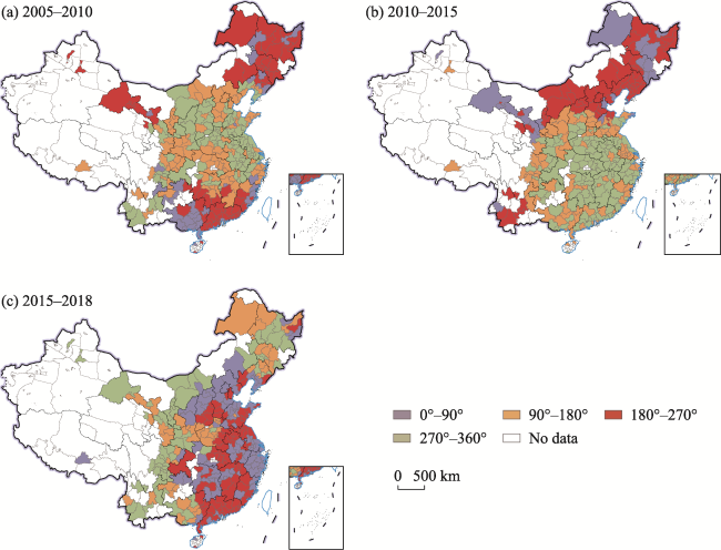
Table 4 Classifications and corresponding illustrations of LISA moving directions
θi Direction Illustrations
0°-90° Same direction High-high (HH) dynamic, showing a positive synergistic effect among the study object and its neighbors.
90°-180° Reverse Low-high (LH) dynamic, showing a reverse growth trend among the study object (lower) and its neighbors (higher).
180°-270° Same direction Low-low (LL) dynamic, showing a negative synergistic effect among the study object and its neighbors.
270°-360° Reverse High-low (HL) dynamic, showing a reverse growth trend among the study object
(higher) and its neighbors (lower).
Spatiotemporal transitions of LISA. We further estimate the spatiotemporal transitions of LISA based on its time path. These transitions embed the moving distance, direction, concentration degree, and other attributes of each spatial unit in a specific period into the Markov chain, revealing the temporal changes in local spatial correlations (Ye and Rey, 2013). The spatiotemporal transitions are classified into four main types, labelled I-IV (see Table 5). Type IV is further separated into two subtypes, Type IV(1) and Type IV(2), which respectively indicate local and neighboring transitions in the same and opposite directions (Jin et al., 2020).
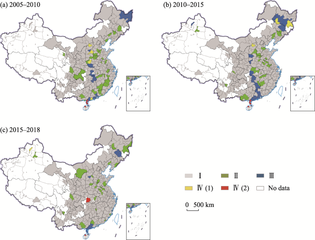
Table 5 Classifications and illustrations of spatiotemporal transition of LISA
Type Classification Transition illustrations
I HHt→HHt+1, HLt→HLt+1, LHt→LHt+1, LLt→LLt+1 Local and neighboring morphology is stable.
II HHt→LHt+1, HLt→LLt+1, LHt→HHt+1, LLt→HLt+1 Only local morphology is in transition.
III HHt→HLt+1, HLt→HHt+1, LHt→LLt+1, LLt→LHt+1 Only neighboring morphology is in transition.
IV(1) HHt→LLt+1, LLt→HHt+1 Local and neighboring transition in the same direction.
IV(2) HLt→LHt+1, LHt→HLt+1 Local and neighboring transition in opposite directions.

2.3 Data sources and preprocessing

The study area consisted of a total of 290 cities, comprising 4 centrally administrated municipalities, 27 provincial capital cities, and 259 prefecture-level cities in China (Figure 1). The study time points were at the ends of the years 2005, 2010, 2015, and 2018. The land-use datasets were obtained from the Resource and Environment Science and Data Center of the Chinese Academy of Sciences (https://www.resdc.cn/). The social, economic, and ecological data were collected from the China Urban Statistical Yearbook, provincial statistical yearbooks, urban statistical bulletins on national economic and social development, and official government websites. PM2.5 data were acquired using remote sensing measurements of aerosol optical depth. Some missing data were supplemented using an interpolation method, and all data were standardized to eliminate their dimensionality and make them comparable.
Figure 1 Scope of the study area in China

3 Results and discussion

3.1 Spatiotemporal characteristics of high-quality urbanization degree

As shown in Figure 2, the high-quality urbanization degree across the cities was found to show an upward trend over time, and it exhibited a spatial pattern that can be described as “higher in the eastern coast but lower in the central and western inland.” The relatively high values (orange and red) were primarily found in national or regional core cities such as Beijing, Shanghai, and Shenzhen, which have experienced rapid economic growth and have complete and advanced urbanization. The lowest-value cities, marked in blue, were mostly distributed in the central and western inland, and the northeast.
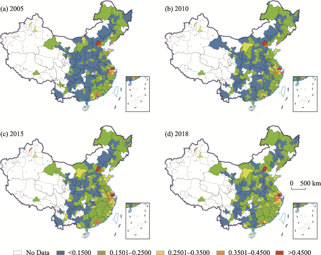
Figure 2 High-quality urbanization degrees of cities of China in 2005, 2010, 2015, and 2018
From a regional perspective, only Beijing, in the north region, remained at the highest level of urbanization quality, while Tianjin, Dalian, and Qingdao were in the relatively high-level range in some but not all years. In the south, Shenzhen, Shanghai, Zhuhai, and Suzhou performed best and stayed in the highest range, while Dongguan joined them in 2010. In 2018, Shenzhen and its neighboring cities, including Foshan, Guangzhou, and Dongguan, formed a cluster marked by high-quality urbanization. There was another city agglomeration located at the junction of three provincial administrations, Shanghai, Jiangsu (Suzhou and Wuxi), and Zhejiang (Jiaxing, Hangzhou, and Ningbo). Some central cities, such as Zhengzhou, Wuhan, Changsha, Nanchang, and some western cities, such as Chengdu, Chongqing, Karamay, Urumqi, also entered the medium range.
Almost no coastal cities remained at the lowest level of urbanization quality at the end of the study period; this was largely attributed to their better geographical locations and historical inertia of international economic cooperation. The rise of coastal cities has brought very large increases in economic productivity, strong development potential, and advanced governance abilities, thus forming regional medium- and high-value clusters. A small number of cities in the mid-west entered or even surpassed the medium level due to their economic strength, proven infrastructure, and outstanding specialized fields. It should be noted that most cities became stable high-quality urbanization poles due to their development inertia. However, some cities in the middle or high ranges experienced fluctuations or decline in their urbanization quality, demonstrating the potential risk of volatility and failure to achieve goals.

3.2 Spatiotemporal characteristics of CCD

The spatiotemporal distributions of the CCD between urbanization quality and land-use intensity at the four time points are shown in Figure 3. In general, the relationship was primarily in a transitional period or at a basic-coordination stage. The spatial pattern can be described as “higher in the east and lower in the west” at all stages. The number of cities at the high-coordination stage was small but increased year by year. The number of western cities at the dysregulation-decline stage was stable, while the number of cities at the transitional-period stage decreased.
Figure 3 Spatial patterns of urban CCD in China in 2005, 2010, 2015, and 2018
Cities in the eastern region, especially coastal ones, experienced higher CCD values than cities in other areas. The change from the transitional period to the basic-coordination stage was prominent for central cities. The gap of CCD narrowed within the neighbors in the east and central regions, and the trend of balance was spreading. The CCD values in the west were relatively poor. The number of western cities at the basic-coordination stage fluctuated over time, but that in the transition period decreased significantly. Generally, the average CCD values were higher in the east; this was followed by the central area, and the lowest values were found in the west. All exhibited a fluctuating but overall positive trend. Notably, the western region had a significant increase in CCD after some fluctuation.
It can be seen that, from a geographic perspective, the urbanization quality and land-use intensity in most eastern and central cities were mutually reinforcing at a high level: improving any aspect of urbanization can drive the growth of land use and exploitation, while tapping the land-use potential can provide sufficient resources for high-quality development of cities. Compared to mid-eastern regions, urbanization and land use in the west were undergoing a transition from dysregulation to coordinated development. However, a synchronized relationship between high-quality urbanization and land use had yet to be formed, and mutual constraints were more prominent. One explanation for this phenomenon was that inefficient land-use practices failed to cater to the development trend; in summary, high-quality urbanization was achieved by intensifying the land use. Another possible explanation is that either the efforts to shift a city’s development into a high-quality model did not work or the pursuit to create appropriate demands on land resources failed, resulting in a consistently low land-use intensity.

3.3 Spatiotemporal dynamics of CCD

3.3.1 Global spatial autocorrelation

The results of the global spatial autocorrelation of CCD between urbanization quality and land-use intensity are shown in Table 6. Moran’s I index passed the significance test in all years, and the coefficients were all positive, indicating that the CCD showed a positive autocorrelation effect. Temporally, the Moran’s I index has an inverted U-shape, indicating that the spatial autocorrelation of the coupling coordination relationship manifested as growth followed by a decline, reaching its peak in 2015.
Table 6 Moran’s I index of the CCD between urbanization quality and land-use intensity
Year Moran’s I Z P E(I) SD
2005 0.5746 14.7107 0.0010 −0.0035 0.0393
2010 0.5917 15.0086 0.0010 −0.0035 0.0394
2015 0.6104 15.9127 0.0010 −0.0035 0.0385
2018 0.5612 14.8387 0.0010 −0.0035 0.0380

3.3.2 Geometric features of the LISA time path

The results of the mean relative length index Rli (during four periods, 2005-2010, 2010- 2015, 2015-2018, and 2005-2018) and the curvature index Di (2005-2018 only) of the LISA time path in 31 provincial administrative regions are shown in Figure 4.
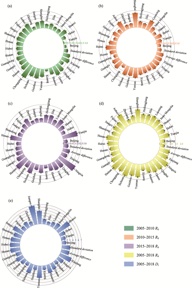
Figure 4 Relative length index (Rli) and curvature (Di) of the LISA time path in China
During the three time intervals, the proportion of provinces with higher mean Rli values than the national average decreased significantly, accounting for 51.61%, 48.39%, and 41.94% of the total. This indicates that the number of provinces that experienced bigger changes in the local spatial structure of their coupling coordination decreased, and the majority tended to be more stable. However, the spatial structure of the CCD in most western cities exhibited strong dynamic changes. The Rli values of several provinces, such as Chongqing and Guizhou, significantly fluctuated but decreased during the last period, stabilizing the spatial structure of the CCD. This could be because the relationship in western regions was initially poor, but some cities made progress in the adaptive relationship between urbanization and resource use, resulting in a significant improvement in the local spatial structure of the relationship.
The mean Rli values in Tianjin, Ningxia, Henan, and Inner Mongolia exhibited significant increases over time, indicating notable instability in the local spatial structure of the CCD. Conversely, the mean Rli values in Shandong, Jiangxi, and Shanghai demonstrated a continuous decrease over the three periods, and this was accompanied by increasing stability in their local spatial structures. For some cities, new progress or consolidation in terms of regulating the development-resources relationship and the triggering of changes in spatial correlations with their neighbors were thus identified.
From 2005 to 2018, low values of Rli were identified in Beijing, Hebei, Zhejiang, and Jiangsu, reflecting a generally stable local spatial structure and strong spatial dependency. The Rli values in central provinces, such as Henan, Hubei, and Anhui, exceeded the national average level, while the Rli values in the western provinces, such as Chongqing, Ningxia, Sichuan, and Yunnan, were also higher than the national average. In sum, the dynamic fluctuations in the spatial structure increased from the east to the central and western areas. Regarding Di, 20 provinces had lower values than the national average, accounting for 64.52% of the total. This indicates that the local spatial dependency of the CCD was mostly steady. Regions with higher Di values included: eastern provinces such as Jiangsu and Shanghai; central provinces like Shanxi, Hubei, Hunan, and Henan; and western provinces such as Xinjiang, Yunnan, Sichuan, and Shaanxi. In these regions, the local spatial dependency of the CCD between urbanization quality and land-use intensity fluctuated more, and the impacts from neighbors were more prominent. In other words, these cities had an inconsistent pace in terms of promoting urbanization and adjusting local-land use structures.

3.3.3 Movement direction of the LISA time path

The spatiotemporal dynamics of the local spatial autocorrelation of the CCD between urbanization quality and land-use intensity during the three periods, as indicated by the movement directions of the LISA time path, are shown in Figure 5. Overall, the major manifestation of the movement direction was a synergistic effect (0°-90° and 180°-270°), accounting for 59.66% or more. This shows a trend of spatial integration in the evolution of the local spatial correlation of the CCD. The numbers of cities that showed positive and negative synergistic effects were close. There were strong divergences and significant evolution of movement directions during different periods.
Figure 5 Movement directions of the LISA time path in China
During the time intervals 2005-2010 and 2010-2015, cities with positive synergistic effect (0°-90°) were predominantly concentrated in the mid-eastern region of China. From 2015 to 2018, cities exhibiting this trend were located in western regions, such as Ningxia, Shaanxi, Sichuan, and Chongqing, while those in eastern regions were concentrated in north Zhejiang and south Jiangsu. These places witnessed a growth of the CCD between urbanization and land use in both themselves and their neighbors. Cities with negative synergistic effects (180°-270°) were sporadically distributed throughout most provinces over time. Notably, some cities in Guangdong and Fujian underwent a significant change from negative to positive synergistic effect, and then back to negative.
Cities with the reverse growth trend in the local spatial effect of the CCD (90°-180° and 270°-360°) were scattered among the urban clusters with synergistic effects. Cities that showed an LH dynamic (90°-180°) were dispersed, while HL dynamic (270°-360°) cities had a wide dispersion but small agglomeration. During 2005-2010, LH and HL dynamic cities were observed in Hubei, Hunan, Chongqing, and then spreading to Guangxi, Gansu, Inner Mongolia, Heilongjiang, and Jilin during 2010-2015. During 2015-2018, these kinds of cities were sporadically identified in Anhui, Jiangxi, Jiangsu, and Shandong.
The divergence of movement directions between or within regions indicates that the positive synergistic effect drifted across cities with time. There were still numerous “blind areas” that failed to synchronously improve the development-resources relationship with their neighbors. This was possibly due to lagged development transformations or limitations in resource endowment. Hence, it is imperative to innovate a path that spreads positive effects by considering the roles of a city itself and inter-city forces. It is also crucial to make full use of the core and overflow cities that exert positive effects and to encourage the imitation of transformation actions and policy dividends.

3.3.4 Spatiotemporal transitions of LISA

The distribution of cities classified according to their spatiotemporal transitions in local spatial correlations of CCD is presented in Figure 6. Type I cities made up the overwhelming majority in all three periods. This suggests that most cities did not experience significant shifts, showing strong spatial cohesion and transition inertia in local spatial correlation. Types II and III cities were primarily observed in the central region. Some cities in Henan, Jiangxi, Hubei, Shaanxi, and Anhui experienced multiple changes in transition type between 2005 and 2018. Additionally, transition changes were found in the cities of Guangxi, Guangdong, Fujian, Liaoning, and Jilin provinces. All western cities, except for Xining, Nanning, Hezhou, Mianyang, Deyang, and Urumqi, which exhibited Type II or III transition at certain periods, entered a Type I transition with strong overall stability.
Figure 6 Spatiotemporal transitions of LISA in China
Type IV was characterized by simultaneous transitions of a city and its neighbors, and a few cities were classified into Type IV(1) or Type IV(2). For instance, Jiujiang exhibited a Type IV(1) transition in two consecutive periods, while Nanning showed a continuous Type IV(2) transition. Moreover, Handan, Bozhou, Zhaoqing, and Shizuishan changed from a Type I transition to Type IV(1) one, whereas Heze and Qinzhou shifted from Type I to Type IV(2). The cities experiencing three different transition types in the three periods included Zhaoqing, Xinxiang, Anyang, Bozhou, Jinzhou, Benxi, and Heze.
Overall, the cities that witnessed significant spatiotemporal transitions were predominantly concentrated in the central region, which implies that the state of the local spatial correlation of the CCD was stagnant in other regions. The distribution of the cities showing different spatiotemporal transitions indicates the need for a regional cooperation mechanism. Such a mechanism could adjust the relationship between urbanization and resource use. For the areas with less dynamic transitions—such as the western region, where Type I predominated—it is urgent that core cities adjacent to the central region should take a leading role in adjusting the adaptive relationship. The focus should shift to cultivating Types II and IV(1) transition cities, stimulating the urbanization transition and its spillover effects, and promoting high-level coordinated development among neighbors.

3.4 Abnormalities of CCD and their causes

To deeply review the spatiotemporal changes in the CCD from 2005 to 2018, most cities in the high coordination stage witnessed simultaneous high urbanization quality and strong land-use intensity. A proportion of cities that stayed in the stage of dysregulation decline or transition during most time periods faced two different but abnormal situations: one is the greater performance of urbanization relying on a relatively low intensity of land use, and the other is a poor urbanization quality with excessive consumption of land resources. For the former, it can be seen that Jiayuguan, Jinchang, Lasha, and Bayan Nur demonstrated transition-period status, and Jiuquan stayed in the stage of dysregulation decline; however, although the urbanization quality of these five western cities remained high enough, their land-use intensity ranked quite low. This indicates that they achieved high-quality urbanization goals with low dependence on the land system, which to some extent reflects the advantage of resource-utilization efficiency. The formation of a development model with a low CCD but competitive outcomes can be attributed to both natural limitations and policy incentives. Each of these cities has a relatively singular functional orientation, having replaced land with other development resources. For the latter, typical representatives are some prefecture-level cities in Henan Province that rank in the front line of land-use intensity but show unsatisfactory development quality. Possible causes may include overly extensive development and a relatively high proportion of the lands that were developed for cultivation. Two kinds of cities with abnormalities in their CCDs fell into the Type I category of LISA spatiotemporal transitions during all years, demonstrating the uniqueness of their characteristics and the transition inertia of their local spatial correlations.
The above results can naturally extend to the discussion of the benefits and drawbacks of solely relying on the coordinative relationship. Cases of high-quality urbanization and land use that interrelate, promote, and coordinate with each other can be identified as far as possible using a CCD model. However, in a small number of cases, analytic results based on the CCD model may have some uncertainties, and the overreliance on mathematical comparisons when exploring interrelationships may result in some unnecessarily pessimistic predictions, such as in cases of high-quality development supported by efficient but low-intensity land use. Nevertheless, these cases do not represent the mainstream, and they only require careful filtering.

4 Conclusions and policy recommendations

4.1 Conclusions

The relationship between urbanization and land use is complicated. Our study improves the existing understanding by thoroughly analyzing the CCD between urbanization quality and land-use intensity, investigating the spatial correlations of this relationship, and identifying the spatiotemporal dynamics and regional heterogeneities in the correlations in 290 Chinese cities from 2005 to 2018. Our findings can be summarized as follows.
In terms of urbanization quality, the overall distribution for the cities examined can be spatially characterized as “higher on the eastern coast but lower in the central and western inland regions,” and generally increased with time. Higher values were found in cities with strong economic bases and better urban functions, such as Beijing, Shanghai, and Shenzhen. High-quality urbanization across China can be easily recognized to a “polarization” phenomenon, and its volatility as well as the increasing disparities among cities became more prominent.
In terms of coupling coordination, most cities were at the transitional or basic-coordination stage. The averaged CCD values in the central and eastern cities were greater than for the western cities, but they generally continued to increase. Some municipalities, such as Beijing and Shanghai and non-capital cities such as Suzhou and Shenzhen, have more competitive advantages and strengths, so they presented better CCD values between urbanization and land use. However, some cities with abnormalities of CCD were also recognized as having inefficient use of or low dependence upon land resources when pursuing high-quality urbanization.
In terms of spatiality, the Moran’s I index of the CCD showed an inverted U-shape temporally. The geometric features of the LISA time path indicate that the overall stability of the local spatial correlation of the CCD was gradually increasing. The spatial structure of the correlations exhibited a stronger dynamic change in the west. The movement direction of the local spatial change and dependence was dominated by a synergistic effect. Cities that experienced HL or LH dynamics were widely distributed but had low levels of agglomeration.
In terms of spatial dynamics, most cities did not undergo significant spatiotemporal transitions in LISA, indicating the spatial cohesion and transition inertia in the local spatial correlations. The existence of path dependence and locking features in spatial correlations were confirmed. Some central cities experienced a significant transition, demonstrating weak local spatial correlations of CCD. Efforts should be made to encourage Types II and IV(1) transition cities to transform their development modes and stimulate positive spillover effects. Coordinated development should be promoted by implementing regional cooperation policies.

4.2 Policy recommendations

Regional differences were the most salient feature when observing the interrelationship between urban development and land use (Wei et al., 2017). The features identified in this study can help to adjust the development-resource relationships in cities and regions under the context of high-quality urbanization. Targeted policies can be formulated to establish a transmission mechanism for a high-level coupling coordination relationship between central and western cities. Effective experience and policies to support efficient use of land resources for high-quality urbanization should be publicized and applied via a regional cooperation mechanism.
For cities with stronger spatial associations and greater spatiotemporal dynamics in their associations, it is urgent to reach an agreement on the bidirectional and synchronous adjustment of urbanization targets and the resource-carrying capacity levels of surrounding cities. Because cities are at diverse development stages, the goals of high-quality urbanization should also be different. Excessive pursuit of multidimensional prosperity for a city is equally unprofitable to the over-exploitation of land resources, especially in ecologically fragile areas. It is also crucial to address the stagnation of negative spatial associations. When promoting the land conservation and intensive land use, cities should avoid homogeneous competition of rapid urbanization and land resource exploitation as much as possible.

4.3 Limitations

Due to the limitations in terms of variable selection and data acquisition, this study only conducted exploration of the relationship between urbanization and land use by focusing on their coupling coordination relationship. The drawbacks of using a CCD model for identifying intrinsic mechanisms should be addressed through other methods. Therefore, future studies should shift to examining the influence mechanisms of resource-driven urbanization by introducing spatial modelling methods and more in-depth analyses.
[1]
Anselin L, 1995. Local indicators of spatial association-LISA. Geographical Analysis, 27(2): 93-115.

[2]
Barnett C, Parnell S, 2016. Ideas, implementation and indicators: Epistemologies of the post-2015 urban agenda. Environment and Urbanization, 28(1): 87-98.

[3]
Caldeira T P R, 2017. Peripheral urbanization: Autoconstruction, transversal logics, and politics in cities of the global south. Environment and Planning D: Society & Space, 35(1): 3-20.

[4]
Chen L G, Yang X Y, Li L, et al., 2021a. The natural and socioeconomic influences on land-use intensity: Evidence from China. Land, 10(11): 1254.

[5]
Chen M X, Xian Y, Wang P L, et al., 2021b. Climate change and multi-dimensional sustainable urbanization. Journal of Geographical Sciences, 31(9): 1328-1348.

[6]
Chen Y, Zhu M K, Lu J L, et al., 2020. Evaluation of ecological city and analysis of obstacle factors under the background of high-quality development: Taking cities in the Yellow River Basin as examples. Ecological Indicators, 118: 106771.

[7]
Choon S, Siwar C, Pereira J J,et al., 2011. A sustainable city index for Malaysia. International Journal of Sustainable Development & World Ecology, 18(1): 28-35.

[8]
Cui X G, Fang C L, Liu H M, et al., 2020. Dynamic simulation of urbanization and eco-environment coupling: Current knowledge and future prospects. Journal of Geographical Sciences, 30(12): 333-352.

[9]
Delgado A, Romero I, 2016. Environmental conflict analysis using an integrated grey clustering and entropy-weight method: A case study of a mining project in Peru. Environmental Modelling & Software, 77: 108-121.

[10]
Fang C L, Cui X G, Deng X Z, et al., 2020. Urbanization and eco-environment coupling circle theory and coupler regulation. Journal of Geographical Sciences, 30(7): 1043-1059.

DOI

[11]
Han H, Guo L, Zhang J Q, et al. 2021. Spatiotemporal analysis of the coordination of economic development, resource utilization, and environmental quality in the Beijing-Tianjin-Hebei urban agglomeration. Ecological Indicators, 127: 107724.

[12]
Huang J C, Na Y, Guo Y, 2020. Spatiotemporal characteristics and driving mechanism of the coupling coordination degree of urbanization and ecological environment in Kazakhstan. Journal of Geographical Sciences, 30(11): 1802-1824.

DOI

[13]
Huang Z J, Wei Y H D, He C F, et al., 2015. Urban land expansion under economic transition in China: A multilevel modeling analysis. Habitat International, 47: 69-82.

[14]
Jin G, Deng X Z, Dong Y, et al., 2020. China’s multidimensional poverty measurement and its spatiotemporal interaction characteristics in the perspective of development geography. Acta Geographica Sinica, 75(8): 1633-1646. (in Chinese)

[15]
Jing C, Tao H, Jiang T et al., 2020. Population, urbanization and economic scenarios over the Belt and Road region under the Shared Socioeconomic Pathways. Journal of Geographical Sciences, 30(1): 68-84.

DOI

[16]
Kong Q X, Peng D, Ni Y H, et al., 2021. Trade openness and economic growth quality of China: Empirical analysis using ARDL model. Finance Research Letters, 38: 101488.

[17]
Kuang B, Lu X H, Han J, et al., 2020. How urbanization influence urban land consumption intensity: Evidence from China. Habitat International, 100: 102103.

[18]
Le Gallo J, Ertur C, 2003. Exploratory spatial data analysis of the distribution of regional per capita GDP in Europe, 1980-1995. Papers in Regional Science, 82(2): 175-201.

[19]
Li W W, Yi P T, Zhang D N, et al. 2020. Assessment of coordinated development between social economy and ecological environment: Case study of resource-based cities in northeastern China. Sustainable Cities and Society, 59: 102208.

[20]
Li Y F, Li Y, Zhou Y, et al., 2012. Investigation of a coupling model of coordination between urbanization and the environment. Journal of Environmental Management, 98: 127-133.

DOI PMID

[21]
Liu N N, Liu C Z, Xia Y F, et al., 2018. Examining the coordination between urbanization and eco-environment using coupling and spatial analyses: A case study in China. Ecological Indicators, 93: 1163-1175.

[22]
Liu Y B, Lu F, Xian C F, et al., 2023. Urban development and resource endowments shape natural resource utilization efficiency in Chinese cities. Journal of Environmental Sciences, 126: 806-816.

DOI PMID

[23]
Lu X, Xue M G, Hu M S, 2019. Dynamic simulation and assessment of the coupling coordination degree of the economy-resource-environment system: Case of Wuhan city in China. Journal of Environmental Management, 230: 474-487.

DOI PMID

[24]
Morris E A, 2019. Do cities or suburbs offer higher quality of life? Intrametropolitan location, activity patterns, access, and subjective well-being. Cities, 89: 228-242.

DOI

[25]
Murray A T, Liu Y, Rey S J, et al., 2012. Exploring movement object patterns. The Annals of Regional Science, 49(2): 471-484.

[26]
Norgaard R B, 1990. Economic indicators of resource scarcity: A critical essay. Journal of Environmental Economics and Management, 19(1): 19-25.

[27]
Pan W, Wang J, Lu Z, et al., 2021a. High-quality development in China: Measurement system, spatial pattern, and improvement paths. Habitat International, 118: 102458.

[28]
Pan Y X, Zhang B Y, Wu Y, et al., 2021b. Sustainability assessment of urban ecological-economic systems based on emergy analysis: A case study in Simao, China. Ecological Indicators, 121: 107157.

[29]
Qu Y B, Zhang Y J, Wang S L, et al., 2023. Coordinated development of land multi-function space: An analytical framework for matching the supply of resources and environment with the use of land space for ecological protection, agricultural production and urban construction. Journal of Geographical Sciences, 33(2): 311-339.

DOI

[30]
Rey S J, 2001. Spatial empirics for economic growth and convergence. Geographical Analysis, 33(3): 195-214.

[31]
Rey S J, Murray A T, Anselin L, 2011. Visualizing regional income distribution dynamics. Letters in Spatial and Resource Sciences, 4(1): 81-90.

[32]
Scott A J, Storper M, 2015. The nature of cities: The scope and limits of urban theory. International Journal of Urban and Regional Research, 39(1): 1-15.

[33]
Shang J, Wang Z, Li L, Chen Y, et al., 2018. A study on the correlation between technology innovation and the new-type urbanization in Shaanxi province. Technological Forecasting and Social Change, 135: 266-273.

[34]
Shen L Y, Peng Y, Zhang X L, et al. 2012. An alternative model for evaluating sustainable urbanization. Cities, 29(1): 32-39.

[35]
Shepard D, 1968. A two-dimensional interpolation function for irregularly spaced data. In: Proceedings of the 1968 23rd ACM National Conference. New York: ACM, 517-524.

[36]
Song X P, Hansen M C, Stehman S V et al., 2018. Global land change from 1982 to 2016. Nature, 560: 639-643.

[37]
Sun K, Han J M, Wu Q R et al., 2024. The coupling coordination and spatiotemporal evolution of industrial water-energy-CO2 in the Yellow River Basin. Science of the Total Environment, 912: 169012.

[38]
Wang J, Lin Y F, Glendinning A, Xu Y Q, 2018. Land-use changes and land policies evolution in China’s urbanization. Land Use Policy, 75: 375-387.

[39]
Wang S J, Cui Z T, Lin J J, et al., 2022. The coupling relationship between urbanization and ecological resilience in the Pearl River Delta. Journal of Geographical Sciences, 32(1): 44-64.

DOI

[40]
Wang Y N, Fang X L, Yin S W, et al., 2021. Low-carbon development quality of cities in China: Evaluation and obstacle analysis. Sustainable Cities and Society, 64: 102553.

[41]
Wang Z H, Bao Y H, Wen Z G, et al., 2016. Analysis of relationship between Beijing’s environment and development based on Environmental Kuznets Curve. Ecological Indicators, 67: 474-483.

[42]
Wei Y H D, Li H, Yue W Z, 2017. Urban land expansion and regional inequality in transitional China. Landscape and Urban Planning, 163: 17-31.

[43]
Wong C, 2015. A framework for ‘City Prosperity Index’: Linking indicators, analysis and policy. Habitat International, 45: 3-9.

[44]
Xu F, Chi G Q, 2019. Spatiotemporal variations of land use intensity and its driving forces in China, 2000-2010. Regional Environmental Change, 19: 2583-2596.

[45]
Xu F, Chi G Q, Zhang Z X, et al. 2023. How does quality regional growth affect land resources dependence in China? Evidence based on spatial Durbin panel models. Resources Policy, 81: 103402.

[46]
Xu F, Wang Z Q, Chi G Q, et al., 2020. The impacts of population and agglomeration development on land use intensity: New evidence behind urbanization in China. Land Use Policy, 95: 104639.

[47]
Ye X Y, Rey S, 2013. A framework for exploratory space-time analysis of economic data. The Annals of Regional Science, 50: 315-339.

[48]
Yin J F, Liu H M, Shi P J, et al., 2021. Exploring coupling relationship between urban connection and high-quality development using the case of Lanzhou-Xining urban agglomeration. Complexity, 2021: 1-12.

[49]
Zhang F, Xu N, Wang C et al., 2023. Multi-scale coupling analysis of urbanization and ecosystem services supply-demand budget in the Beijing-Tianjin-Hebei region, China. Journal of Geographical Sciences, 33(2): 340-356.

DOI

[50]
Zhang F T, Tan H M, Zhao P et al., 2022. What was the spatiotemporal evolution characteristics of high-quality development in China? A case study of the Yangtze River economic belt based on the ICGOS-SBM model. Ecological Indicators, 145: 109593.

[51]
Zhang T, Li L, 2021. Research on temporal and spatial variations in the degree of coupling coordination of tourism-urbanization-ecological environment: A case study of Heilongjiang, China. Environment Development and Sustainability, 23: 8474-8491.

[52]
Zhuang D F, Liu J Y, 1997. Modeling of regional differentiation of land-use degree in China. Chinese Geographical Science, 7(4): 302-309. (in Chinese)

Outlines

/