
Journal of Geographical Sciences >
Understanding coordinated development through spatial structure and network robustness: A case study of the Beijing-Tianjin-Hebei region
|
Wang Hao (1985-), PhD, specialized in territorial spatial planning and urban physical examination. E-mail: wanghao@casm.ac.cn |
Received date: 2023-07-29
Accepted date: 2024-03-05
Online published: 2024-05-31
Supported by
National Key Research and Development Program(2023YFC3804001)
Natural Resources Planning and Management Project(A2417)
Natural Resources Planning and Management Project(A2418)
In the context of accelerated globalization, intercity factor flows are becoming increasingly dependent on a reasonable and orderly spatial structure. Therefore, an in-depth study of the optimization and adjustment of spatial structure is essential for coordinated development. This study quantitatively evaluated urban development levels and introduced network analysis methods to analyse the spatial structure and robustness of development. The results indicated the following: (1) The urban development level in the Beijing-Tianjin- Hebei (BTH) region increased in all dimensions, and the transmission efficiency significantly improved. (2) The spatial structure of the BTH region has been relatively stable, as illustrated by the main pattern of the spatial distribution of central cities, with a trend towards contiguous development. (3) The ranking of network robustness is environment>society>economy, and the core network and key nodes are primarily located within the radiation of the three central cities of Beijing, Tianjin, and Shijiazhuang. (4) The coordinated development of the BTH region is effective but still needs to be optimized and adjusted, and the strategic significance of edge cities has not been completely exploited. This study aims to provide an emerging analytical perspective for optimizing regional spatial structure and promoting regional coordinated development.
WANG Hao , ZHANG Xiaoyuan , ZHANG Xiaoyu , LIU Ruowen , NING Xiaogang . Understanding coordinated development through spatial structure and network robustness: A case study of the Beijing-Tianjin-Hebei region[J]. Journal of Geographical Sciences, 2024 , 34(5) : 1007 -1036 . DOI: 10.1007/s11442-024-2237-8
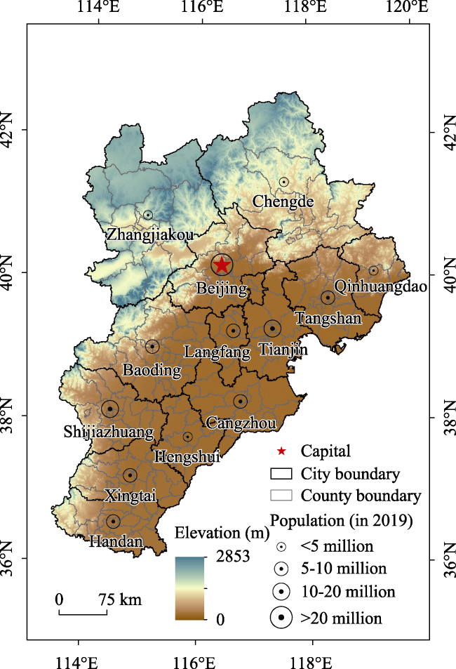
Figure 1 Location of the study area (Beijing-Tianjin-Hebei region) |
Table 1 Research data sources and description |
| Name | Data source | Resolution | Brief description |
|---|---|---|---|
| Land use data | Geographic Condition Monitoring Data | 2 m/yearly | Reflection of the actual development and construction of the urban area |
| Road network data | Geographic Condition Monitoring Data, OpenStreetMap dataset (https://www.openstreetmap.org/) | 2 m/yearly | Quantification of the urban transportation development level |
| POI data | Geographic Condition Monitoring Data, POI data (https://www.amap.com/) | 2 m/yearly | Indication of people’s living standards |
| Social and economic data | Beijing Regional Statistics Yearbook, Tianjin Statistical Yearbook, and Hebei Statistical Yearbook | Quantitative measurement of quality in all aspects of the city | |
| PM2.5 data | ChinaHighPM2.5 (https://doi.org/10.5281/zenodo.6398971) | 1 km/yearly | Characterization of the regional environmental conditions |
| Nighttime light data | EOG Group, Colorado School of Mines, USA (https://eogdata.mines.edu/products/vnl/) | 500 m/yearly | Characterization of the regional economic development level |
| Remote sensing image | Landsat8 OLI (https://earthengine.google.com/) | 30 m/yearly | Quantification of urban environmental quality |
| Administrative boundary | National Basic Geographic Information Database (https://www.resdc.cn) | / | Definition of the scope of the study area |
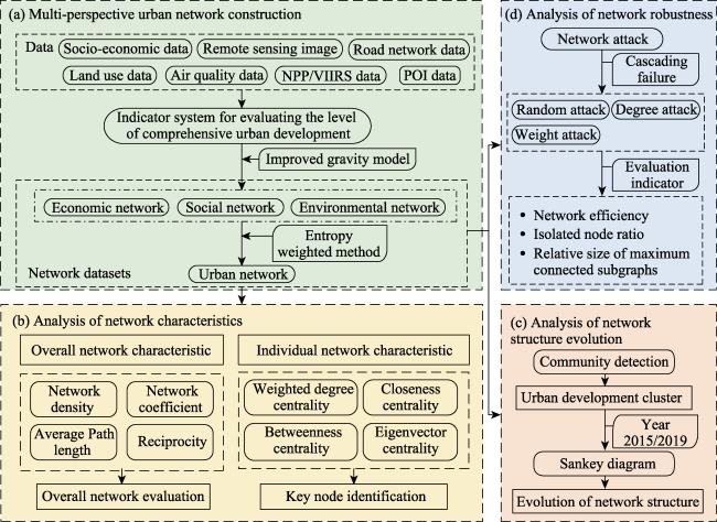
Figure 2 Research framework |
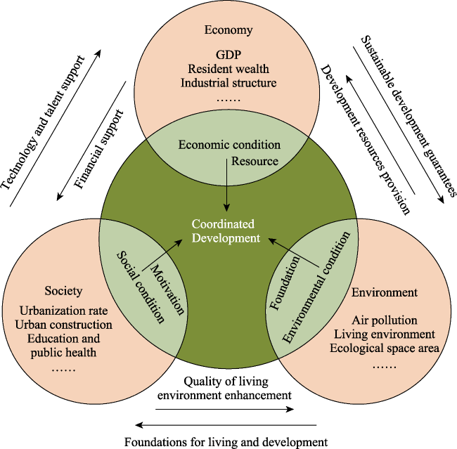
Figure 3 Interaction of the social, economic and environmental subsystems |
Table 2 The indicator system for evaluating the comprehensive development level of the ESE of cities |
| Guideline layer | Indicator layer & indicator type | Unit | Indicator meaning | Weight |
|---|---|---|---|---|
| Economy (ECO) | GDP (+) | 109 Yuan | Regional economic power | 0.2186 |
| The percentage of added value of the tertiary industry of GDP (+) | % | Industrial and economic structure | 0.0341 | |
| per capita GDP (+) | 104 yuan | Residents’ living standards | 0.0873 | |
| The averages NTL data (+) | / | Economic development level | 0.2282 | |
| General public budget revenues (+) | 104 yuan | Regional financial strength | 0.2354 | |
| General public budget expenditure (+) | 104 yuan | Regional financial strength | 0.1679 | |
| Disposable income per urban resident (+) | yuan | Residents’ living standards | 0.0285 | |
| Society (SCO) | Road network density (+) | km/km² | Infrastructure level | 0.1325 |
| Urbanization rate (+) | % | Urban development potential | 0.0202 | |
| Population density (+) | people/km2 | Population growth potential | 0.2097 | |
| Length of road per capita (+) | m/people | Convenience of transportation | 0.1583 | |
| Percentage of built-up area (+) | % | Land development intensity | 0.0548 | |
| Number of health facilities per 10,000 people (+) | Institute/104 people | Health services level | 0.0344 | |
| Number of schools per 10,000 people (+) | Institute/104 people | Education level | 0.0455 | |
| Open space area per capita (+) | people/km² | Population’s standard of living | 0.3446 | |
| Environment (ENT) | PM2.5 concentration in the air (-) | μg/m3 | Air quality levels | 0.1837 |
| Percentage of Ecological space area (+) | % | Environmental quality levels | 0.5204 | |
| NDVI (+) | / | Urban greenness | 0.1050 | |
| LST (-) | / | Urban heat | 0.0312 | |
| WET (+) | / | Urban humidity | 0.1597 |
Table 3 Overall and individual network indicators |
| Indicator name | Description | Equation | ||
|---|---|---|---|---|
| Network density (D) | Refers to the degree of correlation between network nodes, i.e., the probability of connection between nodes. | $D\text{=}\frac{l}{n\left( n-1 \right)}$ (3) | ||
| Average path length (L) | Measures the level of network reachability and the average distance between nodes. | $L=\frac{2}{n\left( n-1 \right)}\sum\limits_{i\ne j}{{{d}_{ij}}}$ (4) | ||
| Average clustering coefficient (C) | Indicates the degree of node aggregation in the network and enables the calculation of the probability that two neighbours of a node may be connected to each other. | $C=\frac{1}{n}\sum\limits_{i\in n}{\frac{2{{m}_{i}}}{{{k}_{i}}\left( {{k}_{i}}-1 \right)}}$ (5) | ||
| Reciprocity (R) | The ratio of bidirectionally connected edges to all edges in a directed weighted network (Garlaschelli and Loffredo, 2004) and is able to measure the closeness of the interaction between two nodes. | $R=\frac{{{L}_{bi}}}{{{L}_{bi}}+{{L}_{uni}}}$ (6) | ||
| Degree centrality (DC) | Measures a node’s connectivity and influence, differentiating between its ability to receive and exert influence in directed networks. | $D{{C}_{i}}=\sum\limits_{j=1}^{n}{{{a}_{ji}}{{w}_{ji}}}+\sum\limits_{j=1}^{n}{{{a}_{ij}}{{w}_{ij}}}$ (7) | ||
| Closeness centrality (CC) | Characterizes the correlation between a city’s development and that of other cities, demonstrates superior efficiency of external interactions in regional development networks. | $C{{C}_{i}}=\frac{n-1}{\sum\nolimits_{j\ne i}^{n}{{{d}^{w}}\left( i,j \right)}}$ (8) | ||
| Betweenness centrality (BC) | Reflects the ability of cities to play a communicative and coordinating role in regional development, and to control or influence the flow of resources and information. | $B{{C}_{i}}=\frac{2}{(n-1)(n-2)}\sum\limits_{j<k}^{n}{\frac{{{N}_{jk}}\left( i \right)}{{{N}_{jk}}}}$(9) | ||
| Eigenvector centrality (EC) | Reflects the degree to which the urban entity itself is connected to key nodes in the vicinity (Li et al., 2016), demonstrating the centrality of the nodes | $E{{C}_{i}}={{\lambda }^{-1}}\sum\limits_{j=1}^{n}{{{a}_{ij}}{{x}_{ij}}}$ (10) | ||
Table 4 Network robustness evaluation indicator system |
| Indicator name | Description | Equation |
|---|---|---|
| Network efficiency | Reflects the ease of network operation, the more efficient the network, the better the network connectivity | $E=\frac{1}{n\left( n-1 \right)}\sum\limits_{i=1}^{n}{\sum\limits_{j=1\left( i\ne j \right)}^{n}{{{H}_{ij}}}}$ (12) |
| Isolated node ratio | Reflects the proportion of nodes that have no edges connected to them when the network is under attack | $\Delta N=\left( 1-\frac{{{n}^{*}}}{n} \right)*100%$ (13) |
| Relative size of maximum connected subgraphs | Reflects the size of the largest subgraph during network fragmentation in the event of an attack, providing a visual representation of the extent of network disruption | $G=\frac{{{P}^{*}}}{P}$ (14) |
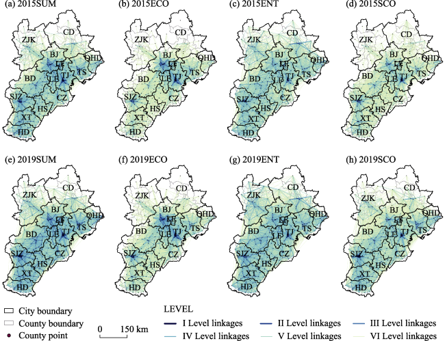
Figure 4 Evolution of various networks in the Beijing-Tianjin-Hebei region from 2015-2019 |
Table 5 Overall network structure characteristics |
| Name | 2015ENT | 2019ENT | 2015ECO | 2019ECO | 2015SCO | 2019SCO | 2015SUM | 2019SUM |
|---|---|---|---|---|---|---|---|---|
| D | 0.503 | 0.609 | 0.416 | 0.562 | 0.483 | 0.719 | 0.514 | 0.642 |
| L | 1.558 | 1.416 | 1.686 | 1.467 | 1.582 | 1.283 | 1.548 | 1.373 |
| C | 0.765 | 0.801 | 0.719 | 0.778 | 0.754 | 0.844 | 0.777 | 0.826 |
| R | 0.830 | 0.861 | 0.598 | 0.693 | 0.692 | 0.804 | 0.839 | 0.902 |
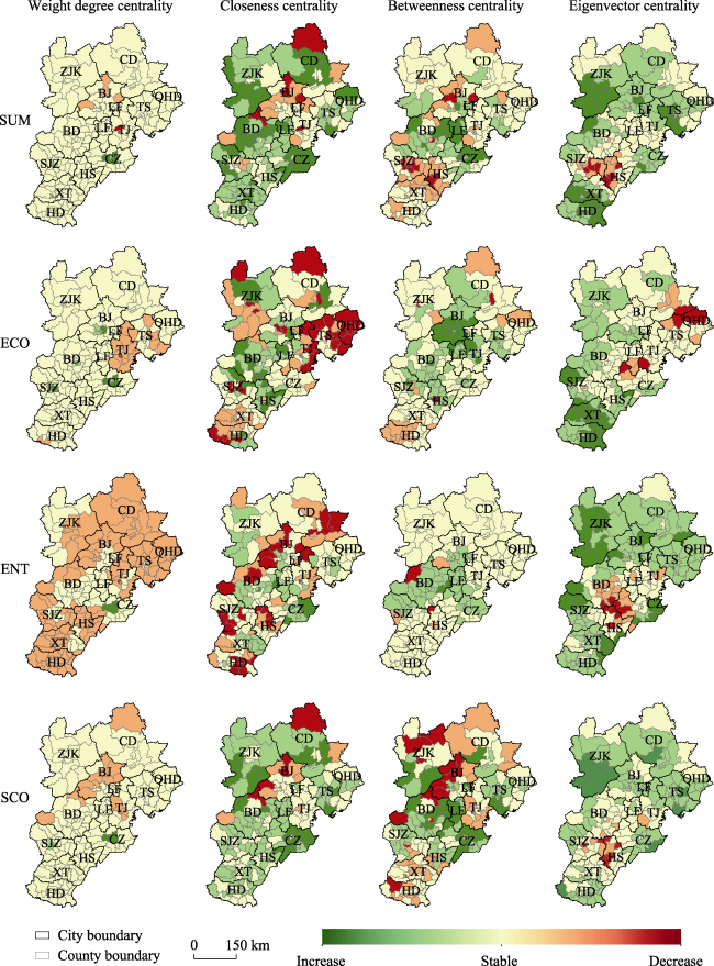
Figure 5 Network centrality differences among different subsystems in the Beijing-Tianjin-Hebei region from 2015 to 2019 |
Figure 6 Evolution of various networks in the Beijing-Tianjin-Hebei region from 2015-2019 (Note: Different colours represent different clusters, and the width size represents the number of city transfers.) |
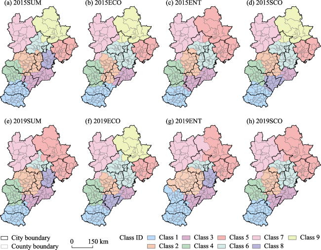
Figure 7 Results of city clustering in different dimensions in the Beijing-Tianjin-Hebei region from 2015-2019 (Note: Different classes represent different urban clusters.) |
Figure 8 Variations in network robustness characteristic value under different node attack methods |
Figure 9 Multidimensional core network in the Beijing-Tianjin-Hebei region (Note: Different levels represent the contact strength, where the first level is the highest; the grading criteria are the same as those in Figure 4.) |
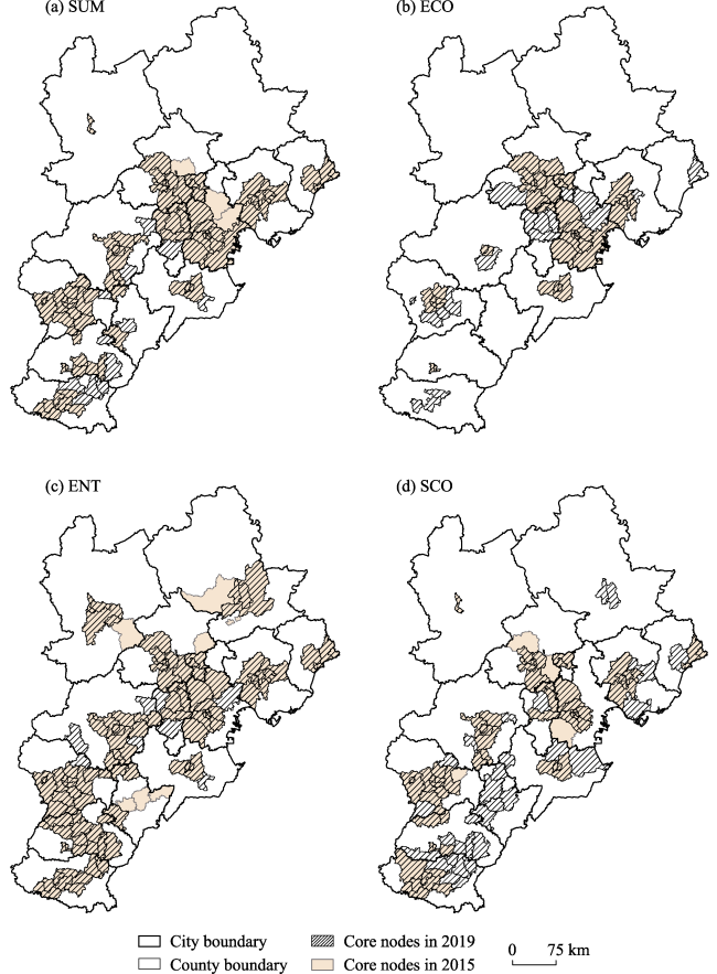
Figure 10 Core nodes of the multidimensional network in the Beijing-Tianjin-Hebei region at county level |
| [1] |
|
| [2] |
|
| [3] |
|
| [4] |
|
| [5] |
|
| [6] |
|
| [7] |
|
| [8] |
|
| [9] |
|
| [10] |
|
| [11] |
|
| [12] |
|
| [13] |
|
| [14] |
|
| [15] |
|
| [16] |
|
| [17] |
|
| [18] |
|
| [19] |
|
| [20] |
|
| [21] |
|
| [22] |
|
| [23] |
|
| [24] |
|
| [25] |
|
| [26] |
|
| [27] |
|
| [28] |
|
| [29] |
|
| [30] |
|
| [31] |
|
| [32] |
|
| [33] |
|
| [34] |
|
| [35] |
|
| [36] |
|
| [37] |
|
| [38] |
|
| [39] |
|
| [40] |
|
| [41] |
|
| [42] |
|
| [43] |
|
| [44] |
|
| [45] |
|
| [46] |
|
| [47] |
|
| [48] |
|
| [49] |
|
| [50] |
|
| [51] |
|
| [52] |
|
| [53] |
|
| [54] |
|
| [55] |
|
| [56] |
|
| [57] |
|
| [58] |
|
| [59] |
|
| [60] |
|
| [61] |
|
| [62] |
|
| [63] |
|
| [64] |
|
| [65] |
|
| [66] |
|
| [67] |
|
| [68] |
|
| [69] |
|
| [70] |
|
| [71] |
|
| [72] |
|
| [73] |
|
| [74] |
|
| [75] |
|
| [76] |
|
| [77] |
|
| [78] |
|
| [79] |
|
| [80] |
|
| [81] |
|
| [82] |
|
| [83] |
|
| [84] |
|
| [85] |
|
| [86] |
|
| [87] |
|
| [88] |
|
| [89] |
|
| [90] |
|
| [91] |
|
| [92] |
|
| [93] |
|
| [94] |
|
| [95] |
|
| [96] |
|
| [97] |
|
| [98] |
|
| [99] |
|
| [100] |
|
| [101] |
|
| [102] |
|
/
| 〈 |
|
〉 |


