Research Articles

Temporal and spatial laws and simulations of erosion and deposition in the Lower Yellow River since the operation of the Xiaolangdi Reservoir

  • SHEN Yi , 1, 2, 3 ,
  • WU Baosheng , 1, 2, 3, * ,
  • WANG Yanjun 4 ,
  • QIN Chao 1, 2, 3 ,
  • ZHENG Shan 5
Expand
  • 1. State Key Laboratory of Hydroscience and Engineering, Tsinghua University, Beijing 100084, China
  • 2. Key Laboratory of Hydrosphere Sciences of the Ministry of Water Resources, Tsinghua University, Beijing 100084, China
  • 3. Department of Hydraulic Engineering, Tsinghua University, Beijing 100084, China
  • 4. Key Laboratory of River Regulation and Flood Control of Ministry of Water Resources, Yangtze River Scientific Research Institute, Wuhan 430010, China
  • 5. State Key Laboratory of Water Resources and Hydropower Engineering Science, Wuhan University, Wuhan 430072, China
*Wu Baosheng, PhD and Professor, specialized in hydraulics and river dynamics. E-mail:

Shen Yi, PhD Candidate, specialized in fluvial processes. E-mail:

Received date: 2023-12-07

  Accepted date: 2024-01-20

  Online published: 2024-04-24

Supported by

National Natural Science Foundation of China(U2243218)

Abstract

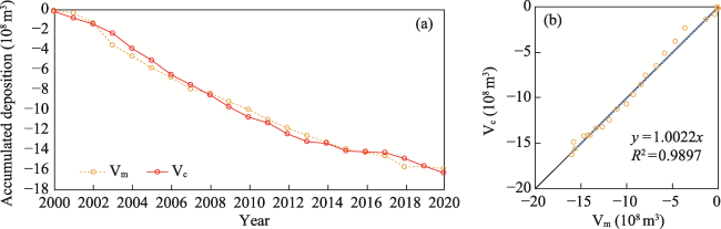
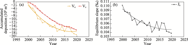
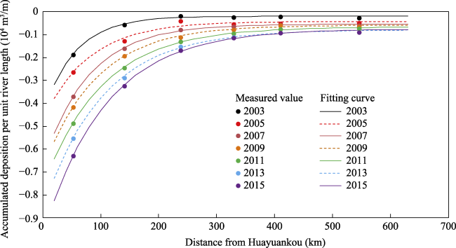
This study focuses on the Lower Yellow River (LYR), which has experienced continuous erosion since the operation of Xiaolangdi Reservoir in 1999, and its spatiotemporal variation process is complex. Based on the single-step mode of the Delayed Response Model (DRM), we proposed a calculation method for simulating the accumulated erosion and deposition volume in the LYR. The coefficient of determination R2 between the calculated and measured values from 2000 to 2020 is 0.99. Currently, the LYR is undergoing continuous erosion, however the erosion rate is gradually slowing down, and the difference between the equilibrium and calculated values of accumulated erosion and deposition volume gradually decreases, which means riverbed erosion has a tendency towards equilibrium. Additionally, we derive a formula to simulate the spatial distribution of the main channel accumulated erosion volume per unit river length in the LYR based on the non-equilibrium suspended sediment transport equation. The coefficient of determination R2 between the fitted values and measured values from 2003 to 2015 is approximately 0.98-0.99, with a relative error of approximately 6.2%. The findings in this research suggest that under the current background of decreasing sediment inflow and continuous erosion in the LYR, it takes approximately 3.0 years for the riverbed to achieve half of the erosion and deposition adjustment and approximately 13.0 years to achieve 95% of the adjustment. Moreover, the spatial distribution of accumulated main channel erosion volume in the LYR tends to become uniform with the continuous development of erosion. These results could provide a valuable reference for analysing the complex spatiotemporal variation process in the LYR.

Cite this article

SHEN Yi , WU Baosheng , WANG Yanjun , QIN Chao , ZHENG Shan . Temporal and spatial laws and simulations of erosion and deposition in the Lower Yellow River since the operation of the Xiaolangdi Reservoir[J]. Journal of Geographical Sciences, 2024 , 34(3) : 591 -609 . DOI: 10.1007/s11442-024-2219-x

1 Introduction

Rivers are open systems with clear spatial boundaries which exchange material and energy with the outside world. As a medium for water and sediment transport, they transport water and sediment from the earth's surface to the ocean, playing an important role in shaping the earth's surface morphology (Knighton, 1998). With the downstream movement of water and sediment, the riverbed undergoes continuous erosion and sedimentation, manifested at the micro level as the gradual approach of sediment concentration to sediment transport capacity and at the macro level as the development of river channel morphology towards a certain hydraulic geometry (Qian et al., 1987; Wu and Zheng, 2015). As a result, rivers can approach a relatively equilibrium state over a long period. Generally, in the process of adjustment from the non-equilibrium state to the equilibrium state, the initial adjustment rate is relatively large. As the system gradually approaches the equilibrium state, the adjustment rate will decrease gradually. Furthermore, when the system approaches equilibrium infinitely, the adjustment rate approaches zero. This characteristic in the fluvial system can be represented by the rate law or exponential decay equation. For example, Graf (1977) introduced the rate law into the study of fluvial processes and used an exponential decay formula to describe the temporal variation process of gully length, achieving good simulation results. The study by Surian et al. (2003) also indicates that the process of riverbed incision under the influence of human activities can be fitted by using an exponential decay function. However, the simple exponential decay formula cannot reflect the dynamic adjustment process of characteristic variables in response to external environmental controls.
Changes in riverbed erosion and deposition are the results of the cumulative movement of sediment particles. Macroscale riverbed deformation cannot be accomplished at one stroke, in fact, this is a slow and continuous process. Therefore, the riverbed evolution always delays behind the changes in water and sediment conditions (Wu et al., 2006; Wu et al., 2007; Zhang et al., 2010). The research of Xia et al. (2016) indicates that in the Jingjiang reach of the Middle Yangtze River, there is a good correlation between the variations in bankfull area (as well as water depth) and the water and sediment conditions of the previous five years in the flood season. Wu et al. (2007, 2012) derived a Delayed Response Model (DRM) based on the spontaneous adjustment principle and rate law of fluvial systems, including the universal integral mode, single step analytical mode, and multistep iterative mode, providing an effective simulation method for the non-equilibrium riverbed evolution process (Wu et al., 2008; Zheng et al., 2015; Lyu et al., 2019; Wang et al., 2020b; An and Fu, 2022). However, the DRM can only simulate the temporal adjustment process of characteristic variables and does not involve spatial adjustment.
Non-equilibrium sediment transport is the fundamental reason for riverbed evolution. Simon et al. (2006) analysed the evolution characteristics of rivers with excess flow energy and indicated that during the process of river adjustment, flow energy will gradually dissipate. Driving factors such as stream power and energy slope will decay nonlinearly over time, while hindering factors such as roughness, critical shear stress, and riverbed sediment particle size will increase nonlinearly over time. Jing et al. (2020) provided a mathematical description and theoretical model of the spatial evolution of internal feedback induced by external disturbances in alluvial rivers based on statistical mechanics. They simulated the adjustment process of the river channel after the construction of the dam, and the results indicated that the erosion volume decreased nonlinearly in downstream direction until it disappeared. The non-equilibrium suspended sediment transport equation, as a commonly used formula in fluvial processes research, can easily and effectively describe the spatial variation of sediment concentration (Xie, 1990) and analyse the saturation level of sediment-laden flow (Liu et al., 2022). According to the non-equilibrium sediment transport equation, if the sediment concentration is less than the sediment transport capacity, the water flow will scour the riverbed to supplement sediment. In this process, the sediment concentration increases along the stream-wise direction, and the corresponding sediment concentration's spatial variation rate is positive. Whereas, if the sediment concentration is greater than the sediment transport capacity, sediment particles will deposit on the bed surface. In this situation, the sediment concentration decreases in the stream-wise direction, and therefore, the sediment concentration's spatial variation rate is negative. Non-equilibrium sediment transport equation is often used to describe the variation of sediment concentration or sediment transport rate along the river. It also provides a theoretical basis for analysing the spatial variation of riverbed erosion and deposition. Compared with the empirical formula of “more incoming more desilting” (Wang et al., 2016), it has a more rigorous theoretical basis.
The erosion and deposition evolution of the Lower Yellow River (LYR) caused by variations in water and sediment conditions (Long, 2002; An et al., 2020) and the extension of the estuary (Qian and Zhou, 1965) is a typical case of the long-term and non-equilibrium riverbed evolution process under the joint influence of upstream water and sediment inflow and downstream erosion base level. Based on the simulation results of the sediment mathematical model, Li et al. (1989) indicated that the adjustment of the longitudinal profile of the LYR is the result of the joint and interactive effects of downward deposition and headward deposition. The study by Lu et al. (2003) indicated that the longitudinal profile of the LYR is related to factors such as water flow energy, aggradation environment, and estuary extension. Meanwhile, the water flow energy and aggradation environment reflect the influence of water and sediment conditions, while the estuary extension reflects the effect of erosion base level. Since the operation of the Xiaolangdi Reservoir in 1999, the sediment concentration of the flow entering into the LYR has decreased significantly, leading to a long-term, non-equilibrium and continuous erosion process in the LYR, and the spatiotemporal adjustment process of riverbed erosion and deposition is very complex. The existing research has analysed the evolution law of the LYR since the operation of the Xiaolangdi Reservoir, such as longitudinal profile adjustment (Xia et al., 2008), cross-sectional profile adjustment (Wang et al., 2020a), sediment transport characteristics (Zhang et al., 2018), and the relationship between reservoir operation and channel erosion and deposition (Zheng, 2013). However, research on the spatiotemporal variation law and internal mechanism of riverbed evolution in the LYR is still very limited.
This research focuses on the spatiotemporal erosion and deposition process in the LYR since the operation of Xiaolangdi Reservoir. Based on the DRM for riverbed evolution, a calculation method for the simulation of the temporal process of the accumulated erosion and deposition volume in the LYR is established. Meanwhile, based on the non-equilibrium suspended sediment transport equation, a calculation method for simulating the spatial variation of the accumulated erosion and deposition volume per unit river length of the main channel in the LYR is established. Based on the established method, the spatiotemporal variation process of erosion and deposition in the LYR since the operation of the Xiaolangdi Reservoir was simulated, and the spatiotemporal characteristics of the adjustment of erosion and deposition in the river channel were revealed. The research results can provide a scientific reference for the quantitative study of the spatiotemporal process of strong non-equilibrium riverbed erosion and deposition at the downstream of dams.

2 Research area and data sources

The LYR (Figure 1) originates from Taohuayu on the southeast slope of the Loess Plateau and joins the Bohai Sea near Lijin. The total length of the LYR is approximately 786 km, and the river's cross-sectional profile is wide upstream and narrow downstream, with the slope of riverbed steep upstream and gentle downstream. There are a total of 7 hydrological stations in the LYR: Huayuankou (HYK), Jiahetan (JHT), Gaocun (GC), Sunkou (SK), Aishan (AS), Luokou (LK), and Lijin (LJ). According to the differences in river patterns, the LYR can be divided into three reaches. The reach upstream of Gaocun is the braided reach, which has a length of approximately 284 km, the mainstream of this reach changes significantly, and the riverbanks are prone to be eroded. The reach between Gaocun and Taochengpu is the transitional reach, with a length of approximately 184 km, and the mainstream of this reach is relatively stable. The reach between Taochengpu and Lijin is the meandering reach, which has a length of approximately 272 km, with the most stable mainstream among the three river reaches (Xia et al., 2014).
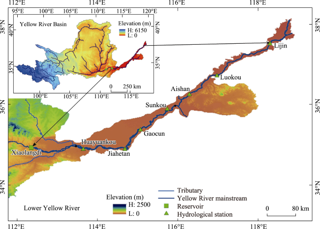
Figure 1 Sketch map of the Lower Yellow River
In this research, the input station is the Huayuankou station, and the measured water discharge, sediment concentration data, and coefficient of incoming sediment defined as the ratio of sediment concentration to corresponding water discharge from 2000 to 2020 were collected and organized, respectively. The output station is the Lijin station, and the water level at the discharge of 3000 m3/s at the Lijin station is taken as the erosion base level of the LYR. The erosion and deposition data are the annual measured accumulated deposition from the Huayuankou station to the Lijin station during the period of 2000-2020 (based on the deposition value in 1999), obtained by analysing the measured cross-sectional data of the LYR. The sediment particle size data in this research are based on the measured bed sediment particle size data from 7 hydrological stations in the LYR, represented by the median particle size D50 of the bed sediment.
The temporal variations of the coefficient of incoming sediment at the input station and the water level at the output station are shown in Figure 2. Figure 2a shows that there is a significant decrease in the annual average coefficient of incoming sediment at Huayuankou before and after the year 2000. After 2000, the coefficient of incoming sediment remained at a low level for a long time, with an annual average value fluctuating between 0.0005 and 0.0117 kg∙s/m6. The multiyear averaged value is 0.0045 kg·s/m6, which accounts for only 15.4% of the value in previous period (1986-1999).
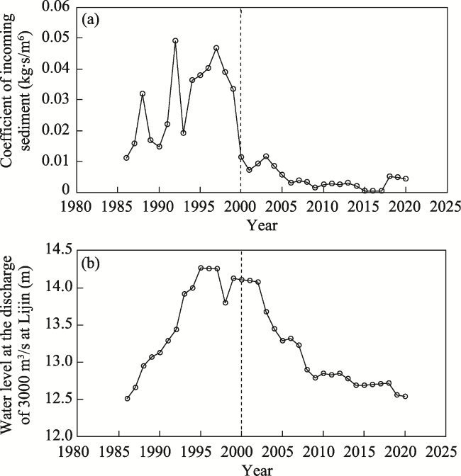
Figure 2 Inlet and outlet conditions of the Lower Yellow River: (a) Coefficient of incoming sediment at Huayuankou station, (b) Water level variation at Lijin station at the discharge of 3000 m3/s
With the operation of the Xiaolangdi Reservoir in 1999, the LYR gradually transformed from continuous deposition to continuous erosion, and the significant change in water and sediment conditions was one of the main reasons for the transition. From Figure 2b, it can be revealed that during the erosion period (2000-2020), the water level at the discharge of 3000 m3/s at Lijin station shows a decreasing trend over time, which is prone to form the headward erosion from downstream to upstream.

3 Derivation of the calculation formula for riverbed erosion and deposition

3.1 Derivation of the formula for the temporal variation of riverbed erosion and deposition

Due to the continuous variations in water and sediment conditions downstream of the Xiaolangdi Reservoir since its operation, it often happens that the adjustment of the riverbed has not fully dissolved the impact of water and sediment variations during a certain period, the next period's adjustment starts again, resulting in the riverbed being in a long-term and non-equilibrium continuous erosion process and gradually deviating from the original equilibrium state and empirical relationship. In addition, for the case of external disturbances with stepped changes, the adjustment results of the riverbed during one period, whether or not it has reached equilibrium, will serve as the initial conditions for the next period to affect the riverbed evolution and thus make the previous water and sediment conditions have an impact on the later riverbed evolution. The DRM proposed by Wu (2008a, 2008b) focuses on the temporal process and characteristics of riverbed evolution in a non-equilibrium state. Based on the single step mode of the DRM, the research period is divided into multiple subperiods ΔT, and the accumulated deposition at the end of the nth period can be represented as:
$V_{n}=\left(1-e^{-\beta_{n} \Delta T}\right) V_{e, n}+e^{-\beta_{n} \Delta T} V_{n-1} \quad(n \geqslant 1)$
where βn is the decay rate of riverbed erosion and deposition in the nth time period, and this parameter represents the adjustment rate. The larger the βn, the faster the adjustment of erosion and deposition; the smaller the βn, the slower the adjustment of erosion and deposition. Ve,n is the equilibrium value of accumulated deposition in the nth time period; Vn-1 is the accumulated deposition value at the end of the previous (n-1)th period.
Eq. (1) characterizes the temporal process of riverbed evolution in a non-equilibrium state. The equilibrium state is the target of the adjustment which is only a transient state in evolution process. The accurate simulation of the non-equilibrium evolution process of riverbed depends on the correct calculation of the equilibrium state of the riverbed, i.e., the equilibrium value of accumulated deposition, which needs to be determined based on specific issues. Generally, the variations in water level at the discharge of 3000 m3/s in the LYR can reflect the fluctuation of the riverbed caused by erosion and deposition. Figure 3 shows the longitudinal profile of the water level at the discharge of 3000 m3/s in the LYR in 2000 and 2015, respectively. As shown in Figure 3, the water level in the LYR decreases during the erosion period. Therefore, the longitudinal profile of the LYR when it reaches the erosion or deposition equilibrium state can be generalized as a trapezoidal deposition body, as shown in Figure 4. In Figure 4, J0 and Je represent the initial slope and equilibrium slope of the riverbed, respectively, and the shaded area in the figure represents the deposition body (Zheng, 2013). Δye1 and Δye2 are the thickness of the deposition body at the input station (Huayuankou) and the output station (Lijin), respectively. Assuming that the average width of the deposition body is B, based on the geometric relationship in Figure 4, the following formula for calculating the deposition volume in the equilibrium state can be obtained:
$V_{e}=\frac{B L}{2} \times\left(\Delta y_{e 1}+\Delta y_{e 2}\right)$
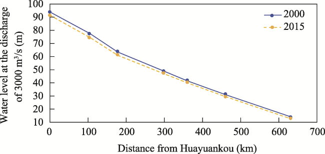
Figure 3 Comparison of water level at the discharge of 3000 m3/s in the Lower Yellow River
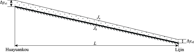
Figure 4 Schematic longitudinal profile of the Lower Yellow River
It is not difficult to find from the geometric relationship shown in Figure 4 that Δye1 and Δye2 have the following relationship:
$\Delta y_{e 1}=\Delta y_{e 2}+\left(J_{e}-J_{0}\right) \times L$
By substituting Eq. (3) into Eq. (2), the equilibrium value of accumulated deposition volume Ve can be calculated by:
$V_{e}=\frac{B L}{2} \times\left[\Delta y_{e 2}+\left(J_{e}-J_{0}\right) L+\Delta y_{e 2}\right]$
After simplification, Ve can be expressed as:
$V_{e}=\frac{B L^{2}}{2} \times\left(J_{e}-J_{0}\right)+B L \Delta y_{e 2}$
Based on previous research (Xie, 2013), the equilibrium slope of the riverbed Je can be expressed in the following form:
$J_{e}=k \bar{Q}^{a} \bar{S}^{b}$
where $\bar{Q}$ and $\bar{S}$ are the annual average water discharge and sediment concentration at the input station of the LYR, respectively. Meanwhile, considering that the riverbed slope is inversely proportional to the water discharge and directly proportional to the sediment concentration, the parameters k>0, a<0, b>0 in Eq. (6).
Considering the complex morphology of the river cross-section and the difficulty in accurately obtaining the riverbed elevation, the water level variation amount ΔZ at Lijin station corresponding to the discharge of 3000 m3/s is adopted to replace Δye2 in Eq. (5).
Substituting Eq. (6) and ΔZ into Eq. (5), the following calculation formula for the equilibrium deposition value Ve in the LYR can be obtained:
$V_{e}=\frac{B L^{2}}{2}\left(k \bar{Q}^{a} \bar{S}^{b}-J_{0}\right)+B L \Delta Z=K_{1} \bar{Q}^{a} \bar{S}^{b}+K_{2} \Delta Z+K_{3}$
where $K_{1}=\frac{k B L^{2}}{2}$, $K_{2}=B L$, and $K_{3}=-\frac{B L^{2}}{2} J_{0}$.
Eqs. (1) and (7) constitute the method for calculating the accumulated deposition in the LYR based on the DRM, which includes 6 parameters: K1, K2, K3, a, b, and β. The values of these parameters need to be calibrated based on the measured data. Considering the equilibrium slope coefficients k has the following relationship with K1 and K2:
$k=\frac{2 K_{1}}{L \times K_{2}}$
By substituting Eq. (8) into Eq. (6), Je can be expressed as:
$J_{e}=\frac{2 K_{1}}{L \times K_{2}} \bar{Q}^{a} \bar{S}^{b}$
Based on previous research (Wang et al., 2023), the variation range of the riverbed slope of the LYR is 1.00‱-1.90‱. Therefore, the reasonable variation range of the equilibrium slope Je represented by Eq. (9) is:
$1.00 ‱ \leqslant \frac{2 K_{1}}{L \times K_{2}} \bar{Q}^{a} \bar{S}^{b} \leqslant 1.90 ‱$
The initial slope of the riverbed J0 has the following relationship with K3 and K2:
$J_{0}=\frac{-2 K_{3}}{L \times K_{2}}$
Considering that J0 and Je should have essentially the same range of variation, it can be concluded that:
$1.00 ‱ \leqslant \frac{-2 K_{3}}{L \times K_{2}} \leqslant 1.90 ‱$

3.2 Derivation of the formula for the spatial variation of riverbed erosion and deposition

Sediment concentration in natural rivers is often in a non-equilibrium state, and it takes a process for suspended sediment concentration to reach equilibrium state through erosion and deposition. The non-equilibrium sediment transport equation considers the difference between sediment concentration and sediment transport capacity of water flow. The model generalizes the unsteady flow into steady flow, which means the water discharge Q is assumed to be constant in short-term calculation. Based on the non-equilibrium suspended sediment transport mechanism, the spatial variation of the cross-section average suspended sediment concentration in the non-uniform flow can be expressed as (Xie, 1990):
$\frac{d S}{d x}=-\alpha \frac{\omega}{q}\left(S-S_{*}\right)$
where S and S* represent the cross-section average suspended sediment concentration and sediment transport capacity, respectively, kg/m3; q is the unit width water discharge, m2/s; ω is the settling velocity of sediment particles, m/s; α is the saturation recovery coefficient of suspended sediment.
Assuming that the sediment transport capacity of the water flow varies linearly from upstream to downstream, then the formula for calculating the cross-section average suspended sediment concentration of non-uniform flow can be expressed as:
$S=S_{*}+\left(S_{0}-S_{0^{*}}\right) e^{-\frac{\alpha \omega l}{q}}+\left(S_{0^{*}}-S_{1^{*}}\right) \frac{q}{\alpha \omega L}\left(1-e^{-\frac{\alpha \omega l}{q}}\right)$
where subscript 0 represents the input station, and subscript 1 represents the output station; l is the length of the river reach (distance from the calculation section to the input station); L is the total length of the river.
By substituting Eq. (14) into Eq. (13), the formula for the spatial variation rate of sediment concentration can be obtained:
$\left.\frac{\mathrm{d} S}{\mathrm{~d} x}\right|_{l}=-\alpha \frac{\omega}{q}\left[\left(S_{0}-S_{0^{*}}\right) e^{-\frac{\alpha \omega l}{q}}+\left(S_{0^{*}}-S_{1^{*}}\right) \frac{q}{\alpha \omega L}\left(1-e^{-\frac{\alpha \omega l}{q}}\right)\right]$
Under the condition of constant water discharge, the spatial variation rate of erosion and deposition rate along the river can be expressed as:
$-\left.\frac{d Q_{s}}{d x}\right|_{l}=-\left.Q \frac{\mathrm{d} S}{\mathrm{~d} x}\right|_{l}$
where Q is the water discharge; Qs is the sediment transport rate of the river channel; x represents the distance from input station to the calculation section, from upstream to downstream.
By substituting Eq. (15) into Eq. (16), the spatial variation rate of erosion and deposition rate may be calculated by:
$-\left.\frac{d Q s}{d x}\right|_{l}=\alpha \omega B\left[\left(S_{0}-S_{0^{*}}\right) e^{-\frac{\alpha \omega l}{q}}+\left(S_{0^{*}}-S_{1^{*}}\right) \frac{q}{\alpha \omega L}\left(1-e^{-\frac{\alpha \omega l}{q}}\right)\right]$
By integrating Eq. (17) with time, the formula for the spatial distribution of accumulated erosion and deposition after time T can be obtained:
$V(l, T)=\int_{0}^{T} \alpha \omega B\left(S_{0}-S_{0^{*}}\right) e^{-\frac{\alpha \omega l}{q}}+\frac{\left(S_{0^{*}}-S_{1^{*}}\right) q B}{L}\left(1-e^{-\frac{\alpha \omega l}{q}}\right) d t$
By further simplifying Eq. (18), the following formula can be obtained for calculating the spatial variation of accumulated erosion and deposition per unit river length:
$V(l, T)=V_{a} \times e^{-\varphi l}+V_{b} \times\left(1-e^{-\varphi l}\right)$
where $V_{a}=\int_{0}^{T} \alpha \omega B\left(S_{0}-S_{0^{*}}\right) d t, V_{b}=\int_{0}^{T} \frac{\left(S_{0^{*}}-S_{1^{*}}\right) q B}{L} d t=\int_{0}^{T} \frac{\left(S_{0^{*}}-S_{1^{*}}\right) Q}{L} d t \cdot V_{a}$ is the erosion and deposition per unit river length at the input station, mainly caused by the difference between the sediment transport capacity and sediment concentration of the water flow at the input station. When the sediment concentration at the input station is greater than the corresponding sediment transport capacity of the water flow, Va>0; in contrast, when the sediment concentration at the input station is less than the corresponding sediment transport capacity of the water flow, Va<0. As erosion and deposition develop from upstream to downstream, the riverbed erosion and deposition caused by the difference in sediment transport capacity and sediment concentration at the input station will decrease gradually. Furthermore, when the distance from the input station is far enough, the weight of Va tends to disappear. Vb is caused by the spatial variation of sediment transport capacity, which may be defined as the spatial variation term of sediment transport capacity. If sediment transport capacity shows an increasing trend from upstream to downstream, then Vb <0. Whereas, if sediment transport capacity shows a decreasing trend, then Vb>0. Eq. (19) indicates that as the distance l increases, the value of erosion and deposition V will gradually approach Vb. Furthermore, when the distance is far enough, V will be approximately equal to Vb. $\varphi=\frac{\alpha \omega}{q}$, which is the spatial adjustment index of erosion and deposition, φ represents the rate at which the erosion and deposition adjusts from Va to Vb in space. The larger the φ, the faster the adjustment, and the smaller the φ, the slower the adjustment.

4 Simulation of the temporal adjustment process of riverbed erosion and deposition

Based on the measured erosion and deposition data of the LYR, the calculation method for accumulated deposition represented by Eqs. (1) and (7) is adopted to calibrate the parameters in the formula. The parameters taken to evaluate the accuracy of the calibration results are the coefficient of determination R2 and the relative error MNE. The corresponding calculation formulas are listed as follows:
$R^{2}=\frac{\left[\sum_{i=1}^{N}\left(y_{m, i}-\overline{y_{m}}\right)\left(y_{c, i}-\overline{y_{c}}\right)\right]^{2}}{\sum_{i=1}^{N}\left(y_{m, i}-\overline{y_{m}}\right)^{2} \sum_{i=1}^{N}\left(y_{c, i}-\overline{y_{c}}\right)^{2}}$
$M N E=\frac{1}{N} \sum_{i=1}^{N}\left|\frac{y_{c, i}-y_{m, i}}{y_{m, i}}\right| \times 100 \%$
where yc,i and ym,i represent the calculated and measured values of the characteristic variable y in the ith time period, respectively, while $\overline{y_{c}}$ and $\overline{y_{m}}$ represent the average calculated and measured values of the characteristic variable y over N time periods, respectively. R2 quantifies the degree of correlation between the calculated values and the measured values of the characteristic variable. The closer the value of R2 is to 1, the higher the correlation between the calculated values and the measured values; MNE quantifies the average relative error between the calculated values and the measured values of the characteristic variable. The closer the value of MNE is to 0, the higher the calculation accuracy.
After the operation of the Xiaolangdi Reservoir in 1999, the state of the riverbed of the LYR began to transform from deposition to erosion. The value of accumulated deposition and erosion base level in this research are based on the value in 1999 (set as 0 for both the accumulated deposition and the water level at the discharge of 3000 m3/s at Lijin station in 1999), and the calculation period is from 2000 to 2020. Based on the measured water and sediment data and accumulated deposition data from 2000 to 2020, taking ΔT=1 a as the time interval, the following formula for calculating the annual accumulated deposition in the LYR can be obtained through a nonlinear regression method:
$V_{n}=\left(1-e^{-0.23}\right)\left(237.7 \bar{Q}_{n}^{-0.053} \bar{S}_{n}^{0.01}+5 \Delta Z_{n}-175\right)+e^{-0.23} V_{n-1}$
where the decay rate β=0.23/a.
the formula of the equilibrium value of accumulated deposition is:
$V_{e, n}=237.7 \bar{Q}_{n}^{-0.053} \bar{S}_{n}^{0.01}+5 \Delta Z_{n}-175$
where $\bar{Q}_{n}$ and $\bar{S}_{n}$ are the annual average water discharge and sediment concentration at Huayuankou station in nth time period, and ΔZn is the accumulated variation value of the water level at Lijin station at the discharge of 3000 m3/s over n time periods.
The comparison between the calculated and measured values of accumulated deposition in the LYR from 2000 to 2020 is shown in Figure 5. The coefficient of determination between the calculated and measured values is equal to 0.99, and the average relative error is 16.5%, indicating high calculation accuracy of the DRM.
Figure 5 Comparison between calculated and measured values of accumulated deposition in the Lower Yellow River (Vm represents the measured value of accumulated deposition, and Vc represents the calculated value of accumulated deposition.)
Due to changes in incoming water and sediment conditions, as well as the downstream erosion base level, the equilibrium value of the accumulated deposition in the LYR has been constantly changing. Meanwhile, taking Ve as the target, the deposition volume V is adjusting constantly. In general, the relationship between the equilibrium value and the calculated value of accumulated deposition can be expressed as follows:
$V_{n-1}<V_{n}<V_{e, n} \quad \text { (in deposition) }$
$V_{n-1}>V_{n}>V_{e, n} \quad \text { (in erosion) }$
Figure 6a shows the relationship between the equilibrium value and the calculated value of accumulated deposition in the LYR, reflecting the delayed response characteristics between the accumulated deposition and the corresponding equilibrium or target value during each time period. Figure 6a reveals that the current equilibrium value of accumulated deposition from 2000 to 2020 is smaller than the calculated value at the end of the previous period. Therefore, during this period, the accumulated deposition adjusted in a decreasing direction, and the LYR experienced continuous erosion. After 2000, the erosion volume per unit runoff gradually decreased (Figure 7), indicating that with the continuous erosion, the riverbed gradually coarsened (Figure 12), and the erosion rate of the riverbed slowed down. Moreover, the difference between the equilibrium value of the current period and the calculated value at the end of previous period is decreasing in recent years, indicating that riverbed erosion is gradually approaching equilibrium (Figure 6a). Based on the Eq. (9), the temporal variations of the equilibrium slope of the generalized deposition body can be obtained (Figure 6b). From 2000 to 2020, with the continuous erosion in the LYR, the temporal variations of the equilibrium slope of the riverbed showed a decreasing trend, and the rate of decrease gradually slowed down. The decrease in the equilibrium slope is beneficial for slowing down the erosion rate. Meanwhile, with the coarsening of the riverbed (Miao et al., 2016), the adjustment of riverbed erosion is gradually approaching equilibrium, which reflects the equilibrium tendency of riverbed evolution. In addition, according to the derivation in section 3, K2=BL. Based on the value of K2 obtained from the calibration, the generalized river width is equal to 791 m, which is within the variation range of the bankfull width in the LYR (377-1226 m) (Wang et al., 2023).
Figure 6 The relationship between the equilibrium values and the calculated values of accumulated deposition in the Lower Yellow River (a) and the temporal variations of equilibrium slope of riverbed in the Lower Yellow River (b)
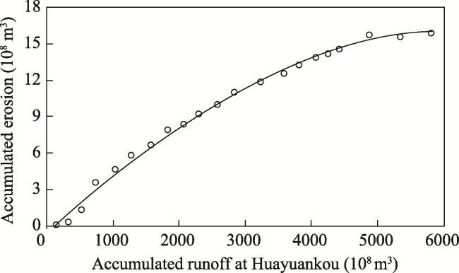
Figure 7 The relationship between accumulated runoff at HYK station and accumulated erosion in the Lower Yellow River
Based on the single step mode of the DRM and referring to the formula of adjustment time of the characteristic variable in previous research (Julien, 2018), the adjustment time of the accumulated deposition volume can be expressed as:
$t=-\frac{1}{\beta} \ln \left(\frac{V-V_{e}}{V_{0}-V_{e}}\right)$
where V is the adjustment value of the accumulated deposition, V0 is the initial value of the accumulated deposition, and Ve is the equilibrium value of the accumulated deposition.
The adjustment amount required for the accumulated deposition Vn to reach the equilibrium value Ve,n from the initial value Vn-1 is defined as the target adjustment amount ΔVn, which means ΔVn = Ve,n - Vn-1. The adjustment amount of erosion and deposition during the period is defined as the adjustment completion amount $\Delta V_{n}^{\prime}, \quad \Delta V_{n}^{\prime}=V_{n}-V_{n-1}$. Based on the DRM, the equilibrium value Ve,n can only be infinitely approached, which means Ve,n cannot be reached. To study the adjustment completion degree of erosion and deposition, the ratio of the adjustment completion amount $\Delta V_{n}^{\prime}$ to the target adjustment amount ΔVn is defined as completion degree m (the range of m is 0-1), and the time required to accomplish the completion degree is defined as the adjustment time Tm, where the erosion and deposition amount Vn = Vn-1 + m(Ve,n - Vn-1). Substituting the expression of Vn into Eq. (26), the calculation formula for adjustment time Tm can be obtained:
$T_{m}=-\frac{1}{\beta} \ln \left[\frac{V_{n-1}+m\left(V_{e, n}-V_{n-1}\right)-V_{e, n}}{V_{n-1}-V_{e, n}}\right]=-\frac{1}{\beta} \ln (1-m)$
Based on Eq. (27) and substituting in the value of decay rate β, the adjustment time T50, T60, T70, T80, T90, and T95 required for achieving adjustment ratio of 0.50 (half of the target adjustment amount), 0.60, 0.70, 0.80, 0.90, and 0.95 can be calculated, respectively. With the operation of the Xiaolangdi Reservoir in 1999, the sediment load entering the LYR has sharply decreased, leading to long-term and continuous erosion. Based on the calculation results in section 4, the decay rate β=0.23/a. By substituting β into Eq. (27), the time required for the adjustment of deposition to reach different completion degree can be calculated (Table 1). For example, in the background of decreasing sediment inflow and river channel erosion, for the initial riverbed of any year, under the conditions of constant upstream water and sediment conditions and downstream erosion base level, the time required to accomplish half of the accumulated deposition adjustment is approximately 3.0 years, and the time required to reach a quasi-equilibrium state (95% of the accumulated deposition adjustment to be completed) is approximately 13.0 years.
Table 1 The time required for the adjustment of accumulated deposition to accomplish different adjustment degrees
m 0.5 0.6 0.7 0.8 0.9 0.95
Tm /a 3.0 4.0 5.2 7.0 10.0 13.0

5 Simulation of the spatial variation process of riverbed erosion and deposition

The spatial distribution characteristics of riverbed erosion and deposition in the LYR are the result of the coupling effect of downward and headward erosion and deposition. The spatial distribution of accumulated main channel erosion and deposition per unit river length in the LYR from 2003 to 2015 can be simulated based on Eq. (19). The calibration results of the key parameters such as the erosion and deposition at the input station Va, the sediment transport capacity variation term Vb, and the spatial adjustment index φ are shown in Table 2, and the comparison between calculated and the measured values of accumulated main channel erosion and deposition per unit river length is shown in Figure 8 (the figure only lists the results of odd years).
Table 2 Key parameters for the simulation of erosion and deposition volume in the Lower Yellow River during erosion period
Va (104 m3/m) φ Vb (104 m3/m) R2 MNE (%)
2003 -0.4502 0.0183 -0.0194 0.9962 12.3
2004 -0.4347 0.0141 -0.029 0.9856 17.9
2005 -0.4753 0.0128 -0.0423 0.9807 15.5
2006 -0.6091 0.0132 -0.0427 0.9974 7.0
2007 -0.6704 0.0128 -0.054 0.9994 2.7
2008 -0.6772 0.0121 -0.0563 0.9993 3.4
2009 -0.6913 0.011 -0.0587 0.9991 4.0
2010 -0.7306 0.0109 -0.0653 0.9996 2.4
2011 -0.7684 0.0099 -0.0664 0.9997 2.4
2012 -0.8294 0.0098 -0.0722 0.9997 1.9
2013 -0.866 0.0097 -0.078 0.9992 2.7
2014 -0.9186 0.0095 -0.0772 0.9988 4.6
2015 -0.977 0.0093 -0.0747 0.9993 3.6
Figure 8 Comparison between calculated and measured values of accumulated erosion and deposition volume per unit river length in the main channel of the Lower Yellow River
From Table 2 and Figure 8, it can be concluded that Eq. (19) can effectively simulate the spatial distribution of accumulated main channel erosion and deposition per unit river length in the LYR. The coefficient of determination R2 between the fitted values and the measured values is higher than 0.98, and the relative error is lower than 18%. Table 2 reveals that the absolute value of Va during the erosion period increased over time. Considering that the coefficient of incoming sediment shows a decreasing trend since 2000 and has remained at an extremely low level for a long time, the main reason for the temporal increase in the absolute value of Va may be the water flow at the input station has been in an unsaturated state and needs to scour the riverbed to supplement sediment. It can be foreseen that if the current water and sediment conditions at the input station are maintained in the future, the absolute value of Va will continue to increase. However, due to the coarsening of riverbed sediment, which means the increase in resistance to water flow, the increase rate of Va may slow down.
Note that the erosion amount in the LYR tends to approach the spatial equilibrium value Vb near the lower part of the river, rather than approaching 0, and the absolute value of the spatial equilibrium value Vb shows an increasing trend over time. It can be concluded that the sediment transport capacity of the water flow in the LYR has a spatial enhancement trend to some extent, which may be due to factors such as narrowing of the cross-section, fining of bed sediment, and decrease in erosion base level. The combined effect of these factors induces that the water flow still has erosion ability near the output station of the LYR, enabling the continuous development of riverbed erosion along the river.
Figure 9 shows the spatial variations of sediment concentration and coefficient of incoming sediment along the LYR. From Figure 9, it can be concluded that the sediment concentration has an approximately linear increasing trend in space, whereas the coefficient of incoming sediment shows an exponential increasing trend along the river. Based on Eq. (13), combined with the calibration results in Table 2 and Figure 8, it can be concluded that the sediment transport capacity of the water flow in the LYR is generally higher than the sediment concentration after the operation of the Xiaolangdi Reservoir. Therefore, a widespread and continuous erosion exists from upstream to downstream, and the water flow supplements sediment through erosion along the way, causing the sediment concentration to show an increasing pattern from upstream to downstream. This is a typical case of the spatial adjustment of sediment-laden flow from non-equilibrium to equilibrium.
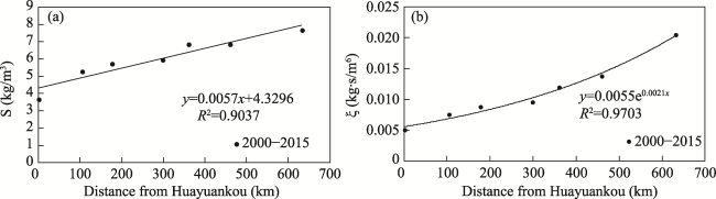
Figure 9 Spatial variations of sediment concentration (a) and coefficient of incoming sediment (b) in the Lower Yellow River during the period 2000-2015
The Shields number reflects the relative magnitude of the shear stress exerted on sediment particles by water flow and the resistance force exerted on sediment particles. The larger the Shields number, the more easily the bed sediment is washed away by water flow. The calculation formula is:
$\theta=\frac{\gamma h J}{\left(\gamma_{s}-\gamma\right) D}$
where γ is the unit weight of clear water; γs is the unit weight of sediment particles; J is the slope of the river, which can be approximately replaced by the riverbed slope; and D is the particle size of bed sediment; h is the average water depth of main channel before and after flood season.
The changes in the unit weight of clear water and sediment particles are not significant, therefore these two parameters can be approximately treated as constants. Taking the median particle size of the bed sediment D50 as the representative particle size, then Eq. (28) can be simplified as the following flow intensity parameter (Wu and Zheng, 2015):
$\sigma=\frac{h J}{\bar{D}_{50}}$
where h is the average water depth in the main channel of the LYR before and after the flood season, obtained based on measured cross-sectional data of each reach in the LYR; J is the riverbed slope of the LYR, obtained by referring to relevant research (Wang et al., 2023); $\bar{D}_{50}$ is the average median bed sediment particle size in each river reach, for example, the average median particle size of riverbed sediment of the Hua-Jia reach is the average value of median particle size of riverbed sediment at Huayuankou station and Jiahetan station.
The flow intensity parameter σ can reflect the erosion capacity of water flow, and the calculation results are shown in Figure 10. According to Figure 10, it can be concluded that, in general, during the continuous erosion period after 2000, the flow's erosion capacity towards the riverbed increased from upstream to downstream in the LYR, which may be one of the reasons why the water flow of the LYR still has a certain erosion capacity when approaching the output station.
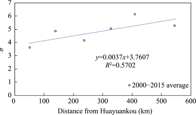
Figure 10 Spatial distribution of flow intensity parameter σ in the Lower Yellow River
The temporal variations of spatial adjustment index of erosion and deposition φ is shown in Figure 11a. In general, the value of φ shows a decreasing trend over time. This decreasing trend indicates that the adjustment of the accumulated erosion and deposition per unit river length from the value at the input station Va to the spatial variation term of sediment transport capacity Vb gradually slows down. To analyse the uniformity of the spatial distribution of erosion in the LYR, this research proposed the parameter L0.5. The midpoint of erosion L0.5 is defined as the position where the accumulated erosion originating from Huayuankou (input station) reaches half of the total erosion in the LYR. The smaller the L0.5, the more concentrated the riverbed erosion distributed in the upper part of the river, and the more nonuniform the spatial distribution of riverbed erosion, whereas the larger the L0.5, the more uniform the spatial distribution of riverbed erosion. Based on the values of Va, Vb, and φ listed in Table 2, it is not difficult to obtain the annual calculated value of L0.5 through integration, and the calculation result of L0.5 is shown in Figure 11b.
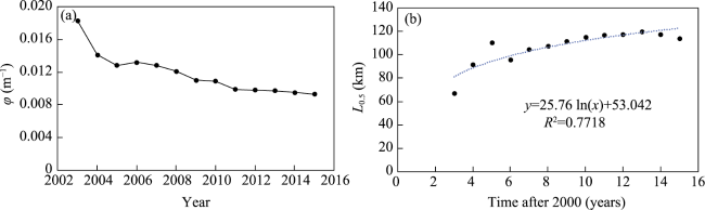
Figure 11 Temporal variations of spatial adjustment index of erosion (a) and midpoint of erosion in the Lower Yellow River (b)
The year 2000 when erosion began in the LYR is defined as the initial year. As shown in Figure 11b, L0.5 shows an overall increasing trend over time, indicating that with the continuous development of riverbed erosion, the spatial distribution of accumulated erosion in the LYR will gradually become uniform. When there is less sediment and more water entering the LYR, the riverbed undergoes erosion from upstream to downstream, and the sediment concentration in the water gradually recovers from upstream to downstream. Compared with the lower part of the LYR, the upper part of the LYR has a greater degree of sediment unsaturation, therefore the erosion capacity of water flow on the riverbed is more significant, forming a decreasing spatial pattern of accumulated erosion in recent years.
Corresponding to the spatial pattern of accumulated erosion, the riverbed composition exhibits a severe coarsening phenomenon (Figure 12a), and the median particle sizes of bed sediment also shows a decreasing trend from upstream to downstream (Figure 12b). In addition, the upper part of the LYR has a relatively larger amount of erosion, therefore, its riverbed slope has a decreasing trend with the continuous development of erosion. Under the joint effect of the above factors, when erosion develops to a certain degree, the boundary conditions of the lower part of the LYR are more prone to be eroded than those of the upper part of the river. Therefore, in recent years, when the accumulated erosion per unit river length maintained a decreasing pattern from upstream to downstream in the LYR, the difference in erosion amounts between the upper and lower parts of the LYR decreased gradually. This process reflects the equilibrium tendency of riverbed evolution.
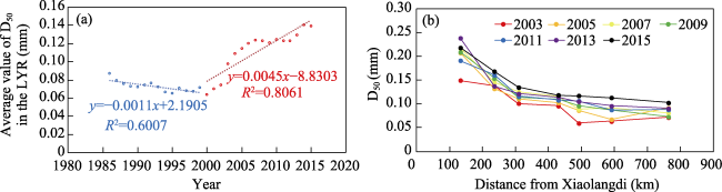
Figure 12 Temporal and spatial variations of median particle size of bed sediment in the Lower Yellow River

6 Conclusions

(1) Based on the DRM and the generalized equilibrium geometry of the deposition body, the method for calculating the accumulated deposition in the LYR has been established. The coefficient of determination R2 between the calculated and measured values from 2000 to 2020 reached 0.99, indicating good calculation results. With the continuous erosion of the riverbed by water flow, the erosion rate of the riverbed in the LYR shows a decreasing trend.
(2) Based on the non-equilibrium sediment transport equation, the formula for calculating the spatial distribution of accumulated main channel erosion and deposition per unit river length has been derived. The formula can effectively simulate the spatial distribution characteristics of erosion and deposition amount in the LYR. The coefficient of determination R2 between the fitted values and the measured values from 2003 to 2015 is between 0.98 and 0.99, with an average relative error of 6.2% for the research period.
(3) Since the operation of Xiaolangdi Reservoir, the equilibrium riverbed slope of the LYR has been decreasing over time, and the rate of decrease has gradually slowed down. For the initial riverbed of any year, if the upstream water and sediment conditions and the downstream erosion base level remain constant, the time required to complete half of the accumulated deposition adjustment is approximately 3.0 years, and the time required to complete 95% of the adjustment is approximately 13.0 years.
[1]
An C, Fu X, 2022. Theory of delayed response in river morphodynamics: Applicability and limitations. International Journal of Sediment Research, 37 (2): 162-172.

DOI

[2]
An C H, Lu J, Wu M X et al., 2020. The threshold value of equilibrium sediment transport in the Lower Yellow River. Journal of Hydraulic Engineering, 51(4): 402-409. (in Chinese)

[3]
Graf W L, 1977. The rate law in fluvial geomorphology. American Journal of Science, 277(2): 178-191.

DOI

[4]
Jing H, Zhong D Y, Zhang H W et al., 2020. The accumulation phenomenon and stochastic model in fluvial processes. Acta Geographica Sinica, 75(5): 1079-1094. (in Chinese)

DOI

[5]
Julien P Y, 2018. River Mechanics. Cambridge: Cambridge University Press.

[6]
Knighton D, 1998. Fluvial Forms and Processes:A New Perspective. New York: Wiley.

[7]
Li Q, Lu Z C, 1989. Mathematical approach to the effect of change of river caused by the longitudinal and upstream deposition in the lower reaches of the Huanghe River. Scientia Geographica Sinica, 9(4): 336-345. (in Chinese)

DOI

[8]
Liu S W, Wang Z L, Li D X, 2022. Comparison of sediment carrying capacity to sediment concentration in the upper reaches of the Yangtze River. Journal of Hydroelectric Engineering, 41(11): 10. (in Chinese)

[9]
Long Y Q, 2002. Range survey of deposition in the lower Yellow River. International Journal of Sediment Research, (2): 91-101.

[10]
Lu Z C, Zhou J X, Chen H, 2003. River bed longitudinal profile morphology of the Lower Yellow River and its implication in physiography. Geographical Research, 22(1): 30-38. (in Chinese)

DOI

[11]
Lyu Y W, Zheng S, Tan G M et al., 2019. Morphodynamic adjustments in the Yichang-Chenglingji reach of the Middle Yangtze River since the operation of the Three Gorges Project. Catena, 172: 274-284.

DOI

[12]
Miao C Y, Kong D X, Wu J W et al., 2016. Functional degradation of the water-sediment regulation scheme in the lower Yellow River: Spatial and temporal analyse. Science of the Total Environment, 551/552(May): 16-22.

[13]
Qian N, Zhang R, Zhou Z D, 1987. Fluvial Processes. Beijing: Science Press. (in Chinese)

[14]
Qian N, Zhou W H, 1965. Fluvial Processes in the Lower Yellow River. Beijing: Science Press. (in Chinese)

[15]
Simon A, Rinaldi M, 2006. Disturbance, stream incision, and channel evolution: The roles of excess transport capacity and boundary materials in controlling channel response. Geomorphology, 79(3/4): 361-383.

DOI

[16]
Surian N, Rinaldi M, 2003. Morphological response to river engineering and management in alluvial channels in Italy. Geomorphology, 50(4): 307-326.

DOI

[17]
Wang Y J, Wu B S, Zhong D Y et al., 2016. Calculation method for sediment load in flood and non-flood seasons in the Inner Mongolia reach of the Yellow River. Journal of Geographical Sciences, 26(6): 707-721.

DOI

[18]
Wang Y J, Wu B S, Zhong D Y, 2020a. Adjustment in the main-channel geometry of the lower Yellow River before and after the operation of the Xiaolangdi Reservoir from 1986 to 2015. Journal of Geographical Sciences, 30(3): 468-486.

DOI

[19]
Wang Y J, Wu B S, Zhong D Y, 2020b. Simulating cross-sectional geometry of the main channel in response to changes in water and sediment in Lower Yellow River. Journal of Geographical Sciences, 30(12): 2033-2052.

DOI

[20]
Wang Y Z, Xia J Q, Deng S S et al., 2023. Coupled modelling of bank erosion and accretion in the Lower Yellow River. Advanced Engineering Sciences, 55(4): 130-141. (in Chinese)

[21]
Wu B S, 2008a. Delayed response model for fluvial processes of alluvial rivers (I): Model development. Journal of Sediment Research, (6): 1-7. (in Chinese)

[22]
Wu B S, 2008b. Delayed response model for fluvial processes of alluvial rivers (Ⅱ): Model applications. Journal of Sediment Research, (6): 30-37. (in Chinese)

[23]
Wu B S, Wang G Q, Xia J Q, 2007. Case study: Delayed sedimentation responses to inflow and operations at Sanmenxia Dam. Journal of Hydraulic Engineering, 133(5): 482-494.

DOI

[24]
Wu B S, Wang G Q, Xia J Q et al., 2008. Response of bankfull discharge to discharge and sediment load in the Lower Yellow River. Geomorphology, 100(3/4): 366-376.

DOI

[25]
Wu B S, Xia J Q, Wang Z Y, 2006. Delayed response of Tongguan's elevation to the sedimentation in Sanmenxia Reservoir. Journal of Sediment Research, (1): 8-16. (in Chinese)

[26]
Wu B S, Zheng S, 2015. Delayed Response Theory and Applications for Fluvial Processes. Beijing: China Water&Power Press. (in Chinese)

[27]
Wu B S, Zheng S, Thorne C R, 2012. A general framework for using the rate law to simulate morphological response to disturbance in the fluvial system. Progress in Physical Geography, 36(5): 575-597.

[28]
Xia J Q, Deng S S, Lu J Y et al., 2016. Dynamic channel adjustments in the Jingjiang reach of the Middle Yangtze River. Scientific Reports, 6: 22802.

DOI PMID

[29]
Xia J Q, Li X J, Li T et al., 2014. Response of reach-scale bankfull channel geometry to the altered flow and sediment regime in the lower Yellow River. Geomorphology, 213(May 15): 255-265.

DOI

[30]
Xia J Q, Wu B S, Wang Y P, 2008. Processes and characteristics of recent channel adjustment in the Lower Yellow River. Advances in Water Science, (3): 301-308. (in Chinese)

[31]
Xie J H, 1990. River Simulation. Beijing: Water Conservancy and Electric Power Press. (in Chinese)

[32]
Xie J H, 2013. Riverbed Evolution and Renovation. Wuhan: Wuhan University Press. (in Chinese)

[33]
Zhang R Y, Wang Y J, Han Q L et al., 2018. Calculation methods for erosion and deposition based on sediment balance equation in the Lower Yellow River. Journal of Sediment Research, 43(3): 21-28. (in Chinese)

[34]
Zhang X F, Liu X N, Wu B S, 2010. Fluvial Dynamics. Beijing: China Water Resources and Hydropower Press. (in Chinese)

[35]
Zheng S, 2013. Study on the simulation of non-equilibrium fluvial processes[D]. Beijing: Tsinghua University. (in Chinese)

[36]
Zheng S, Wu B S, Thorne C R et al., 2015. Case study of variation of sedimentation in the Yellow and Wei rivers. Journal of Hydraulic Engineering, 141(3): 05014009. 1-05014009.10.

Outlines

/