
Journal of Geographical Sciences >
Quantitative response of vegetation phenology to temperature and precipitation changes in Eastern Siberia
|
We Kege (1987-), PhD, specialized in applications of remote sensing of resources and environment and geographic information system. E-mail: Wenkege@mail.cgs.gov.cn |
Received date: 2023-06-13
Accepted date: 2023-10-17
Online published: 2024-02-06
Supported by
International Cooperation and Exchange of the National Natural Science Foundation of China(42061134019)
Major Special Project-The China High-Resolution Earth Observation System(30-Y30F06-9003-20/22)
Significant changes to the world’s climate over the past few decades have had an impact on the development of plants. Vegetation in high latitude regions, where the ecosystems are fragile, is susceptible to climate change. It is possible to better understand vegetation’s phenological response to climate change by examining these areas. Traditional studies have mainly investigated how a single meteorological factor affects changes in vegetation phenology through linear correlation analysis, which is insufficient for quantitatively revealing the effects of various climate factor interactions on changes in vegetation phenology. We used the asymmetric Gaussian method to fit the normalized difference vegetation index (NDVI) curve and then used the dynamic threshold method to extract the phenological parameters, including the start of the season (SOS), end of the season (EOS), and length of the season (LOS), of the vegetation in this study area in the Tundra-Tagar transitional zone in eastern and western Siberia from 2000 to 2017. The monthly temperature and precipitation data used in this study were obtained from the climate research unit (CRU) meteorological dataset. The degrees to which the changes in temperature and precipitation in the various months and their interactions affected the changes in the three phenological parameters were determined using the GeoDetector, and the results were explicable. The findings demonstrate that the EOS was more susceptible to climate change than the SOS. The vegetation phenology shift was best explained by the climate in March, April, and September, and the combined effect of the temperature and precipitation had a greater impact on the change in the vegetation phenology compared with the effects of the individual climate conditions. The results quantitatively show the degree of interaction between the variations in temperature and precipitation and their effects on the changes in the different phenological parameters in the various months. Understanding how various climatic variations effect phenology changes in plants at different times may be more intuitive. This research provides as a foundation for research on how global climate change affects ecosystems and the global carbon cycle.
Key words: phenology; climate change; Siberia; asymmetric Gaussian function; GeoDetector
WEN Kege , LI Cheng , HE Jianfeng , ZHUANG Dafang . Quantitative response of vegetation phenology to temperature and precipitation changes in Eastern Siberia[J]. Journal of Geographical Sciences, 2024 , 34(2) : 355 -374 . DOI: 10.1007/s11442-024-2208-0
Figure 1 Study area shown in the world map and NDVI of study area (a); landcover map of the study area (b) |
Table 1 Definition of vegetation growth season parameters |
| Vegetation growth season parameter | Definition |
|---|---|
| SOS | When the left edge, as measured from the left minimum level, has risen to 10%. |
| EOS | When the right edge, as measured from the right minimum level, has shrunk to 10%. |
| LOS | Duration of the season, from the beginning to the end. |
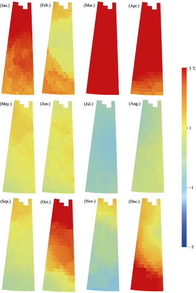
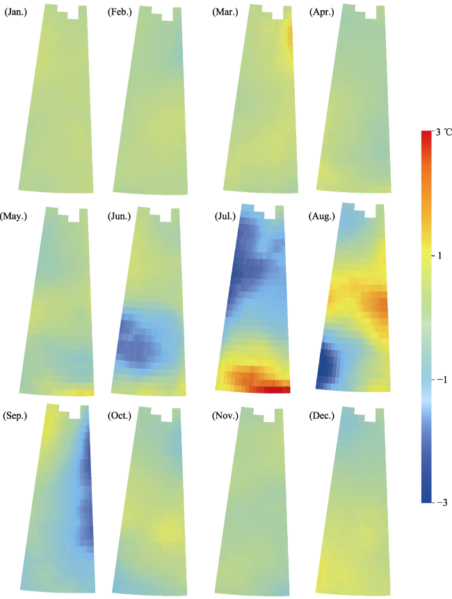
Figure 2 Linear trend of monthly mean temperature in the study area from 2000 to 2017 |
Figure 3 Linear trend of monthly precipitation in the study area from 2000 to 2017 |
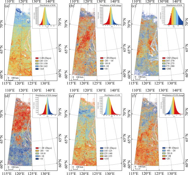
Figure 4 Spatial distribution of the mean SOS (a), EOS (c), and LOS (e) for the 18-year period between 2000 and 2017 and the linear regression-based difference in SOS (b), EOS (d), and LOS (f) in the same period |
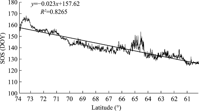
Figure 5 SOS distribution trend along latitude |
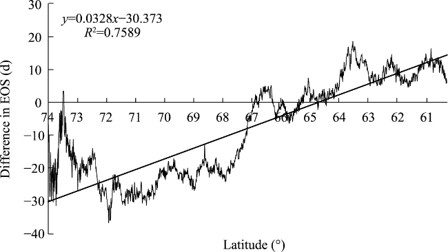
Figure 6 Difference in EOS distribution trend along latitude |
Table 2 Qs and the significance of phenological parameters trends interpreted by monthly mean temperature |
| SOS | EOS | LOS | ||||
|---|---|---|---|---|---|---|
| Q | pValue | Q | pValue | Q | pValue | |
| T1 | 0.074 | 0.000 | 0.341* | 0.000 | 0.274* | 0.000 |
| T2 | 0.086 | 0.000 | 0.273* | 0.000 | 0.198 | 0.000 |
| T3 | 0.049 | 0.000 | 0.371* | 0.000 | 0.241* | 0.000 |
| T4 | 0.079 | 0.000 | 0.384* | 0.000 | 0.275* | 0.000 |
| T5 | 0.016 | 0.606 | 0.332* | 0.000 | 0.227* | 0.000 |
| T6 | 0.036 | 0.000 | 0.157 | 0.000 | 0.101 | 0.000 |
| T7 | 0.052 | 0.000 | 0.128 | 0.000 | 0.061 | 0.000 |
| T8 | 0.069 | 0.000 | 0.283* | 0.000 | 0.231* | 0.000 |
| T9 | 0.105 | 0.000 | 0.375* | 0.000 | 0.289* | 0.000 |
| T10 | 0.062 | 0.000 | 0.307* | 0.000 | 0.246* | 0.000 |
| T11 | 0.072 | 0.000 | 0.332* | 0.000 | 0.243* | 0.000 |
| T12 | 0.028 | 0.007 | 0.297* | 0.000 | 0.203* | 0.000 |
| P1 | 0.020 | 0.173 | 0.157 | 0.000 | 0.123 | 0.000 |
| P2 | 0.053 | 0.000 | 0.260* | 0.000 | 0.238* | 0.000 |
| P3 | 0.046 | 0.000 | 0.101 | 0.000 | 0.075 | 0.000 |
| P4 | 0.073 | 0.000 | 0.181 | 0.000 | 0.176 | 0.000 |
| P5 | 0.048 | 0.000 | 0.080 | 0.000 | 0.071 | 0.000 |
| P6 | 0.046 | 0.000 | 0.222* | 0.000 | 0.174 | 0.000 |
| P7 | 0.036 | 0.000 | 0.321* | 0.000 | 0.182 | 0.000 |
| P8 | 0.069 | 0.000 | 0.136 | 0.000 | 0.108 | 0.000 |
| P9 | 0.036 | 0.000 | 0.100 | 0.000 | 0.106 | 0.000 |
| P10 | 0.055 | 0.000 | 0.052 | 0.000 | 0.054 | 0.000 |
| P11 | 0.053 | 0.000 | 0.111 | 0.000 | 0.102 | 0.000 |
| P12 | 0.079 | 0.000 | 0.353* | 0.000 | 0.269* | 0.000 |
Table 3 Qs of sOs trends interpreted by interaction of temperature and precipitation |
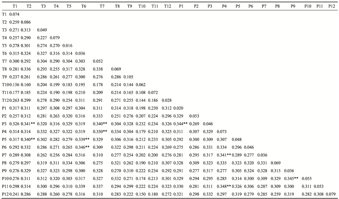 |
Note: **Top ten in terms of interpretations. |
Table 4 Qs of EOS trends interpreted by interaction of temperature and precipitation |
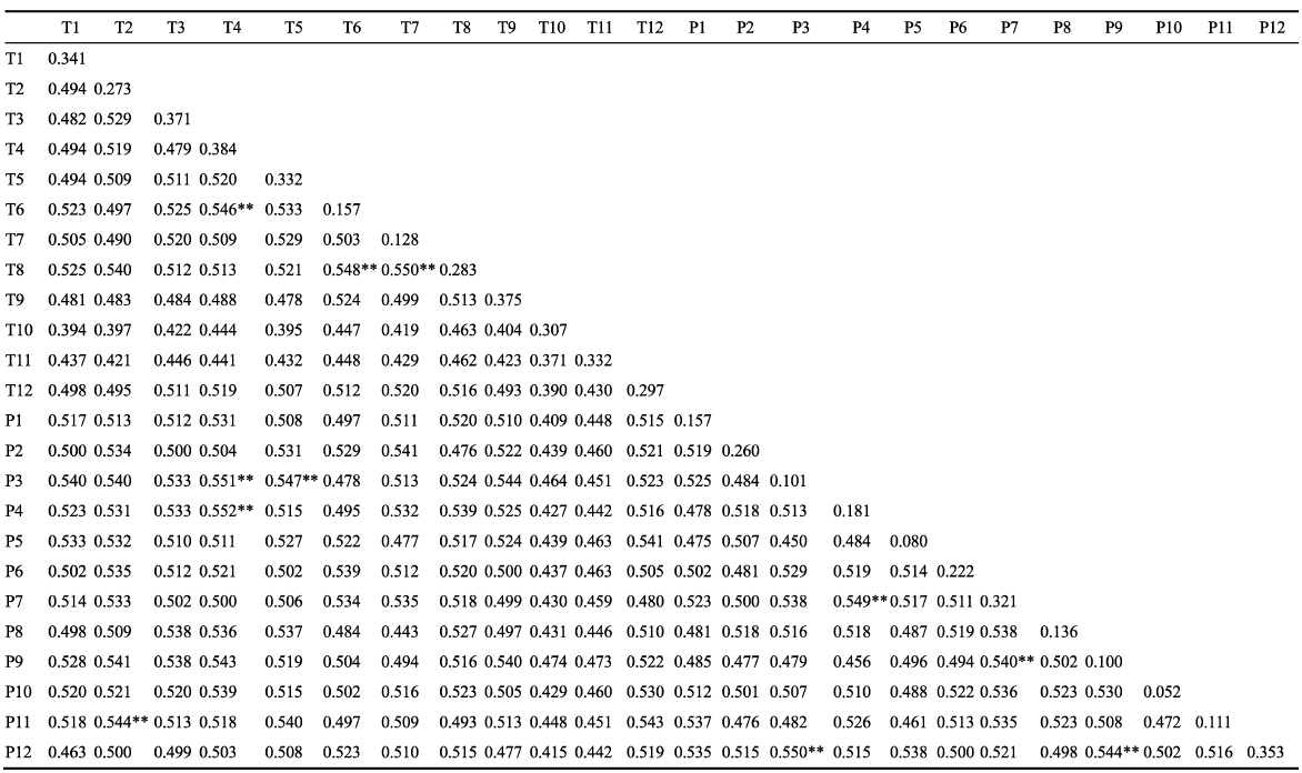 |
Note: **Top ten in terms of interpretations. |
Table 5 Qs of LOS trends interpreted by interaction of temperature and precipitation |
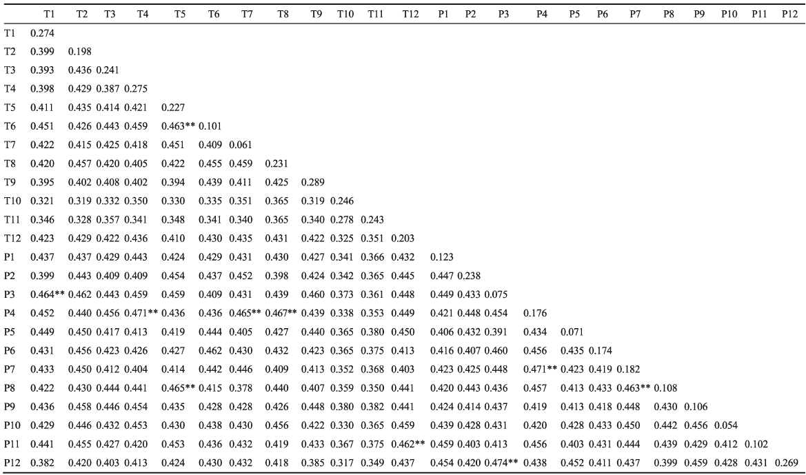 |
Note: **Top ten in terms of interpretations. |
| [1] |
|
| [2] |
|
| [3] |
|
| [4] |
|
| [5] |
|
| [6] |
|
| [7] |
|
| [8] |
|
| [9] |
|
| [10] |
|
| [11] |
|
| [12] |
|
| [13] |
|
| [14] |
|
| [15] |
|
| [16] |
|
| [17] |
|
| [18] |
|
| [19] |
|
| [20] |
|
| [21] |
|
| [22] |
|
| [23] |
|
| [24] |
|
| [25] |
|
| [26] |
|
| [27] |
|
| [28] |
|
| [29] |
|
| [30] |
|
| [31] |
|
/
| 〈 |
|
〉 |
