
Journal of Geographical Sciences >
Evaluating flash flood simulation capability with respect to rainfall temporal variability in a small mountainous catchment
|
Wang Xuemei (1998-), PhD Candidate, specialized in hydrology and water resources. E-mail: wang_xmww@163.com |
Received date: 2022-12-27
Accepted date: 2023-09-26
Online published: 2023-12-14
Supported by
National Natural Science Foundation of China(42171047)
National Natural Science Foundation of China(42071041)
Rainfall temporal patterns significantly affect variability of flash flood behaviors, and further act on hydrological model performances in operational flash flood forecasting and warning. In this study, multivariate statistical analysis and hydrological simulations (XAJ and CNFF models) were combined to identify typical rainfall temporal patterns and evaluate model simulation capability for water balances, hydrographs, and flash flood behaviors under various rainfall patterns. Results showed that all the rainfall events were clustered into three types (Type 1, Type 2, and Type 3) in Anhe catchment in southeastern China. Type 1 was characterized by small total amount, high intensity, short duration, early peak moment, and concentrated hourly distribution. Type 3 was characterized by great total amount, low intensity, long duration, late peak moment, and uniform hourly distribution. Characteristics of Type 2 laid between those of Type 1 and Type 3. XAJ and CNFF better simulated water balances and hydrographs for Type 3, as well as all flash flood behavior indices and flood dynamics indices. Flood peak indices were competitively simulated for all the types by XAJ and except Type 1 by CNFF. The study is of significance for understanding relationships between rainfall and flash flood behaviors and accurately evaluating flash flood simulations.
WANG Xuemei , ZHAI Xiaoyan , ZHANG Yongyong , GUO Liang . Evaluating flash flood simulation capability with respect to rainfall temporal variability in a small mountainous catchment[J]. Journal of Geographical Sciences, 2023 , 33(12) : 2530 -2548 . DOI: 10.1007/s11442-023-2188-5
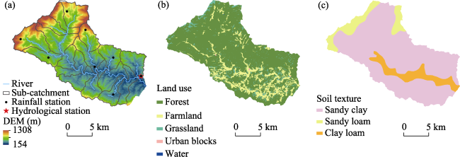
Figure 1 Spatial distribution of DEM and water system (a), land use (b) and soil texture types (c) in Anhe catchment |
Table 1 Selected rainfall characteristic indices at event scale |
| Category | Index | Abbreviation | Unit | Equation |
|---|---|---|---|---|
| Magnitude | Total rainfall amount | P | mm | $P=\sum\limits_{t={{F}_{begin}}}^{{{F}_{end}}}{{{p}_{t}}}$ |
| Average rainfall amount | AP | mm | AP=P/T | |
| Intensity | Maximum rainfall intensity | MPI | mm/h | MPI = max(Pt) |
| Time | Rainfall duration | T | h | $T={{F}_{end}}-{{F}_{begin}}+1$ |
| Peak rainfall moment coefficient | ${{R}_{MPI}}$ | - | ${{R}_{MPI}}={{{F}_{MP}}_{I}}/{T}\;$ | |
| Concentration | Rainfall concentration | PCI | - | PCI=MPI/P |
Notes: pt is the rainfall amount at time t, mm; Fbegin and Fend are the time when a rainfall event begins and ends, respectively, h; FMPI is the occurrence time of the maximum rainfall intensity, h. |
Table 2 Selected flash flood behavior indices at event scale |
| Category | Index | Abbreviation | Unit | Equation |
|---|---|---|---|---|
| Peak | Peak flow modulus | Km | m3/(s·km2) | Km=Qm/A |
| Peak flow occurrence time | Tm | h | Tm=T(Qm) | |
| Lag time | Tl | h | Tl=Tm-FMPI | |
| Dynamics | Average rate of rising limb | RQ | s-1 | $RQ=\frac{3600\left( {{Q}_{m}}-{{Q}_{begin}} \right)}{\left( Tm-{{T}_{begin}} \right)\sum\limits_{t={{T}_{begin}}}^{{{T}_{end}}}{{{Q}_{t}}}}$ |
| Average rate of declining limb | DQ | s-1 | $DQ=\frac{3600\left( {{Q}_{m}}-{{Q}_{end}} \right)}{\left( {{T}_{end}}-Tm \right)\sum\limits_{t={{T}_{begin}}}^{{{T}_{end}}}{{{Q}_{t}}}}$ | |
| Flood hydrograph kurtosis | K | - | $K=\frac{1}{N}\sum\limits_{t={{T}_{begin}}}^{{{T}_{end}}}{{{\left( \frac{{{Q}_{t}}-\mu }{\sigma } \right)}^{4}}}$ |
Notes: Qm is the peak flow, m3/s; A is the catchment area, km2; Qbegin, Qend and Qt are the flood flows at time Tbegin, Tend and t, respectively, m3/s; Tbegin and Tend are the time when a flood process begins and ends, respectively, h; μ and σ are the average value and standard deviation value of a flood process, respectively. |
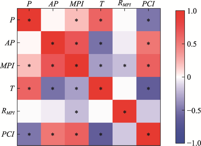
Figure 2 Correlation coefficients of rainfall characteristic indicesNote: * indicates the correlation coefficient has a significance level p<0.05. |
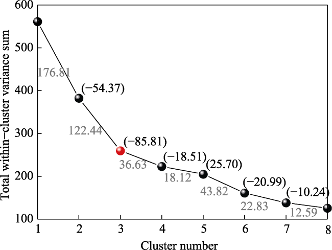
Figure 3 The diagram of total within-cluster variance sum (Vartotal) versus cluster number (K)Notes: The number on the broken line between K=i and K=i+1 (1≤i≤7) represents the decreasing rate of Vartotal with K increasing from i to i+1, which is noted as Vartotal(i)*. The number within the bracket represents the difference between Vartotal(i+1)* and Vartotal(i)*, which is noted as Vartotal(i+1)#. The red point represents the optimal cluster number K, which is the elbow inflection point of the curve with the minimum Vartotal(K=3)#. |
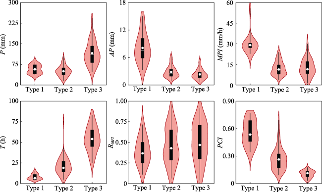
Figure 4 Distribution of rainfall characteristic indices for three rainfall typesNotes: Boxes represent the ranges from the 25th to the 75th quartiles, whiskers represent the ranges from the minimum to the maximum, and dots and lines in boxes represent the averages and the medians, respectively. |
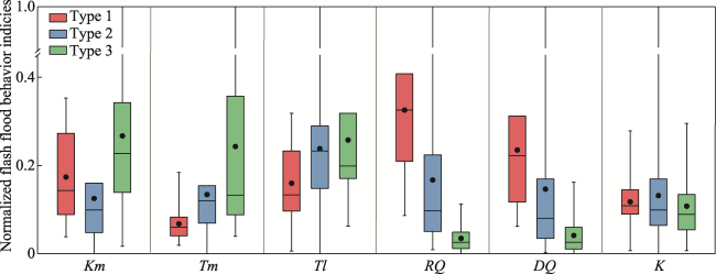
Figure 5 Distribution of normalized flash flood behavior indices induced by three rainfall typesNotes: The flash flood behavior indices are normalized using $Y*=\frac{Y-{{Y}_{\min }}}{{{Y}_{\max }}-{{Y}_{\min }}},$ where Y* and Y are values before and after normalization, respectively; Ymax and Ymin are the maximum and the minimum, respectively. Boxes represent the ranges from the 25th to the 75th quartiles, whiskers represent the ranges from the minimum to the maximum, and dots and lines in boxes represent the averages and the medians, respectively. |
Table 3 Evaluation indices for flash flood process simulation |
| Model | Evaluation indices | Period | Type | |||
|---|---|---|---|---|---|---|
| Calibration | Validation | Type 1 | Type 2 | Type 3 | ||
| XAJ | Absolute RER (%) | 6.89 | 10.62 | 10.73 | 7.67 | 7.81 |
| NSE | 0.78 | 0.72 | 0.79 | 0.71 | 0.85 | |
| CNFF | Absolute RER (%) | 7.58 | 18.58 | 13.17 | 11.00 | 10.60 |
| NSE | 0.87 | 0.70 | 0.76 | 0.81 | 0.85 | |
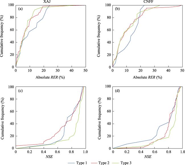
Figure 6 Cumulative frequency distribution of absolute RER and NSE for three rainfall typesNotes: (a) and (c) are the absolute RER and NSE by XAJ, (b) and (d) are the absolute RER and NSE by CNFF. |
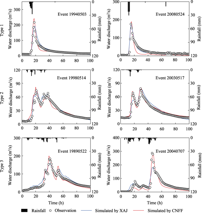
Figure 7 Observed and simulated flash flood processes of partial events |
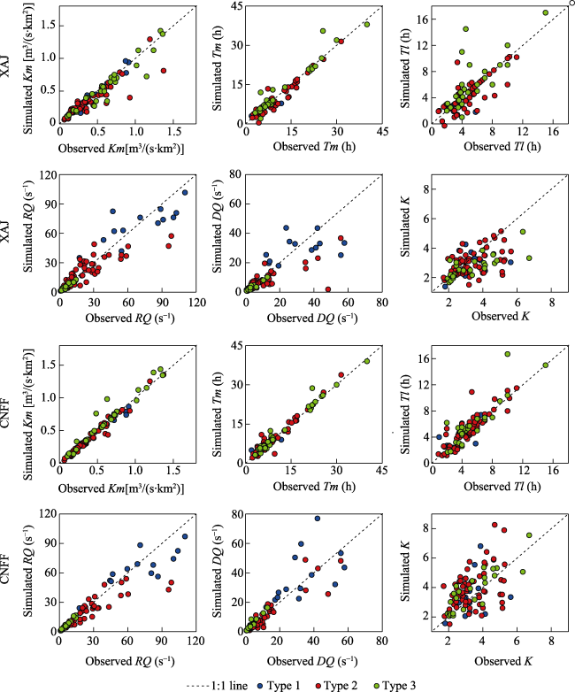
Figure 8 Observed and simulated flash flood behavior indices for XAJ and CNFF |
Table 4 Evaluation indices for flash flood behavior simulations |
| Model | Evaluation indices | Type | Flash flood behavior indices | |||||
|---|---|---|---|---|---|---|---|---|
| Km | Tm | Tl | RQ | DQ | K | |||
| XAJ | RMSEr | Type 1 | 0.15 | 0.26 | 0.35 | 0.27 | 0.44 | 0.35 |
| Type 2 | 0.33 | 0.18 | 0.33 | 0.43 | 0.55 | 0.43 | ||
| Type 3 | 0.18 | 0.18 | 0.49 | 0.23 | 0.33 | 0.33 | ||
| r | Type 1 | 0.96 | 0.89 | 0.70 | 0.79 | 0.46 | 0.23 | |
| Type 2 | 0.90 | 0.96 | 0.85 | 0.85 | 0.85 | 0.39 | ||
| Type 3 | 0.97 | 0.98 | 0.73 | 0.96 | 0.97 | 0.75 | ||
| CNFF | RMSEr | Type 1 | 0.11 | 0.25 | 0.34 | 0.30 | 0.44 | 0.40 |
| Type 2 | 0.12 | 0.16 | 0.29 | 0.36 | 0.55 | 0.36 | ||
| Type 3 | 0.18 | 0.11 | 0.31 | 0.20 | 0.40 | 0.24 | ||
| r | Type 1 | 0.99 | 0.86 | 0.69 | 0.67 | 0.56 | 0.32 | |
| Type 2 | 0.99 | 0.97 | 0.90 | 0.93 | 0.89 | 0.61 | ||
| Type 3 | 0.98 | 0.99 | 0.88 | 0.98 | 0.99 | 0.86 | ||
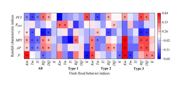
Figure S1 Correlation coefficients between flash flood behavior indices and rainfall characteristic indices for all events and three rainfall types. * indicates the correlation coefficient has a significance level of p<0.05. |
| [1] |
|
| [2] |
|
| [3] |
|
| [4] |
|
| [5] |
|
| [6] |
|
| [7] |
|
| [8] |
|
| [9] |
|
| [10] |
|
| [11] |
|
| [12] |
|
| [13] |
|
| [14] |
|
| [15] |
|
| [16] |
|
| [17] |
|
| [18] |
|
| [19] |
|
| [20] |
|
| [21] |
|
| [22] |
|
| [23] |
|
| [24] |
|
| [25] |
|
| [26] |
|
| [27] |
|
| [28] |
|
| [29] |
|
| [30] |
|
| [31] |
|
| [32] |
Soil Conservation Service, 1972. National Engineering Handbook (Section 4): Hydrology. Washington, DC: US Department of Agriculture.
|
| [33] |
|
| [34] |
|
| [35] |
|
| [36] |
|
| [37] |
|
| [38] |
|
| [39] |
|
| [40] |
|
| [41] |
|
| [42] |
|
| [43] |
|
| [44] |
|
| [45] |
|
| [46] |
|
| [47] |
|
| [48] |
|
/
| 〈 |
|
〉 |