Research Articles

Warm season temperature reconstruction in North China based on the tree-ring blue intensity of Picea meyeri

  • CHEN Qiaomei , 1 ,
  • YUE Weipeng 1 ,
  • CHEN Feng , 1, 2, * ,
  • HADAD Martín 3 ,
  • ROIG Fidel 4, 5 ,
  • ZHAO Xiaoen 1 ,
  • HU Mao 1 ,
  • CAO Honghua 1
Expand
  • 1. Yunnan Key Laboratory of International Rivers and Transboundary Eco-Security, Institute of International Rivers and Eco-Security, Yunnan University, Kunming 650500, China
  • 2. Key Laboratory of Tree-ring Physical and Chemical Research of the Chinese Meteorological Administration/Xinjiang Laboratory of Tree-ring Ecology, Institute of Desert Meteorology, Chinese Meteorological Administration, Urumqi 830002, China
  • 3. Laboratorio de Dendrocronología de Zonas Áridas CIGEOBIO (CONICET-UNSJ), Gabinete de Geología Ambiental (INGEO-UNSJ), San Juan, Argentina
  • 4. Laboratorio de Dendrocronología e Historia Ambiental, IANIGLA-CCT CONICET-Universidad Nacional de Cuyo, Mendoza, Argentina
  • 5. Hémera Centro de Observación de la Tierra, Escuela de Ingeniería Forestal, Facultad de Ciencias, Universidad Mayor, Huechuraba, Santiago, Chile
* Chen Feng, Professor, E-mail:

Chen Qiaomei (1991-), PhD Candidate, E-mail:

Received date: 2022-12-05

  Accepted date: 2023-07-20

  Online published: 2023-12-14

Supported by

National Natural Science Foundation of China(32061123008)

Abstract

In the past 30 years, observational climate datasets reveal a significant a drying and warming trend over in North China. Understanding of climatic variability over North China and its driving mechanism in a long-term perspective is, however, limited to a few sites only, especially the lack of temperature reconstructions based on latewood density and blue intensity. In this study, we developed a 281-year latewood blue intensity chronology based on 45 cores of Picea meyeri in western North China. Based on the discovery that the warm season (May-August) mean maximum temperature is the main controlling factor affecting the change in blue light reflection intensity, we established a regression model that explained 37% of the variance during the calibration period (1950-2020), allowing to trace the mean maximum temperature up to 1760 CE. From the past 261 years, we identified seven persistent high temperature periods (1760-1773, 1778-1796, 1805-1814, 1869-1880, 1889-1934, 1984- 2000, 2004-2020) and three persistent low temperature periods (1815-1868, 1935-1963, 1969-1983) in North China. Comparisons of a nearby temperature reconstructions and climate gridded data indicate that our reconstruction record a wide range of temperature variations in North China. The analysis of links between large-scale climatic variation and the temperature reconstruction showed that there is a relationship between extremes in the warm season temperature and anomalous SSTs in the equatorial eastern Pacific, and implied that the extremes in the warm season temperature in North China will be intensified under future global warming.

Cite this article

CHEN Qiaomei , YUE Weipeng , CHEN Feng , HADAD Martín , ROIG Fidel , ZHAO Xiaoen , HU Mao , CAO Honghua . Warm season temperature reconstruction in North China based on the tree-ring blue intensity of Picea meyeri[J]. Journal of Geographical Sciences, 2023 , 33(12) : 2511 -2529 . DOI: 10.1007/s11442-023-2187-6

1 Introduction

Recent climate warming has become a public concern because of its apparent impact on society, the environment, and various ecosystems (Walther et al., 2002; Morton, 2007; Lafferty, 2009). The ability to study climatic conditions in different regions from a long-term perspective is critical for a comprehensive understanding of current warming (Jones et al., 2004; Zachos et al., 2008; Marcott et al., 2013). Simultaneously, identifying the drivers of temperature change will help to improve the ability to predict future climate change and avoid catastrophic environmental impacts (Jonesand Mann, 2004; Tylianakis et al., 2008; Moss et al., 2010; Zscheischler et al., 2018). The limited observational record, however, limits our comprehensive understanding of climate change in different regions (Zwiers et al., 2013; Sherwood et al., 2020). Long-term regional climate histories can be recovered through a range of climate proxies, and tree rings with high resolution, accurate dating and high replication are among the best indicators of climate change over the past millennium (Yao et al., 1997; Petit et al., 1999; Liu et al., 2011; Maher, 2016; Cheng et al., 2019; Chevalier et al., 2020; Pang et al., 2020; Hadad et al., 2021; Chen et al., 2022a).
The tree-ring width (TRW) and the maximum latewood density (MXD) are particularly important in enhancing the sensitivity of the temperature response and expanding the scope of regional reconstruction (Davi et al., 2003; Chen et al., 2012; Büntgen et al., 2021). However, expensive instruments and complex experimental steps make the extraction of the maximum latewood density index impossible to replicate in each laboratory, while the width also faces the disadvantage of missing temperature signal capture at low altitudes (Campbell et al., 2011; Björklund et al., 2019). Blue intensity (BI) based on high-resolution image technology can effectively compensate for the above shortcomings (Wilson et al., 2014; Wilson et al., 2017; Seftigen et al., 2020; Heeter et al., 2021a, 2021b). It relies on the blue light band reflected by tree ring lignin to derive the relative density parameter of cells, which is relatively simple and inexpensive (Davi et al., 2021; Heeter et al., 2022). Globally, blue intensity has been widely used in the past decade to identify regional tree growth response to climate and reconstruct past temperature (Kaczka et al., 2021), but less research has been done in China (Cao et al., 2022).
North China (approximately 32°N-43°N and 105°E-120°E, Figure 1), one of the densely populated and economically developed regions of the country, plays an important role in ensuring China’s food supply, industrial manufacturing production, and ecological environment balance (Varis et al., 2001; Cai, 2008; Ma et al., 2019). In the context of current climate change, North China is facing a series of severe climate threats, such as high temperatures, drought, forest growth decline, water shortage, and crop yield reduction (Ju et al., 2013; Lei et al., 2016; Xu et al., 2018). Some tree-ring studies have succeeded in obtaining temperature and precipitation data in this area for many centuries based on tree-ring width and hydrogen and oxygen isotopes, but there is no example of reconstructing the mean maximum temperature using the blue intensity parameter (Li et al., 2015; Liu et al., 2019; Cai et al., 2022; Zeng et al., 2022).
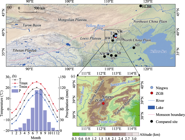
Figure 1 Overview of the study area. (a) The geographical distribution of North China. The pink line is the boundary between the Asian monsoon and the westerly, the black circles are the compared sampling sites, and the blue and red circles are the meteorological station (Ningwu) and the sampling point of this study (ZGB), respectively. (b) The monthly mean temperature (T), monthly mean maximum temperature (Tmax), monthly mean minimum temperature (Tmin) and precipitation (P) at Ningwu meteorological station. (c) Topographic features of the sampling site and the distribution of the water system. All compared samples are from the following papers: Cook et al., (2010); Cai et al., (BWD, 2010); Bao et al., (HLBE, 2012); Li et al., (NW, SD, HS, LY, 2018); Chen et al., (NWT, XF, SR, 2020).
The purpose of this study was to (1) obtain the blue intensity parameters of tree rings, (2) clarify the relationship between changes in tree ring blue intensity and climatic factors, (3) reconstruct the multi-century mean maximum temperature changes in North China, and (4) analyze the driving mechanism of the mean maximum temperature changes.

2 Materials and methods

2.1 Geographical environment and core collection

The study area is located in the north-central part of the Shanxi province, China (Figure 1c), close to Taiyuan, Shijiazhuang and other important industrial cities in North China. Because it is located in the transition zone between humid and arid, corresponding to monsoon and non-monsoon climates, respectively, forest and grassland are environmentally sensitive areas in North China (Li et al., 2011). The temperate continental monsoon climate has obvious characteristics, with four distinct seasons and rainy season overlaps with the warm period (Liu et al., 2013) (Figure 1b). According to the instrumental climate data of the Ningwu meteorological station (112.29°E and 38.99°N, 1409 m a.s.l., 1959-2020, Figure 1a), the total annual precipitation is 454.4 mm, which drops by more than 84% in the warm season (May-September); the annual mean temperature is 6.7℃, and the mean temperatures in January and July are -8.9℃ and 20.7℃, respectively (Figure 1b). Summer (June-August) precipitation originates from water vapor transport over the Pacific Ocean, while the winter (December-February) climate is dominated by cool, dry continental winds (Cai et al., 2010; Li et al., 2015). Snowfall in winter and spring (December-March) supplements water requirements before the growing season (pre-May) (Li et al., 2015). Tree-ring samples were collected from Picea meyeri growing near the timberline in the Guanchen mountain nature reserve (ZGB, 111.9°E and 38.7°N, 2658 m a.s.l., Figure 1c). In October 2020, we drilled 93 wood cores in various locations on 45 living trees using 10 mm diameter increment borers. To eliminate the influence on tree growth from non-climatic factors, we prudently selected healthy stands free from human, fire and insect damages (Speer, 2010). Picea meyeri grows on gentle slopes with sparse stands, and the upper layer of the root system is covered with thick litter.

2.2 Blue intensity chronology development

Changes in the reflection intensity of the blue light band produced by lignin depend on ultra-high-definition image recognition, and subtle errors on the surface of the sample core will affect the measurement results (Rydval et al., 2014). Therefore, we carefully examined all samples in the laboratory to exclude the core of fungal decay, discoloration, traumatic resin duct formation or any other abnormal characteristic signs (Björklund et al., 2014). We soaked the wood cores in hot ethanol for 48 hours using a Soxhlet apparatus and then removed any residual solvent and water-soluble extracts in boiling deionized water to reducing their interference on BI measurements (Poole, 2020; Khan et al., 2022). According to traditional dendrochronological procedures, all sample cores with complete resin removal were fixed by troughs and air-dried at room temperature in the laboratory for 2-3 days (Fritts, 1971). Finally, samples were sanded with progressively finer sandpaper (from 400 to 1000 grit) to obtain a smooth core surface and anatomically visible ring boundaries (Speer, 2010). The transversal surface of most conifers has color differences between sapwood and heartwood (Harley et al., 2021). To reduce the error of blue intensity measurement caused by such color difference, we only used the latewood of Picea meyeri to extract the blue intensity parameter (Seftigen et al., 2020).
We used a flatbed scanner (Epson Expression 12000XL) to complete the rasterization of each core, using 3200-dpi image resolution to achieve accurate identification of latewood boundaries (Wilson et al., 2014; Fuentes et al., 2018; Tsvetanov et al., 2020). To reduce the color interference of visible light on the scanning plane, a simple dark black carton covering the scanner was used and additionally we calibrated images with IT8 calibration software before each scan to reduce color “drift” (Wilson et al., 2014; Fuentes et al., 2018; Tsvetanov et al., 2020). The width of the ring and the blue light reflectivity of the latewood (LWBI) were measured by CooRecorder 9.4 software, and the accuracy of the cross dating was verified with COFECHA program (Grissino-Mayer, 2001; Seftigen et al., 2020; Maxwell et al., 2021). We read 30% of the darkest pixel value on the latewood medium-area surface of each ring as the raw blue intensity (Buckley et al., 2018). To invert the positive relationship between blue intensity and cell density, we set a maximum pixel value of 256 minus the raw blue intensity, which yields the final LWBI measurement (Wilson et al., 2014; 2017).
To avoid the problem of “trend distortion” in low-frequency signals and to eliminate the variability in climate-independent time series, we used RCSsigFree_v45 software to detrend LWBI data (Melvin et al., 2008; Zhang et al., 2017; Qin et al., 2022). Growth trend fitting was first performed using 300-year variable splines (Büntgen et al., 2005), then averaged into a site chronology using the robust weighted mean method, and finally, the variance of the chronology was stabilized using the method described by Osborn et al. (1997). The reliability and strength of the chronological signal were assessed by the mean inter-series correlation (Rbar) and the associated expressed population signal (EPS), calculated from correlation analysis using a 51-year moving window for the chronology and 50-year overlap. The final chronology available for reconstruction was truncated in 1760 because the threshold requirements for EPS ≥ 0.85 and sample depth ≥ 6 were met (Figure 2) (Table 1) (Cook et al., 2010; Chen et al., 2019a; 2022a; 2022b; Yue et al., 2022).
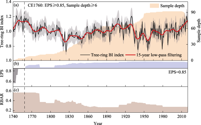
Figure 2 (a) The tree-ring latewood blue intensity standard chronology (LWBI, thin black line), smoothed with a 15-year low-pass filtering (red thick line). Gray shading highlights the ±10% error of the unsmoothed LWBI chronology, and orange fill shows how the sample depth changes over time. (b) Expressed population signal (EPS) (computed over 51 years, lagged by 50 years). (c) Mean inter-series correlation (Rbar) statistics. The EPS > 0.85 threshold is outlined by the vertical dashed line.
Table 1 Tree-ring blue intensity chronology statistics
Parameter MS SD SNR MC VFE AOF EPS MSC EPS≥0.85
ZGB 0.08 0.07 24.25 0.47 24.0% 0.91 0.96 1740-2020 1760

Note: MS: mean sensitivity; SD: standard deviation; SNR: signal-to-noise ratio; MC: mean correlation with master series; VFE: variance in first eigenvector; AOF: autocorrelation order first; EPS: expressed population signal; MSC: master series coverage

2.3 Environmental data and processing methods

The instrumental meteorological data were recorded at the China Meteorological Administration Ningwu station (CMDSC, http://data.cma.cn/en) near the sampling site, including the mean temperature (T), mean maximum temperature (Tmax), mean minimum temperature (Tmin) and precipitation (P). Owing to its short coverage time, we selected the CRU grid climate data as a supplement (CRU TS 4.05, 0.5° × 0.5°, https://crudata.uea.ac.uk/cru/data, Harris et al., 2020), with a spatial range of 38.5°N-39°N and 111.5°E-112.5°E. Response function analysis was performed with all meteorological variables by facilities of Dendroclim 2002 software to estimate the relationship between LWBI chronology and climate (Biondi et al., 2004; Chen et al., 2022a). Due to the lag effect of the response pattern caused by the nutrient supply of the previous year, we extended the response period, including June of the previous year, to December of the current year (Chen et al., 2021). After eliminating the random trend of LWBI and meteorological data by first-order difference calculation, the response analysis is carried out to further examine the stable relationship between the two variables (Blasing et al., 1984). We used Pearson sliding analysis with a 21-year window to verify the stability of the effects of different climatic factors on tree growth in different seasonal combinations and set up a significance test (He et al., 2018).
A simple linear regression function model was developed to convert the LWBI to the mean maximum temperature, with the LWBI as the independent variable and the mean maximum temperature recorded by the instrument as the dependent variable for the entire calibration period (Gou et al., 2013). Leave-one-out cross-validation, including the error reduction test (RE), sign test (ST), product mean test (PMT), and Durbin-Watson test (DW), was used to test the validity of the model (Speer, 2010). According to Liu et al. (2019), the mean ±1σ (σ is the standard deviation) was used to identify warm and cold years, and the mean ±2σ was used for extreme cold and warm events. A 15-year low-pass filtering method (Locally weighted regression, LOWESS, Seftigen et al., 2013) smoothed the reconstructed series, and the smoothed values above (or below) the long-term mean were used to determine warm (or cold) periods (Chen et al., 2019b).
We used the multi-taper method (MTM) and wavelet power spectrum analysis to cross-validate any periodic signal in the temperature recordings and set up a noise test (Mann et al., 2022). To verify the spatial representativeness of the reconstructed mean maximum temperature during the calibration period, four types of data, including instrumental, reconstruction, reconstruction trend removal and reconstruction first-order difference, were used for Pearson spatial correlation analysis with gridded temperature data (Yue et al., 2022). The extended reconstructed sea surface temperature dataset from the National Oceanic and Atmospheric Administration (ERSST, 2°×2°, 1854-2022, http://www.psl.noaa.gov/data/gridded/data.noaa.ersst.v5.html, Huang et al., 2015) (NOAA) was used to analyze the circulation link between the reconstructed mean maximum temperature and the large-scale air-sea circulation, combined with composite mean modal analysis and 850 hPa geopotential height water vapor flux analysis to comprehensively explain the process of heat transfer (Zhou et al., 2005; Moore et al., 2012; Yue et al., 2022).

3 Results

3.1 Linkage between radial growth and climate variables

The correlation between the LWBI chronology and meteorological data was calculated in the common period, including the single-month correlation and seasonal combination correlation from June of the previous year to December of the current year (Figure 3). In general, the LWBI showed a significant positive correlation with the temperature and a weak negative correlation with precipitation in the growing season (March-November) of the current year or the previous year. The seasonal monthly combination correlation verifies the results of the single-month correlation. Whether instrumental meteorological data or grid meteorological data, the results showed that temperature in the warm season (April-August) has the greatest impact on tree growth, with the highest correlation with CRU gridded data between May and August (r = 0.608, p<0.001). Simultaneously, precipitation during summer (June-August, r = -0.354, p<0.01) showed a significant limiting effect on tree growth. The results of sliding correlation analysis showed that the effects of the precipitation on tree growth are not stable, especially after the 1990s. In contrast, the temperature always main-tained a positive relationship with the growth of Picea meyeri, showed relatively strong stability (Figure 3e). The first-order difference method was used to remove the random trend and repeat the above analysis process. We found that the relationship between temperature and LWBI chronology was similar to that before removal, indicating that LWBI chronology stably recorded the temperature signal in North China. At the same time, the negative relationship between winter precipitation and LWBI chronology was significantly enhanced, and the negative relationship between summer precipitation and LWBI chronology was further weakened (Figure 3f).
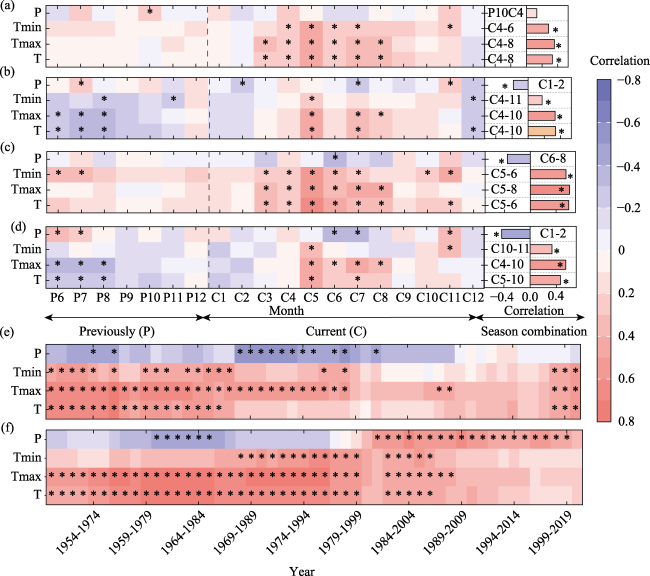
Figure 3 The correlations between the latewood blue intensity chronology (LWBI) and monthly meteorological data (including mean maximum temperature, mean temperature, mean minimum temperature, and total precipitation). Correlation analysis between LWBI and instrumental meteorological data of Ningwu meteorological station is based on the original (a) and first-order difference calculation (b). Correlation analysis between LWBI and CRU grid meteorological data is based on the original (c) and first-order difference calculation (d). The sliding correlation analysis of LWBI and CRU grid data over a 21-year window is based on the original (e) and first-order difference calculations (f). Asterisks (*) indicate the 95% confidence level.

3.2 Warm-season mean maximum temperature reconstruction

The results showed that the warm-season mean maximum temperature is a key controlling factor for LWBI, exhibiting long-term stable effects, and allowing us to reconstruct past dynamics of mean maximum temperature using precisely tree-ring data. A linear regression model was used to reconstruct the history of the mean maximum temperature in the warm season from May to August since 1760 in North China. The reconstruction model based on the entire instrument cycle is Y = 5.12Xi + 16.8, where Y is the mean maximum temperature from May to August, and Xi is the LWBI in year i (Figure 4a). The model explains 37% of the variance in the mean maximum temperature data from 1950 to 2020 (29% after adjusting for the loss of degrees of freedom) (Figure 4b). The statistics of leave-one-out cross- validation are shown in Table 2. RE was positive during both calibration periods, and the results of the sign test, described how well the predicted values tracked the direction of the actual data, also reaching a significant level. DW statistics showed that there is no significant positive autocorrelation between the independent and dependent variables, and the reconstructions and observations during the calibration period from 1950 to 2020 performed well in both low-frequency changes and high-frequency simulations. These results demonstrated that the model used here successfully passes key tests.
Figure 4 The reconstruction process and characteristic analysis of the mean maximum temperature in North China. (a) Scatter plot of LWBI and observed mean maximum temperature from May to August. (b) Original comparison of reconstructed and observed mean maximum temperatures. (c) First-order difference comparison of reconstructed and observed mean maximum air temperature. (d) Reconstruction of the May-August mean maximum temperature of North China since 1760 CE. The black smooth curve was obtained after 15 years of low-pass filtering of the reconstruction results, and the gray dashed and solid lines represent the long-term mean plus or minus the standard deviation. Gray shading was added for ±10% error in the reconstruction results. (e) The distribution of the kernel density function of the observed (pink area) and reconstructed (gray area) mean maximum temperature during the calibration period (1950-2020) and the mean maximum temperature before (light blue area) and after (purple area) the modern warm period (1850) over the whole period (1760-2020). The vertical lines indicate the center of the peak. (f) Results of MTM analysis of the reconstructed results, with the 99% and 95% confidence levels inferred from red noise spectra; periodicities significant at the 99% level are indicated (arrows). (g) Wavelet power spectrum of the reconstructed results, with significant periods (p < 0.05) highlighted by black lines.
Table 2 Leave-one-out cross-validation statistics for the warm-season mean maximum temperature reconstructions
Calibration Validation
Period R2 Radj2 F Period RE PMT ST DW
1986-2020 0.270 0.248 12.23** 1950-1985 0.216 5.035 22+/14-** 2.064
1950-1985 0.295 0.275 14.29** 1986-2020 0.182 4.484 23+/12-** 1.718
1950-2020 0.369 0.360 40.51**

Note: R2: model explained variance, Radj2: adjusted R2 considering multiple independent variables in the model, F: statistical significance of the regression model, DW: Durbin-Watson test, RE: reduction of error, ST: sign test, PMT: product means test. ** indicates the 99% confidence level.

3.3 Warm-season mean maximum temperature variability

The long-term mean for the 261-year mean maximum temperature is 21.9℃ with a standard deviation of 0.46℃. A total of 7 persistent high-temperature periods (1760-1773, 1778-1796, 1805-1814, 1869-1880, 1889-1934, 1984-2000, 2004-2020) and 3 persistent low-temperature periods (1815-1868, 1935-1963, 1969-1983) was observed on the decadal scale (Figure 4d). In terms of interannual high and low temperature changes, there are a total of 41 high temperature years and 40 low temperature years, among which 1761, 1909, 1929, 1930, 1931, and 2018 are defined as extremely high temperature years, while 1820, 1821, 1824, 1825, 1940, 1956, 1979, and 1988 are defined as extremely low temperature years (Figure 4d). In general, after the end of the Little Ice Age (LIA, 1250-1850), the incidence of extreme weather events, including high temperatures and droughts, increased significantly as evidenced in Figure 4e. The kernel density distribution map showed that the distribution density of high temperatures in the period after 1850 is skewed to the right, especially in the calibration period (1950-2020). The results of MTM and wavelet power spectrum analysis cross-validated that the reconstructed mean maximum temperature has the characteristics of interannual and interdecadal periodic recurrence, especially 2.0-2.5 (99%), 7.6-7.7 (95%), and 20-23.2 (95%). At the same time, we also noticed the characteristic of increased cycle recurrence approximately 2-7 years after 1850 (Figures 4f and 4g).

4 Discussion

4.1 Warm-season temperature signals recorded by tree-ring blue intensity

There was a significant negative correlation between BI and MXD (r > 0.95, p < 0.0001) because both were essentially measurements of cellulose and lignin in tree rings (Wilson et al., 2017; Nagavciuc et al., 2019). The blue light band in the synthetic spectrum is extremely efficient for the light reflection intensity of lignin, which is based on the proliferation of cell numbers and the thickening of the cell wall (Campbell et al., 2007). Therefore, compared with the tree ring width and the maximum latewood density, the dense and dark LWBI expresses a “more pure” climatic signal and is less affected by specific non-climatic factors detected in other locations (Wilson et al., 2017). It has been observed that the growth of conifers in the upper timberline is sensitive to temperature response, especially during the warm season (May-September). This includes Pinus sylvestris in high latitudes, Juniperus rigida and Picea schrenkiana in the Tibetan Plateau, Pinus tabuliformis in arid regions, etc. The tree species selected for this study also follow this rule (Chen et al., 2009; Bao et al., 2012; Tipton et al., 2016; Zhao et al., 2019). Temperatures during the growing season (March to November) are prime for conifer cell division and expansion, with snowmelt and soil warming promoting faster growth of leaf buds and stems (Shibistova et al., 2002; Yu et al., 2013). The latewood cell density becomes thicker after the season. The content of lignin depends on the increase in the density of cells, and the high content of lignin reduces the reflection intensity of blue light, so the blue intensity and density maintain a significant negative relationship, being a positive and significant relationship after making the correction of the formula (Kozlowski et al., 1991; Ernakovich et al., 2014; Heeter et al., 2021a). In contrast, the precipitation during the monsoon season (June-August) and winter (January-February) increases cloud cover, weakens the total solar radiation, increases the shallow soil moisture, expands the growth ring cells, thins the cell wall, and enhances the blue light reflection efficiency due to the lignin content (Björklund et al., 2014). Thus, the blue intensity corrected by the formula maintains a negative relationship with precipitation.

4.2 Links to large-scale hydroclimate

To test and understand the spatial representativeness of our reconstruction, we performed spatial correlations between the temperature reconstruction and the CRU grid dataset during the calibration period between 1950 and 2020. Figure 5 shows that the reconstructed results and the observed data have very similar patterns and pass the significance test (99%), indicating that our temperature reconstruction can represent large-scale climate variability and change. Additionally, we also noted that the significant spatial correlation mainly covers the three geographical regions of the North China Plain (32°N-40°N and 114°E-121°E), Loess Plateau (33°N-41°N and 100°E-114°E) and Desert Gobi (37°N-45°N and 100°E-115°E), which are facing a series of complex climate change problems, such as water shortages, fragile ecosystems, and low extreme climate adaptability (Liu et al., 2013; Li et al., 2015; Li et al., 2018). To evaluate whether our reconstruction results also have large-scale spatial hydroclimate signals before the calibration period, five hydroclimate series reconstructed based on tree-ring proxy data were collected in North China, three of which were temperature reconstruction (Cai et al., 2010; Bao et al., 2012; Li et al., 2018), and the other two were drought or streamflow reconstruction (Cook et al., 2010; Chen et al., 2020).
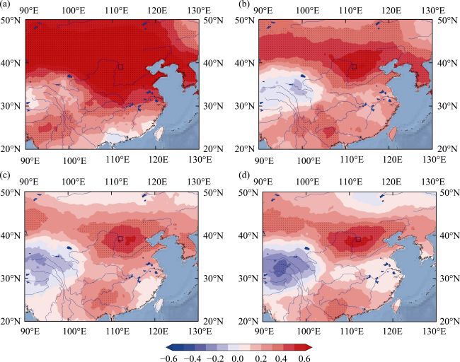
Figure 5 Spatially correlated between CRU gridded climate data from May to August for the 1950-2020 period with (a) observed mean maximum temperature, (b) reconstructed mean maximum temperature, (c) detrended mean maximum temperature, (d) first-order difference of mean maximum temperature. A black square indicates the extent of the study area, marked by 95% of the area covered by black dots as a comparison marker.
The comparison of temperature reconstructions in different regions shows that North China has experienced a rapid warming trend since 1956, which is unprecedented in the past two centuries (Figure 6). At the same time, three common continuous high-temperature period signals were also captured, which appeared in 1832-1843, 1905-1911, and 1926-1934 respectively, which indicates that the spatial pattern of temperature changes in North China remains consistent from south to north (Cai et al., 2010; Bao et al., 2012; Li et al., 2018) (Figure 6). The negative correlation occurs between the mean maximum temperature and the drought index or streamflow, indicating that sustained high temperature may trigger meteorological drought and thus conduct hydrological drought (Huang et al., 2017). For example, in 1760-1767, 1807-1816, 1924-1933, and 1992-2020, the high temperature in North China corresponds to the drought and the low runoff period of the Yellow River (Figure 6). The climatic and hydrological drought caused by the continuous high temperature undoubtedly caused enormous damage to the social economy and loss of life, especially in North China during the 1920s to 1930s (Qian et al., 2001; Liang et al., 2006; Qian et al., 2007; Fang et al., 2009). However, with the improvement of social productivity, we can maintain a good adaptation to the pressure brought by drought, especially in the context of extremely climatic and hydrological changes brought about by global warming. Water conservancy projects such as the South-to-North Water Diversion have greatly improved our ability to cope with climate change (Zhao et al., 2017; Zhang et al., 2018).
Figure 6 Comparison of the present reconstruction of the mean maximum temperature (May to August) with other paleoclimatic records derived from tree-ring from surrounding regions. (a) Reconstruction of mean maximum temperature from May to August in North China (this study). (b) Reconstruction of mean temperature from May to August in northern-central China (Li et al., 2018). (c) Reconstruction of mean maximum temperature from April to September in Hulunbuir, Inner Mongolia (Bao et al., 2012). (d) Reconstruction of mean temperature from May to July in Lüliang Mountain, Shanxi (Cai et al., 2010). (e) Regional PDSI reconstruction for North China (Cook et al., 2010). (f) Summer monsoon season (July to October) streamflow variation reconstruction for the middle Yellow River (Chen et al., 2020). All sequences are dimensionless and standardized by the Z score, and low-frequency fluctuations are realized by the low-pass filtering method (LOWESS) with a 10-year step size. On the basis of the mean value, all series are filled upward (downward) as red, indicating a warm period (dry period or low streamflow period), while downward (upward) as blue indicates a cold period (wet period or high streamflow period). The common warm period (dry period or low streamflow period) is marked with an orange square, and the common cold period (wet period or high streamflow period) is marked with a purple square.

4.3 Links to atmospheric circulations

The results of the periodic analysis showed that our reconstructed mean maximum temperature in the warm season has a significant 2-7-year cycle, which may be related to the mid- and low-latitude Pacific SST anomalies. Regarding the mechanism of this relationship, we analyzed the spatial correlation pattern between the calibration period (1950-2020) and the ERSST sea surface temperature dataset, results that are shown in Figure 7. We found that the significant correlation fields between the original reconstruction and SST are mainly concentrated in the Pacific Ocean, Indian Ocean and Atlantic Ocean, which are also the main heat sources of traditional land-sea heat exchange (Mohtadi et al., 2016). However, after removing the linear trend by the first-order difference, the main significant positive correlation fields are concentrated on the east coast of the low-latitude Pacific Ocean, which is also the main monitoring area of the Niño 3 index (Ren et al., 2011). Through the correlation calculation with the Niño 3 index from May to August, there is a significant positive correlation between the two (r = 0.21, p<0.01, 1871-2020, not shown).
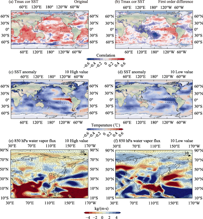
Figure 7 Spatial correlation and composite analysis. (a) The original reconstruction is spatially correlated with the SST during the calibration period. (b) The first-order difference of reconstruction is spatially correlated with the SST during the calibration period. (c) Composite modes of SST corresponding to 10 high-temperature years during the calibration period. (d) Composite modes of SST corresponding to 10 low-temperature years during the calibration period. (e) Composite modes of the water vapor flux divergence corresponding to 10 high-temperature years during the calibration period. (f) Composite modes of the water vapor flux divergence corresponding to 10 low-temperature years during the calibration period.
The composite analysis revealed how the Pacific SSTA affects the dynamic mechanism of the mean maximum temperature change in North China. We selected 10 high-temperature years and 10 low-temperature years for sea surface temperature and water vapor flux divergence synthesis analysis. When a high-temperature year occurs, the sea temperature region indicated by the Niño 3 index is in a warm phase and forms an El Niño mode. At this time, the monsoon rain belt lags behind the South China Sea and the Indochina Peninsula. North China is under the control of the subtropical high-pressure zone, with prevailing sinking airflow and inland wind, dry and little rain, and frequent high-temperature weather (Ding, 1992). In contrast, when a low-temperature year occurs, the sea temperature region indicated by the Niño 3 index is in the cold phase and forms the La Niña mode. The Asian monsoon is strong, the rainfall in North China is greater, and the increase in cloud amount absorbs the heat radiation of the sun and the ground to reduce the temperature (Wang et al., 2017).

5 Conclusions

Herein, we have shown that the latewood blue light intensity (LWBI) resulted in the increased climate information and warm season temperature reconstruction from the tree rings of Picea meyeri in North China that has very few high-resolution temperature records. This is the first LWBI chronology of spruce (Picea meyeri) developed from North China and it has captured the recent warming trend indicated by the instrumental climate data. The reconstructed average maximum temperature represents a large-scale spatial signal, covering typical areas of water shortage in North China, and suggests an out-of-phase relationship between the temperature reconstruction and the hydroclimate reconstructions over past 200 years. Synoptic climatology analysis indicated that the sea surface temperature anomaly on eastern tropical Pacific Ocean play a role in modulating temperature variations in the study area. Additional data from North China is necessary to substantiate these findings.
[1]
Bao G, Liu Y, Linderholm H W, 2012. April-September mean maximum temperature inferred from Hailar pine (Pinus sylvestris var. mongolica) tree rings in the Hulunbuir region, Inner Mongolia, back to 1868AD. Palaeogeography, Palaeoclimatology, Palaeoecology, 313/314: 162-172.

DOI

[2]
Biondi F, Waikul K, 2004. DENDROCLIM2002: A C++ program for statistical calibration of climate signals in tree-ring chronologies. Computers & Geosciences, 30(3): 303-311.

DOI

[3]
Björklund J, von Arx G, Nievergelt D et al., 2019. Scientific merits and analytical challenges of tree-ring densitometry. Reviews of Geophysics, 57(4): 1224-1264.

DOI

[4]
Björklund J A, Gunnarson B E, Seftigen K et al., 2014. Blue intensity and density from northern Fennoscandian tree rings, exploring the potential to improve summer temperature reconstructions with earlywood information. Climate of the Past, 10(2): 877-885.

DOI

[5]
Blasing T J, Solomon A M, Duvick D N, 1984. Response functions revisited. Tree-Ring Bulletin, 44: 1-15.

[6]
Buckley B M, Hansen K G, Griffin K L et al., 2018. Blue intensity from a tropical conifer’s annual rings for climate reconstruction: An ecophysiological perspective. Dendrochronologia, 50: 10-22.

DOI

[7]
Büntgen U, Esper J, Frank D C et al., 2005. A 1052-year tree-ring proxy for alpine summer temperatures. Climate Dynamics, 25(2): 141-153.

DOI

[8]
Büntgen U, Urban O, Krusic P J et al., 2021. Recent European drought extremes beyond Common Era background variability. Nature Geoscience, 14(4): 190-196.

DOI

[9]
Cai Q, Liu Y, Bao G et al., 2010. Tree-ring-based May-July mean temperature history for Lüliang Mountains, China, since 1836. Chinese Science Bulletin, 55: 3008-3014.

DOI

[10]
Cai Q, Liu Y, Fang C et al., 2022. Insight into spatial-temporal patterns of hydroclimate change on the Chinese Loess Plateau over the past 250 years, using new evidence from tree rings. Science of The Total Environment, 850: 157960.

DOI

[11]
Cai X, 2008. Water stress, water transfer and social equity in northern China: Implications for policy reforms. Journal of Environmental Management, 87(1): 14-25.

DOI

[12]
Campbell R, McCarroll D, Loader N J et al., 2007. Blue intensity in Pinus sylvestris tree-rings: Developing a new palaeoclimate proxy. The Holocene, 17(6): 821-828.

DOI

[13]
Campbell R, McCarroll D, Robertson I et al., 2011. Blue intensity in Pinus sylvestris tree rings: A manual for a new palaeoclimate proxy. Tree-Ring Research, 67(2): 127-134.

DOI

[14]
Cao X, Hu H, Kao P K et al., 2022. Improved spring temperature reconstruction using earlywood blue intensity in southeastern China. International Journal of Climatology, 42(12): 6204-6220.

DOI

[15]
Chen F, Hadad M, Zhao X et al., 2022a. Abnormally low precipitation-induced ecological imbalance contributed to the fall of the Ming Dynasty: New evidence from tree rings. Climatic Change, 173(1): 13.

DOI

[16]
Chen F, Opała-Owczarek M, Khan A et al., 2021. Late twentieth century rapid increase in high Asian seasonal snow and glacier-derived streamflow tracked by tree rings of the upper Indus River basin. Environmental Research Letters, 16(9): 094055.

DOI

[17]
Chen F, Opała-Owczarek M, Owczarek P et al., 2020. Summer monsoon season streamflow variations in the Middle Yellow River since 1570 CE inferred from tree rings of Pinus tabulaeformis. Atmosphere, 11(7): 717.

DOI

[18]
Chen F, Shang H M, Panyushkina I et al., 2019a. 500-year tree-ring reconstruction of Salween River streamflow related to the history of water supply in Southeast Asia. Climate Dynamics, 53(11): 6595-6607.

DOI

[19]
Chen F, Yuan Y, Trouet V et al., 2022b. Ecological and societal effects of Central Asian streamflow variation over the past eight centuries. NPJ Climate and Atmospheric Science, 5(1): 27.

DOI

[20]
Chen F, Yuan Y, Wei W et al., 2012. Tree ring density-based summer temperature reconstruction for Zajsan Lake area, East Kazakhstan. International Journal of Climatology, 32(7): 1089-1097.

DOI

[21]
Chen F, Yuan Y, Yu S et al., 2019b. A 391-year summer temperature reconstruction of the Tien Shan, reveals far-reaching summer temperature signals over the midlatitude Eurasian Continent. Journal of Geophysical Research: Atmospheres, 124(22): 11850-11862.

[22]
Chen J, Wang L, Zhu H et al., 2009. Reconstructing mean maximum temperature of growing season from the maximum density of the Schrenk spruce in Yili, Xinjiang, China. Chinese Science Bulletin, 54(13): 2300-2308.

DOI

[23]
Cheng H, Zhang H, Zhao J et al., 2019. Chinese stalagmite paleoclimate researches: A review and perspective. Science China Earth Sciences, 62(10): 1489-1513.

DOI

[24]
Chevalier M, Davis B A S, Heiri O et al., 2020. Pollen-based climate reconstruction techniques for late Quaternary studies. Earth-Science Reviews, 210: 103384.

DOI

[25]
Cook E R, Anchukaitis K J, Buckley B M et al., 2010. Asian monsoon failure and megadrought during the last millennium. Science, 328(5977): 486-489.

DOI PMID

[26]
Davi N K, Jacoby G C, Wiles G C, 2003. Boreal temperature variability inferred from maximum latewood density and tree-ring width data, Wrangell Mountain region, Alaska. Quaternary Research, 60(3): 252-262.

DOI

[27]
Davi N K, Rao M P, Wilson R et al., 2021. Accelerated recent warming and temperature variability over the past eight centuries in the Central Asian Altai from blue intensity in tree rings. Geophysical Research Letters, 48(16): e2021GL092933.

[28]
Ding Y, 1992. Summer monsoon rainfalls in China. Journal of the Meteorological Society of Japan (Ser. II), 70(1B): 373-396.

[29]
Ernakovich J G., Hopping K A, Berdanier A B et al., 2014. Predicted responses of Arctic and alpine ecosystems to altered seasonality under climate change. Global Change Biology, 20(10): 3256-3269.

DOI PMID

[30]
Fang K, Gou X, Chen F et al., 2009. Drought variations in the eastern part of northwest China over the past two centuries: Evidence from tree rings. Climate Research, 38(2): 129-135.

DOI

[31]
Fritts H C, 1971. Dendroclimatology and dendroecology. Quaternary Research, 1(4): 419-449.

DOI

[32]
Fuentes M, Salo R, Björklund J et al., 2018. A 970-year-long summer temperature reconstruction from Rogen, west-central Sweden, based on blue intensity from tree rings. The Holocene, 28(2): 254-266.

DOI

[33]
Gou X, Yang T, Gao L et al., 2013. A 457-year reconstruction of precipitation in the southeastern Qinghai-Tibet Plateau, China using tree-ring records. Chinese Science Bulletin, 58(10): 1107-1114.

DOI

[34]
Grissino-Mayer H D, 2001. Evaluating crossdating accuracy: A manual and tutorial for the computer program COFECHA. Tree-Ring Research, 57(2): 205-221.

[35]
Hadad M A, González-Reyes Á, Roig F A et al., 2021. Tree-ring-based hydroclimatic reconstruction for the northwest Argentine Patagonia since 1055 CE and its teleconnection to large-scale atmospheric circulation. Global and Planetary Change, 202: 103496.

DOI

[36]
Harley G L, Heeter K J, Maxwell J T et al., 2021. Towards broad-scale temperature reconstructions for Eastern North America using blue light intensity from tree rings. International Journal of Climatology, 41(Suppl.1): E3142-E3159.

[37]
Harris I, Osborn T J, Jones P et al., 2020. Version 4 of the CRU TS monthly high-resolution gridded multivariate climate dataset. Scientific Data, 7(1): 109.

DOI PMID

[38]
He M, Bräuning A, Grießinger J et al., 2018. May-June drought reconstruction over the past 821 years on the south-central Tibetan Plateau derived from tree-ring width series. Dendrochronologia, 47: 48-57.

DOI

[39]
Heeter K J, Harley G L, Maxwell J T et al., 2021a. Summer temperature variability since 1730 CE across the low-to-mid latitudes of western North America from a tree ring blue intensity network. Quaternary Science Reviews, 267: 107064.

DOI

[40]
Heeter K J, King D J, Harley G L et al., 2022. Video tutorial: Measuring blue intensity with the CooRecorder software application. Dendrochronologia, 76: 125999.

DOI

[41]
Heeter K J, Rochner M L, Harley G L, 2021b. Summer air temperature for the Greater Yellowstone Ecoregion (770-2019 CE) over 1,250 years. Geophysical Research Letters, 48(7): e2020GL092269.

[42]
Huang B, Banzon V F, Freeman E et al., 2015. Extended Reconstructed Sea Surface Temperature Version 4 (ERSST.v4) (Part I): Upgrades and intercomparisons. Journal of climate, 28(3): 911-930.

DOI

[43]
Huang S, Li P, Huang Q et al., 2017. The propagation from meteorological to hydrological drought and its potential influence factors. Journal of Hydrology, 547: 184-195.

DOI

[44]
Jones P D, Mann M E, 2004. Climate over past millennia. Reviews of Geophysics, 42(2): RG2002.

[45]
Ju H, van der Velde M, Lin E et al., 2013. The impacts of climate change on agricultural production systems in China. Climatic Change, 120(1): 313-324.

DOI

[46]
Kaczka R J, Wilson R, 2021. I-BIND: International Blue intensity network development working group. Dendrochronologia, 68: 125859.

DOI

[47]
Khan R, Jolly R, Fatima T et al., 2022. Extraction processes for deriving cellulose: A comprehensive review on green approaches. Polymers for Advanced Technologies, 33(7): 2069-2090.

DOI

[48]
Kozlowski T T, Kramer P J, Pallardy S G, 1991. The physiological ecology of woody plants. Tree Physiology, 8(2): 213-213.

[49]
Lafferty K D, 2009. The ecology of climate change and infectious diseases. Ecology, 90(4): 888-900.

DOI PMID

[50]
Lei Y, Zhang H, Chen F et al., 2016. How rural land use management facilitates drought risk adaptation in a changing climate: A case study in arid northern China. Science of The Total Environment, 550: 192-199.

DOI

[51]
Li Q, Liu Y, Nakatsuka T et al., 2015. The 225-year precipitation variability inferred from tree-ring records in Shanxi province, the North China, and its teleconnection with Indian summer monsoon. Global and Planetary Change, 132: 11-19.

DOI

[52]
Li Q, Liu Y, Zhao B et al., 2018. Temperature variability in North-Central China during the past 231 years based on multiple proxies. Quaternary International, 487: 26-32.

DOI

[53]
Li Q, Nakatsuka T, Kawamura K et al., 2011. Hydroclimate variability in the North China Plain and its link with El Niño-Southern Oscillation since 1784 A.D.: Insights from tree-ring cellulose δ18O. Journal of Geophysical Research: Atmospheres, 116(D22).

[54]
Liang E, Liu X, Yuan Y et al., 2006. The 1920s drought recorded by tree rings and historical documents in the semi-arid and arid areas of northern China. Climatic Change, 79(3): 403-432.

DOI

[55]
Liu J, Chen F, Chen J et al., 2011. Humid medieval warm period recorded by magnetic characteristics of sediments from Gonghai Lake, Shanxi, North China. Chinese Science Bulletin, 56(23): 2464-2474.

DOI

[56]
Liu Y, Wang L, Li Q et al., 2019. Asian summer monsoon-related relative humidity recorded by tree ring δ18O during last 205 years. Journal of Geophysical Research: Atmospheres, 124(17/18): 9824-9838.

[57]
Liu Y, Wang Y, Li Q et al., 2013. Reconstructed May-July mean maximum temperature since 1745AD based on tree-ring width of Pinus tabulaeformis in Qianshan Mountain, China. Palaeogeography, Palaeoclimatology, Palaeoecology, 388: 145-152.

DOI

[58]
Ma L, Long H, Zhang Y et al., 2019. Agricultural labor changes and agricultural economic development in China and their implications for rural vitalization. Journal of Geographical Sciences, 29(2): 163-179.

DOI

[59]
Maher B A, 2016. Palaeoclimatic records of the loess/palaeosol sequences of the Chinese Loess Plateau. Quaternary Science Reviews, 154: 23-84.

DOI

[60]
Mann M E, Steinman B A, Brouillette D J et al., 2022. On the estimation of internal climate variability during the preindustrial past millennium. Geophysical Research Letters, 49(2): e2021GL096596.

[61]
Marcott S A, Shakun J D, Clark P U et al., 2013. A reconstruction of regional and global temperature for the past 11,300 years. Science, 339(6124): 1198-1201.

DOI PMID

[62]
Maxwell R S, Larsson L A, 2021. Measuring tree-ring widths using the CooRecorder software application. Dendrochronologia, 67: 125841.

DOI

[63]
Melvin T M, Briffa K R, 2008. A “signal-free” approach to dendroclimatic standardisation. Dendrochronologia, 26(2): 71-86.

DOI

[64]
Mohtadi M, Prange M, Steinke S, 2016. Palaeoclimatic insights into forcing and response of monsoon rainfall. Nature, 533(7602): 191-199.

DOI

[65]
Moore B J, Neiman P J, Ralph F M et al., 2012. Physical processes associated with heavy flooding rainfall in Nashville, Tennessee, and vicinity during 1-2 May 2010: The role of an atmospheric river and mesoscale convective systems. Monthly Weather Review, 140(2): 358-378.

DOI

[66]
Morton J F, 2007. The impact of climate change on smallholder and subsistence agriculture. Proceedings of the National Academy of Sciences, 104(50): 19680-19685.

DOI

[67]
Moss R H, Edmonds J A, Hibbard K A et al., 2010. The next generation of scenarios for climate change research and assessment. Nature, 463(7282): 747-756.

DOI

[68]
Nagavciuc V, Roibu C C, Ionita M et al., 2019. Different climate response of three tree ring proxies of Pinus sylvestris from the Eastern Carpathians, Romania. Dendrochronologia, 54: 56-63.

DOI

[69]
Osborn T J, Biffa K, Jones P, 1997. Adjusting variance for sample-size in tree-ring chronologies and other regional mean timeseries. Dendrochronologia, 15: 89-99.

[70]
Pang H, Hou S, Zhang W et al., 2020. Temperature trends in the northwestern Tibetan Plateau constrained by ice core water isotopes over the past 7,000 years. Journal of Geophysical Research: Atmospheres, 125(19): e2020JD032560.

[71]
Petit J R, Jouzel J, Raynaud D et al., 1999. Climate and atmospheric history of the past 420,000 years from the Vostok ice core, Antarctica. Nature, 399(6735): 429-436.

DOI

[72]
Poole C F, 2020. Chapter 1: Milestones in the development of liquid-phase extraction techniques. Liquid-Phase Extraction, 1-44.

[73]
Qian W, Lin X, Zhu Y et al., 2007. Climatic regime shift and decadal anomalous events in China. Climatic Change, 84(2): 167-189.

DOI

[74]
Qian W, Zhu Y, 2001. Climate change in China from 1880 to 1998 and its impact on the environmental condition. Climatic Change, 50(4): 419-444.

DOI

[75]
Qin L, Liu K, Shang H et al., 2022. Minimum temperature during the growing season limits the radial growth of timberline Schrenk spruce (P. schrenkiana). Agricultural and Forest Meteorology, 322: 109004.

[76]
Ren H L, Jin F F, 2011. Niño indices for two types of ENSO. Geophysical Research Letters, 38(4): L04704.

[77]
Rydval M, Larsson L Å, McGlynn L et al., 2014. Blue intensity for dendroclimatology: Should we have the blues? Experiments from Scotland. Dendrochronologia, 32(3): 191-204.

DOI

[78]
Seftigen K, Fuentes M, Ljungqvist F C et al., 2020. Using blue intensity from drought-sensitive Pinus sylvestris in Fennoscandia to improve reconstruction of past hydroclimate variability. Climate Dynamics, 55(3): 579-594.

DOI

[79]
Seftigen K, Linderholm H W, Drobyshev I et al., 2013. Reconstructed drought variability in southeastern Sweden since the 1650s. International Journal of Climatology, 33(11): 2449-2458.

DOI

[80]
Sherwood S C, Webb M J, Annan J D et al., 2020. An assessment of earth’s climate sensitivity using multiple lines of evidence. Reviews of Geophysics, 58(4): e2019RG000678.

[81]
Shibistova O, Lloyd J, Zrazhevskaya G et al., 2002. Annual ecosystem respiration budget for a Pinus sylvestris stand in central Siberia. Tellus B: Chemical and Physical Meteorology, 54(5): 568-589.

DOI

[82]
Speer J H, 2010. Fundamentals of Tree-ring Research. University of Arizona Press.

[83]
Tipton J, Hooten M, Pederson N et al., 2016. Reconstruction of late Holocene climate based on tree growth and mechanistic hierarchical models. Environmetrics, 27(1): 42-54.

DOI

[84]
Tsvetanov N, Dolgova E, Panayotov M, 2020. First measurements of blue intensity from Pinus peuce and Pinus heldreichii tree rings and potential for climate reconstructions. Dendrochronologia, 60: 125681.

DOI

[85]
Tylianakis J M, Didham R K, Bascompte J et al., 2008. Global change and species interactions in terrestrial ecosystems. Ecology Letters, 11(12): 1351-1363.

DOI PMID

[86]
Varis O, Vakkilainen P, 2001. China’s 8 challenges to water resources management in the first quarter of the 21st century. Geomorphology, 41(2): 93-104.

DOI

[87]
Walther G R, Post E, Convey P et al., 2002. Ecological responses to recent climate change. Nature, 416(6879): 389-395.

DOI

[88]
Wang P X, Wang B, Cheng H et al., 2017. The global monsoon across time scales: Mechanisms and outstanding issues. Earth-Science Reviews, 174: 84-121.

DOI

[89]
Wilson R, Rao R, Rydval M et al., 2014. Blue Intensity for dendroclimatology: The BC blues: A case study from British Columbia, Canada. The Holocene, 24(11): 1428-1438.

DOI

[90]
Wilson R, Wilson D, Rydval M et al., 2017. Facilitating tree-ring dating of historic conifer timbers using blue intensity. Journal of Archaeological Science, 78: 99-111.

DOI

[91]
Xu H J, Wang X P, Zhao C Y et al., 2018. Diverse responses of vegetation growth to meteorological drought across climate zones and land biomes in northern China from 1981 to 2014. Agricultural and Forest Meteorology, 262: 1-13.

DOI

[92]
Yao T, Thompson L G et al., 1997. Climate variation since the Last Interglaciation recorded in the Guliya ice core. Science in China Series D: Earth Sciences, 40(6): 662-668.

DOI

[93]
Yu S, Yuan Y, Wei W et al., 2013. A 352-year record of summer temperature reconstruction in the western Tianshan Mountains, China, as deduced from tree-ring density. Quaternary Research, 80(2): 158-166.

DOI

[94]
Yue W, Zhao X, Chen F et al., 2022. Reconstructed precipitation in the Lohit River basin, southern Tibetan Plateau since 1720 CE and its weak linkages with monsoon-season Brahmaputra discharge. International Journal of Climatology, 42(7): 3793-3808.

DOI

[95]
Zachos J C, Dickens G R, Zeebe R E, 2008. An early Cenozoic perspective on greenhouse warming and carbon-cycle dynamics. Nature, 451(7176): 279-283.

DOI

[96]
Zeng X, Liu Y, Song H et al., 2022. Tree-ring-based drought variability in northern China over the past three centuries. Journal of Geographical Sciences, 32(2): 214-224.

DOI

[97]
Zhang E, Yin X A, Xu Z et al., 2018. Bottom-up quantification of inter-basin water transfer vulnerability to climate change. Ecological Indicators, 92: 195-206.

DOI

[98]
Zhang Y, Tian Q, Guillet S et al., 2017. 500-yr. precipitation variability in southern Taihang Mountains, China, and its linkages to ENSO and PDO. Climatic Change, 144(3): 419-432.

DOI

[99]
Zhao Y, Shi J, Shi S et al., 2019. Early summer hydroclimatic signals are captured well by tree-ring earlywood width in the eastern Qinling Mountains, central China. Climate of the Past, 15(3): 1113-1131.

DOI

[100]
Zhao Z Y, Zuo J, Zillante G, 2017. Transformation of water resource management: A case study of the South-to-North Water Diversion project. Journal of Cleaner Production, 163: 136-145.

DOI

[101]
Zhou T J, Yu R C, 2005. Atmospheric water vapor transport associated with typical anomalous summer rainfall patterns in China. Journal of Geophysical Research: Atmospheres, 110: D08104.

[102]
Zscheischler J, Westra S, van den Hurk B J J M et al., 2018. Future climate risk from compound events. Nature Climate Change, 8(6): 469-477.

DOI

[103]
Zwiers F W, Alexander L V, Hegerl G C et al., 2013. Climate extremes: Challenges in estimating and understanding recent changes in the frequency and intensity of extreme climate and weather events. In: Asrar G R, Hurrell J W ed. Climate Science for Serving Society: Research, Modeling and Prediction Priorities. Springer: Dordrecht, Netherlands, 339-389.

Outlines

/