Research Articles

Spatio-temporal prediction of regional land subsidence via ConvLSTM

  • LENG Jing , 1, 2, 3 ,
  • GAO Mingliang , 1, 2, 3, 4, * ,
  • GONG Huili 1, 2, 3, 4 ,
  • CHEN Beibei 1, 2, 3, 4 ,
  • ZHOU Chaofan 1, 2, 3, 4 ,
  • SHI Min 5 ,
  • CHEN Zheng 6 ,
  • LI Xiang 1, 2, 3
Expand
  • 1. Beijing Laboratory of Water Resources Security, Capital Normal University, Beijing 100048, China
  • 2. Key Laboratory of Mechanism, Prevention and Mitigation of Land Subsidence, MOE, Capital Normal University, Beijing 100048, China
  • 3. College of Resources Environment and Tourism, Capital Normal University, Beijing 100048, China
  • 4. Hebei Cangzhou Groundwater and Land Subsidence National Observation and Research Station, Cangzhou 061000, Hebei, China
  • 5. School of Electrical Engineering, Nantong University, Nantong 226019, Jiangsu, China
  • 6. Technical Centre for Soil, Agriculture and Rural Ecology and Environment, Ministry of Ecology and Environment, Beijing 100012, China
*Gao Mingliang (1989-), Lecturer, specialized in evolution of regional land subsidence. E-mail:

Leng Jing (1997-), Master Candidate, specialized in prediction of regional land subsidence. E-mail:

Received date: 2022-10-22

  Accepted date: 2023-05-16

  Online published: 2023-10-08

Supported by

National Natural Science Foundation of China(41930109/D010702)

Beijing Outstanding Young Scientist Program(BJJWZYJH01201910028032)

R&D Program of Beijing Municipal Education Commission(KM202210028009)

Abstract

Land subsidence is a geohazard phenomenon caused by the lowering of land elevation due to the compression of the sinking land soil body, thus creating an excessive constraint on the safe construction and sustainable development of cities. The use of accurate and efficient means for land subsidence prediction is of remarkable importance for preventing land subsidence and ensuring urban safety. Although the current time-series prediction method can accomplish relatively high accuracy, the predicted settlement points are independent of each other, and the existence of spatial dependence in the data itself is lost. In order to unlock this problem, a spatial convolutional long short-term memory neural network (ConvLSTM) based on the spatio-temporal prediction method for land subsidence is constructed. To this end, a cloud platform is employed to obtain a long time series deformation dataset from May 2017 to November 2021 in the understudied area. A convolutional structure to extract spatial features is utilized in the proposed model, and an LSTM structure is linked to the model for time-series prediction to achieve unified modeling of temporal and spatial correlation, thereby rationally predicting the land subsidence progress trend and distribution. The experimental results reveal that the prediction results of the ConvLSTM model are more accurate than those of the LSTM in about 62% of the understudied area, and the overall mean absolute error (MAE) is reduced by about 7%. The achieved results exhibit better prediction in the subsidence center region, and the spatial distribution characteristics of the subsidence data are effectively captured. The present prediction results are more consistent with the distribution of real subsidence and could provide more accurate and reasonable scientific references for subsidence prevention and control in the Beijing-Tianjin-Hebei region.

Cite this article

LENG Jing , GAO Mingliang , GONG Huili , CHEN Beibei , ZHOU Chaofan , SHI Min , CHEN Zheng , LI Xiang . Spatio-temporal prediction of regional land subsidence via ConvLSTM[J]. Journal of Geographical Sciences, 2023 , 33(10) : 2131 -2156 . DOI: 10.1007/s11442-023-2169-8

1 Introduction

Land subsidence is a regional decrease in land elevation caused by natural or man-made factors, and is a slow-changing geological hazard (Chen et al., 2020). Land subsidence is characterized by slow recovery or difficult recovery, the development process is basically irreversible, and its impact is long-term, representing the leading geological hazard in the China plain areas. Due to its widespread, intricate identification, and most occurrence in large and medium-sized cities with an active economy, it has become a crucial safety hazard in modern cities (Shi et al., 2021). How to capture the dynamic and complex spatio-temporal relationships based on the historical state of subsidence spatial information is of great practical importance for predicting the future development process and its possible direction, for the prevention and control of land subsidence (Zhai et al., 2012; Guo et al., 2021).
Currently, the existing methods for predicting land subsidence can be divided into three main categories: methods based on physical mechanisms (deterministic models), methods based on mathematical-statistics (mathematical-statistical models), and methods based on machine learning (machine learning models) (Liu et al., 2021b). The methods based on physical mechanisms often require obtaining a series of complex physical parameters, such as hydrological characteristics and lithological characteristics, which are problematic and laborious to obtain and have limitations in use, causing it hard to make timely and quick predictions (Zhang and Zhang, 2013; Chen et al., 2016; Ren et al., 2018). The mathematical statistics-based approaches include regression models, gray models, biological models, and other mathematical models, but they commonly depend more on the accuracy of the data, and the conditions are more limited and difficult to develop (Shearer, 1998; Wang and Yang, 2014). In contrast, machine learning-based methodologies rely on data-driven, enabling training, and learning functions based on historical data without the need for multiple experimental parameters. In cases where only observed subsidence values or synthetic aperture radar (InSAR) deformation value data are obtained, prediction by machine learning approaches is often the best option. At the same time, the neural network also has excellent mapping ability and can complete more accurate mapping between input and output in the absence of quantitative influence relationships among the factors (Yi and Gao, 2021).
With the rapid development of land observation, the volume of remote sensing image data has grown exponentially. The speed of data acquisition has increased, the update cycle has shortened, and the data timeliness has become stronger. This provides strong support for machine learning-based land subsidence prediction (Guo et al., 2014; Li et al., 2014). In recent years, machine learning methods have performed very well in predicting land subsidence. Yue et al. (2020) employed the recurrent neural network (RNN) to estimate the subsidence of radar monitoring data after data clustering, which confirmed the advantages of RNN in subsidence prediction of large samples and also revealed the existence of trend correlation between subsidence points. Liu et al. (2021b) developed the long short-term memory (LSTM) artificial neural network to capture surface subsidence in the Cangzhou region with a single element, demonstrating that deep learning leads to more accurate prediction results under data scarcity conditions on subsidence drivers. A wavelet transform-random forest (WT-RF) prediction model was developed by Zhou et al. (2021), which decomposes the subsidence trend component and the random component by wavelet transform to achieve an accurate prediction of land subsidence along the Jinbao high-speed rail line. Li et al. (2021) developed the geographically weighted long short-term memory (GW-LSTM) model to estimate the subsidence of the Chaobai River alluvial fan in northeastern Beijing Plain, China, and confirmed that incorporating spatial correlation can effectively enhance the accuracy of the subsidence prediction.
From the above analysis, it is understandable that the existing machine learning subsidence prediction models are mostly time-series prediction models or combined models, which can achieve more accurate results in subsidence point prediction, but there are still lacking in considering the spatial correlation of subsidence points. The processing of subsidence data by the time-series model is only limited to the temporal dimension of data points, ignores the learning of spatial features, and does not have the limitations of spatial autocorrelation constraints in training. The hybrid model develops various structures to extract spatio-temporal features separately, often employing the results of the model extracting spatial features as input to the temporal model, integrating to obtain spatio-temporal data features that capture both spatial structure and temporal information. However, because the two structures are almost independent during processing, it is difficult to fully outline the spatial correlation in the extracted feature vectors, and the model is still trained at points that cannot appropriately capture the interaction between spatial features and temporal dynamics.
According to Tobler's first law (all attribute values on a geographic surface are correlated, but closer values are more strongly correlated than more distant values), changes in features are a combination of large-scale spatial trends and small-scale spatial correlations (Wang et al., 2000). The development of land subsidence is influenced by various factors such as groundwater extraction, surface loading, and geological structure. This fact demonstrates strong-regional characteristics (Pan et al., 2004; Gong et al., 2017, 2009), and the dependence of the data on the spatial and temporal dimensions should be simultaneously considered while making predictions. With the change of time, the correlation of spatial dimensions also changes somewhat dynamically (Nanni et al., 2008). For subsidence images, the data of each pixel at any moment is influenced not only by its own data at the historical moment, but also by the neighboring elements at the current moment. If the vectors are constructed in terms of data points, even though some degree of prediction can be made by utilizing a time-series model; as a result, the spatio-temporal structure present in the data is apparently ignored, so integrated modeling of the features of temporal and spatial features is essential.
Spatio-temporal forecasting (STF) extends the traditional time series forecasting or spatial interpolation problem to spatial and temporal dimensions and models through considering the spatio-temporal dependence of the forecast target and predictor variables. It implies that the linear and non-linear features in spatio-temporal data can be effectively captured to enhance the accuracy of simulation and forecasting (Liu et al., 2021; Xu et al., 2021). Accurate STF can efficiently process large-scale spatial and temporal data, provides a scientific reference for decision-making in various divisions, and reduce or avoid socio-economic damages caused by geological disasters. Deep learning models in STF are capable of modeling the spatio-temporal dependencies from a data-driven perspective and remarkably outperform traditional prediction approaches in dealing with long-term forecasting problems and dynamic change scenarios (Pan and Li, 2021). Spatio-temporal deep learning models can effectually capture both local and global spatial dependencies while dealing with long- and short-term temporal dependencies (Zhang et al., 2016; Zhang et al., 2020). Such predictive models exhibit good adaptability to various complex STF tasks and have demonstrated excellent performance in traffic prediction (Lv et al., 2015; Polson and Sokolov, 2017), weather forecasting (Akbari Asanjan et al., 2018; Huang and Kuo, 2018), and prediction of disasters (DeVries et al., 2018; Ham et al., 2019). We have not yet fully realized the complex internal mechanism of the spatial and temporal distribution of land subsidence; furthermore, it is difficult and complicated to achieve and match the data of groundwater, artificial engineering, and other influencing elements with complex factors. Based on this situation, direct prediction of their future spatial and temporal variations via deep learning approaches provides relatively accurate results.
With these views, incorporating the extraction of spatial correlations into regression prediction for fitting complex nonlinear runaway relationships can provide a more rational spatial and temporal prediction of the development and distribution of land subsidence. In the present work, we use a land subsidence prediction model based on a convolutional long short-term memory network (ConvLSTM), which is trained and predicted in the form of an image tensor by integrating convolutional and LSTM algorithms for spatio-temporal relationships simulations. In this way, spatial features could be effectively extracted on the basis of the time-series learning to capture the temporal and spatial dependence of regional land subsidence, provide a scientific reference for spatial and temporal predictions of large-scale land subsidence, and give effective support for the prevention and control of land subsidence.

2 Understudied area and data

2.1 Understudied area

The understudied area of this paper is located in Hebei (37°36′-39°03′N, 114°30′-117°42′E), mainly including Cangzhou, Langfang, Baoding, Shijiazhuang, and Hengshui (Figure 1). The Hebei Plain (location of the understudied area) is one of the largest and most complex areas of land subsidence in the North China Plain and even in China (Zhang et al., 2014). Due to the severe shortage of surface water, groundwater is the chief source of water supply for production and living in the area (Wang et al., 2009; Wang and Guo, 2015), and long-term groundwater over-extraction has triggered serious land subsidence. Due to the overall low and flat terrain, land subsidence has a substantial impact on the economic development and production life of the area. This issue has been becoming one of the crucial factors limiting the sustainable development of the local economy and causing extensive and long-term damage to urban construction and all aspects.
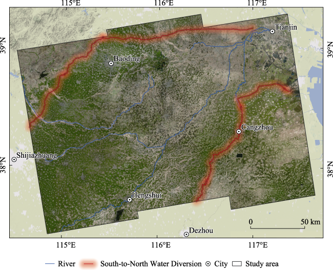
Figure 1 Geographic location of the understudied area in the Hebei Plain
In recent years, the operation of the South-North Water Diversion Project has partially reduced the water supply pressure, and the rate of land subsidence in areas such as Cangzhou in Hebei has noticeably lessened. However, the subsidence in the North China Plain, especially in the Hebei Plain, is generally still in a faster development stage (Guo et al., 2021), and the land subsidence prevention and control situation in the understudied area is still serious. Therefore, the spatial and temporal predictions of land subsidence in the area would be beneficial to early warning and prevention as well as control of the development and distribution of subsidence, which provides a solid reference for social development planning and geologic environmental problem-solving.

2.2 Data preparation

The datasets used in this paper consist of 132 views of Sentinel-1A satellite orbit-raising archived data from May 2017 to November 2021, with detailed parameters presented in Table 1. Based on the Hybrid Pluggable Processing Pipeline (HyP3) service technology provided by Alaska Satellite Facility (ASF), the cloud platform is employed to perform SAR interferometric processing and obtain interferogram collections. Subsequently, the small baseline subset (SBAS) technique is implemented for the inversion and deformation rate estimation of surface deformation time series to generate spatio-temporal series deformation dataset.
Table 1 Radar image information
Radar image Sentinel-1A (S1A)
Flight direction Ascending
Polarization VV+VH
Band C-Band
Beam mode Interferometric wide swath (IW)
Wave length (cm) 5.6
Ground resolution (m) 5×20
Revisit cycle (d) 12
Number of images (scene) 132
Time range 2017.05.20-2021.11.19
As one of the extensively utilized and representative time-series InSAR monitoring techniques, SBAS technology overcomes the effects of spatial and temporal decorrelations of traditional differential interferometry (D-InSAR) technology (Hanssen, 2001; Zebker and Villasenor, 1992), attenuates the limitation of atmospheric effects, and is more suitable for detecting long-term slow deformation, which is more compatible with the development characteristics of land subsidence. The data production process is presented in Figure 2.
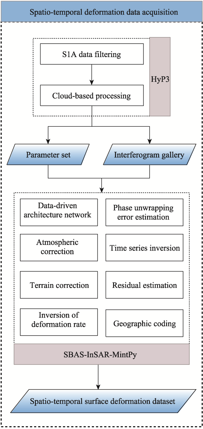
Figure 2 Spatio-temporal subsidence dataset production process
The data obtained in this paper cover an area of about 42,878 km2 and a total of 3,726,515 target points are identified, with a point density of 86 points/km2. The results of previous SAR interference processing experiments reveal that it takes about 7-10 days (including data download and decompression) to process the same data employing a high-performance workstation. However, based on the cloud-based SAR interference service provided by the HyP3, the complete data processing process, including time series inversion, can be completed within hours, substantially enhancing processing efficiency while lessening data storage costs (Arko et al., 2016; Hogenson et al., 2016). With the distributed processing capability of cloud computing, the fast and quasi-real-time acquisition of large-scale and high-precision land subsidence information could be comprehended (Agapiou and Lysandrou, 2020; Nicolau et al., 2021). This issue remarkably improves the lag problem in land subsidence monitoring and thus provides scientific and efficient data support for large-scale surface deformation monitoring, prediction, evolution mechanism, and research works pertinent to prevention and control.
In the present investigation, the predicted distribution of deformation rates in the understudied area is illustrated in Figure 3. The plotted results reveal that the maximum subsidence rate in the data coverage area reaches 165 mm/year during 2017-2021. The spatial variation of land subsidence in the experimentally understudied area is apparent, and several subsidence funnels have been formed, essentially distributed in the central and northeastern parts of the understudied area. Several areas with surface uplift exist, specifically in the southeastern part of the understudied area. Three central areas of subsidence with high deformation rates, high cumulative subsidence, and dense data point distribution, as well as two subsidence edge areas with negative to positive deformation rates and dense data point distribution, are selected for comparison of the future influences of the model prediction.
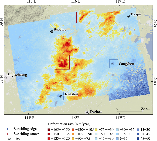
Figure 3 Spatial distribution of land subsidence in the understudied area from 2017 to 2021 (Note: the presented box indicates the typical deformation area.)

3 Methodology

3.1 ConvLSTM

The LSTM structure, also known as the FC-LSTM structure, controls the input and output of each cell unit in the neural network by introducing three gate functions (gates): forgetting gate, input gate, and output gate. The model can establish longer distance temporal dependencies, thereby solving the vanishing gradient problem in traditional RNNs, which is very powerful in dealing with temporal correlation. The specific structure and computational flow of the cells are illustrated in Figure 4a, where several cells are compositely linked to configure the hidden layer structure of the model.
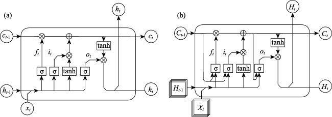
Figure 4 Cells structure of the models: (a) LSTM cells, (b) ConvLSTM cells
The input values of a typical LSTM model include the following three values: (1) the input value of the cell at the current moment xt, (2) the state value of the cell at the previous moment ct-1, (3) the output value of the cell at the previous moment ht-1. The outputs consist of the following two values: (1) the state value of the cell at the current moment ct, (2) the output value of the cell at the current moment ht. The LSTM performs separate gating calculations in the cell. The forgetting gate controls the forgetting of the previous cell state and determines how much of the cell state of the previous moment is retained in the current moment. The input gate controls the accumulation of information and determines how much input is saved to the cell state at the current moment. The output gate controls whether the latest cell state is propagated to the final output and determines how much of the cell state output to the current LSTM output value is. The specific calculation formulas are given in the following:
${{i}_{t}}=\sigma \left( {{W}_{xi}}{{x}_{t}}+{{W}_{h\text{i}}}{{h}_{t-1}}+{{b}_{i}} \right)$
${{f}_{t}}=\sigma \left( {{W}_{xf}}{{x}_{t}}+{{W}_{hf}}{{h}_{t-1}}+{{b}_{f}} \right)$
${{c}_{t}}={{f}_{t}}\circ {{c}_{t-1}}+{{i}_{t}}\circ \tanh \left( {{W}_{xc}}{{x}_{t}}+{{W}_{hc}}{{h}_{t-1}}+{{b}_{c}} \right)$
${{o}_{t}}=\sigma \left( {{W}_{xo}}{{x}_{t}}+{{W}_{ho}}{{h}_{t-1}}+{{b}_{o}} \right)$
${{h}_{t}}={{o}_{t}}\circ \tanh \left( {{c}_{t}} \right)$
where i, f, c, and o denote the input gate, forgetting gate, cell state, and output gate, respectively. In Eqs. (1)–(5), xt represents the input at time t in the time series, and ht denotes the implied state output of the corresponding cell. W is the weight coefficient matrix, b is the bias term, σ is the sigmoid() activation function, tanh is the hyperbolic tangent activation function, and the symbol [$\circ $] denotes the Hadamard product.
Since the LSTM develops a fully connected layer in processing without encoding spatial information, the fully connected structure has too many redundant links, making it difficult for the network to capture the local consistency present in the data during optimization (Shi et al., 2015). In order to consider the spatial dependence of data and better analyze data with spatio-temporal characteristics, Shi et al. (2015) implemented the ConvLSTM neural network. ConvLSTM represents a variant of LSTM, including both convolutional and LSTM networks, which efficiently solves the redundancy problem of the LSTM structure in predicting spatio-temporal data (Li et al., 2020). This approach takes into account both the temporal modeling capability of the LSTM as well as the ability to depict spatial features, and is specifically designed to handle spatio-temporal sequence prediction problems. The cell structure is presented in Figure 4b, and the specific equations for the calculation are as follows:
${{i}_{t}}=\sigma \left( {{W}_{xi}}*{{X}_{t}}+{{W}_{h\text{i}}}*{{H}_{t-1}}+{{W}_{ci}}\circ {{C}_{t-1}}+{{b}_{i}} \right)$
${{f}_{t}}=\sigma \left( {{W}_{xf}}*{{X}_{t}}+{{W}_{hf}}*{{H}_{t-1}}+{{W}_{cf}}\circ {{C}_{t-1}}+{{b}_{f}} \right)$
${{C}_{t}}={{f}_{t}}\circ {{C}_{t-1}}+{{i}_{t}}\circ \tanh \left( {{W}_{xc}}*{{X}_{t}}+{{W}_{hc}}*{{H}_{t-1}}+{{b}_{c}} \right)$
${{o}_{t}}=\sigma \left( {{W}_{xo}}*{{X}_{t}}+{{W}_{ho}}*{{H}_{t-1}}+{{W}_{co}}\circ {{C}_{t}}+{{b}_{o}} \right)$
${{H}_{t}}={{o}_{t}}\circ \tanh \left( {{C}_{t}} \right)$
where [*] denotes the convolutional computation and X, C, H, i, f, and o are all three-dimensional tensors. Comparing Eqs. (1)-(5), we can see that the main difference between ConvLSTM and LSTM is that the connection between the input data and each “gate” by the Hadamard product calculation is replaced with the convolution calculation, as well as the state-to-state calculation. As a result, the features of the center point can be predicted based on the features of the surrounding points in the grid, and the spatial information is preserved as much as possible. Convolution has an appropriate influence on the capture of spatial features. The input data are convolved using kernels to achieve the output as a feature mapping, and one feature mapping can be gained for each kernel, as illustrated in Figure 5. In ConvLSTM, the convolution calculation is accomplished for both the input X and the implied state H, respectively, and then combined with the cell state value C to obtain the H and C at the next moment, and applies the result to process the next X again, and so on, to finally obtain the output results.
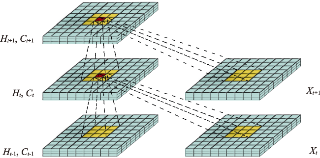
Figure 5 Schematic representation of the convolution calculation of the ConvLSTM
The ConvLSTM layer retains the advantages of the FC-LSTM and uses the “gate” structure to control the data transmission, but replaces each “gate” with a convolution operation instead of the Hadamard product to capture spatial features, which can eliminate numerous spatial redundant features. ConvLSTM divides the weights into two parts for calculation and continuously optimizes the weights through training: one part is contained in the set kernel, which affects the extraction of spatial information through convolution operations; the other part still exists in the cyclic kernel, which realizes the extraction of temporal features with the help of the cyclic kernel, enabling the spatial features to pass through the cycle within the network nodes in the form of 3D tensor, thus enhancing the perception of spatial relationships while ensuring the original ability to capture temporal information.

3.2 Evaluation index

To evaluate the predictive performance of the model, the following evaluation indexes are employed to measure the difference between the accumulated value of the actual and predicted subsidence: Mean square error (MSE), which detects the deviation between the predicted and actual values of the model; Root mean squared error (RMSE), the standard deviation of the fit of the regression system, which avoids the size problem compared to the MSE; Mean absolute error (MAE), which reflects the actual error size, avoids the problem of offsetting errors and presents errors more accurately. These indexes are mathematically expressed by:
$MSE\text{=}\frac{1}{n}\sum\nolimits_{i=1}^{n}{{{\left( \left( {{y}_{i}}-{{{\hat{y}}}_{i}} \right) \right)}^{2}}}$
$RMSE=\sqrt{\frac{1}{n}{{\sum\nolimits_{i=1}^{n}{\left( {{y}_{i}}-{{{\hat{y}}}_{i}} \right)}}^{2}}}$
$MAE=\frac{1}{n}\sum\nolimits_{i=1}^{n}{\left| \left( {{y}_{i}}-{{{\hat{y}}}_{i}} \right) \right|}$
where ${{\hat{y}}_{i}}$ represents the i-th predicted value, yi denotes the i-th observed value, and n is the total number of values. As a general rule, the smaller the value of MAE, RMSE, and MSE, the higher the accuracy of the prediction model.
In order to further evaluate the performance of the model from the visual effect of the output image, this paper aims to use the indexes of human subjective perception: structural similarity (SSIM), and multi-scale SSIM (MS-SSIM) to evaluate the overall structural similarity between the original image and the real one. Generally, the closer the SSIM and MS-SSIM values are to 1, the more similar the two images are. It is understood from the measurement system of SSIM that similarity measurement can be composed of three contrast modules: luminance (l), contrast (c), and structure (s). The calculation formula for each module is provided as follows:
$l(x,y)=\frac{2{{\mu }_{x}}{{\mu }_{y}}+{{C}_{1}}}{\mu _{x}^{2}+\mu _{y}^{2}+{{C}_{1}}}$
$c(x,y)=\frac{2{{\sigma }_{x}}{{\sigma }_{y}}+{{C}_{2}}}{\sigma _{x}^{2}+\sigma _{y}^{2}+{{C}_{2}}}$
$s(x,y)=\frac{{{\sigma }_{xy}}+{{C}_{3}}}{{{\sigma }_{x}}{{\sigma }_{y}}+{{C}_{3}}}$
where μx and μy represent the mean of the original image and predicted image, respectively, $\sigma _{x}^{2}$ and $\sigma _{y}^{2}$ in order the variance of the original image and the predicted image, σxy is the covariance of the original image and the predicted image, and C is a constant whose main functionality is to prevent the divisor from being zero. Based on the above relations, the formulas for the SSIM and MS-SSIM are given as follows:
$SSIM(x,y)={{\left[ l(x,y) \right]}^{\alpha }}{{\left[ c(x,y) \right]}^{\beta }}{{\left[ s(x,y) \right]}^{\gamma }}$
$MSSSIM(x,y)={{\left[ {{l}_{M}}(x,y) \right]}^{\alpha M}}\prod\limits_{j=1}^{M}{{{\left[ {{c}_{j}}(x,y) \right]}^{{{\beta }_{j}}}}}{{\left[ {{s}_{j}}(x,y) \right]}^{{{\gamma }_{j}}}}$
where the factors α, β and γ are employed to adjust the relative importance of the three components in Eqs. (17) and (18). In practice, for the sake of simplicity, the values of these all factors are generally set equal to 1, and ${{C}_{3}}=\frac{{{C}_{2}}}{2}$. The MS-SSIM represents an SSIM index based on the multi-scale (images are scaled according to certain rules, from large to small), where M denotes different scales, incorporating variations in viewing conditions (different resolutions) and thereby providing greater flexibility compared to the SSIM. According to previous experiments (Wang et al., 2003), we set β1=γ1=0.0448, β2=γ2=0.2856, β3=γ3=0.3001, β4=γ4=0.2363, and α5=β5=γ4=0.1333.

4 Experiment

4.1 Model construction and output results

The computer configuration and software environment used in the experiment are as follows: the graphics card is GeForce RTX 2080 Ti; the system is Ubuntu 18.04.1 (64 bit); the program language version is Python 3.8; the integrated development environment is the anaconda. Lastly, the model is designed based on the PyTorch framework.
Due to the large size of the whole image (3589×2809 pixels), inputting the whole frame into the model is bound to take up a lot of GPU memory and affect the processing efficiency. To overcome this dilemma, the input images are cropped and sliced one by one during the experiment. To this end, the low density and insignificant subsidence areas of the target points in the south-western part of the understudied area are safely removed by cropping, and the cropped images (size 3584×2560 pixels) are chunked along the due east and due south directions, respectively. While performing image slicing, an overlap area of around 3% is guaranteed to exist in nearby slices to remove errors caused by zero padding at the edges of the convolution calculation. Finally, the cropped image is divided into 47 slices by 6 rows and 8 columns, each with a size of 512×512 pixels. Subsequently, the dataset is standardized by implementing min-max standardization to generalize the statistical distribution of the uniform sample. The preprocessed dataset is transformed into a tensor format and partitioned into two sets, namely the training set and the testing set, based on a chronological order with a ratio of 8:2. During the training process, the input sequence is randomly shuffled to ensure that the model can generalize well to unseen data. After training, the model outputs the prediction results with the minimum error.
The prediction model is formed by stacking multiple ConvLSTM layers to configure a network structure, and the multiple slice sets obtained from the segmentation are input to the network for training, and the training model for land subsidence prediction is constructed (Figure 6). Since the network applied in this paper has multiple stacked ConvLSTM layers, it exhibits a strong representation capability. Such a property makes it more suitable for making predictions of complex dynamical systems. In the prediction model building experiments, the output results of the validation set are utilized as the basis for comparison, and the parameters of the model are experimented with to find the best one respectively. The number of network layers and the number of neurons are tried from less to more, and the kernel size is tried from small to large, to compare the learning effects of various types of optimizers and finally determine the best model parameters. The whole experimental process is demonstrated in Figure 7, which essentially consists of data pre-processing, neural network training, and neural network prediction.
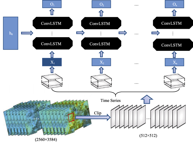
Figure 6 The stacked ConvLSTM prediction model structure
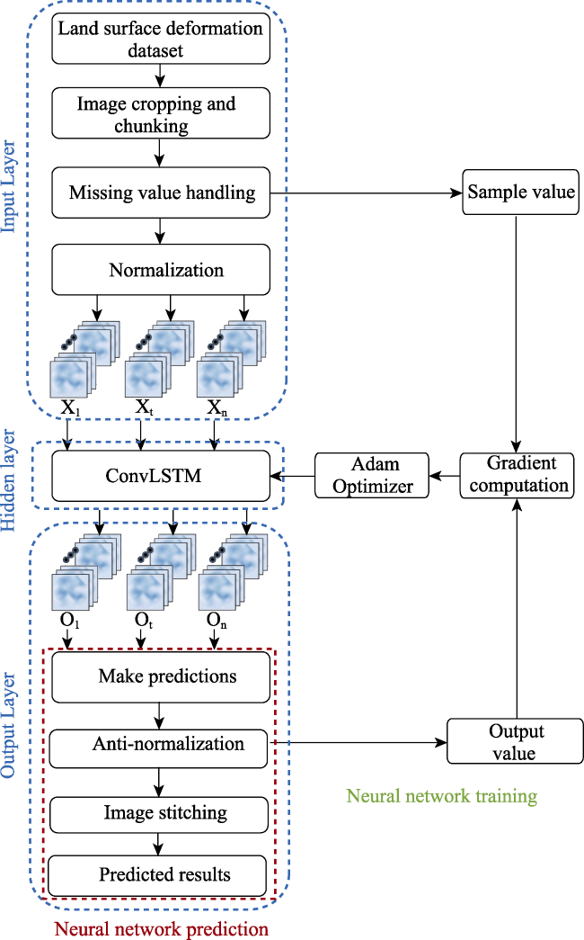
Figure 7 The flowchart of the ConvLSTM network prediction
The essence of model training is to learn the data mapping relationship, and the loss function can measure the gap between the model output and the real data, which is a crucial factor for determining the accuracy of the model. In view of the characteristics of the data itself, MSE may cause the model to fit outliers at the expense of normal sample bias, while MAE is relatively insensitive to outliers and has a more stable gradient. The MSE and MAE are commonly used as loss functions for training respectively, and the loss graphs are plotted for comparison. According to Figure 8a, it is observable that the application of the MAE as the loss function leads to achieving lower loss values. Therefore, the model finally employs the MAE as the loss function and sets the minimum loss function as the optimization objective. Additionally, the model learning rate controls whether the model can accurately find the globally optimal solution, and too large or too small a learning rate will cause the model to settle into the locally optimal solution. We trained using a fixed learning rate of 0.0005, a fixed learning rate of 0.0001, and a variable learning rate with an initial value of 0.001, respectively. In Figure 8b, the corresponding loss curves are plotted to compare the training effect, intercepting the vertical axis range from 0.01 to 0.05. The demonstrated results reveal that the training with a varying learning rate converges faster and the final resulting error of the model is lower. Therefore, the model is finally trained based on the fixed step decay learning rate (StepLR) provided by the scheduler class in PyTorch.
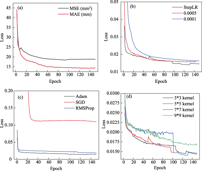
Figure 8 Parameter tuning process curve graph: (a) Loss due to various loss functions, (b) Loss due to various learning rates, (c) Loss due to various optimizers, (d) Loss due to various kernels
In model training, the optimizer can update and compute the network parameters that affect the model output; hence, it can approximate or reach the optimal value, thus minimizing (maximizing) the loss function. In the present paper, the adaptive moment estimation (Adam) algorithm is employed as an optimizer. This approach mixes the advantages of two optimization algorithms, adaptive gradient (AdaGrad) and root mean square propagation (RMSProp) and integrates the first-order and second-order moment estimation of the gradient. Further, the proposed method has the characteristics of less resource consumption and low adjustment requirements and is more suitable for applying to large-scale data prediction (Kingma and Ba, 2017). To validate its advantages, we implement the stochastic gradient descent (SGD) algorithm and RMSProp to compare with Adam. The plotted loss curves for comparison, intercepting the vertical axis range from 0 to 0.2, are given in Figure 8c.
The obtained results demonstrate that the Adam algorithm works better in predicting land subsidence over large areas.
In terms of model structure, the kernel dimension controls the perceptual field size of the model, which straightly affects the information extraction and feature capture performance of the model. We employ 3×3, 5×5, 7×7, and 9×9 kernels for training and the loss curves, intercepting the vertical axis range of 0.013-0.030 (Figure 8d). Comparing their loss curves, it can be seen that the 3×3 and 9×9 kernels produce larger prediction errors, and the 5×5 and 7×7 kernels end up with similar prediction errors, and the curves almost overlap. However, using a larger kernel will increase the time spent on model training, so the model is trained with a 5×5 kernel. After several tests and comparisons, the final structure of the model consists of 3 layers with 32 neurons. Several experimental validations and literature reviews indicate that the errors of single-step prediction are lower than those of multi-step prediction; therefore, the single-step prediction is employed in the present model. The training is terminated by the early stop mechanism, which ends the training after 20 iterations with an accuracy improvement of no more than 0.001, effectively preventing overfitting and reducing the time-consuming inefficient training of the model. Finally, the prediction results of the model are counter-standardized, and the overlapping regions between the cropped image blocks are combined to achieve the final predicted cumulative shape variable atlas after the image stitching is finalized. The model finally outputs a total of 27 views of predicted images from January 11 to November 19, 2021, and the results are demonstrated in Figure 9.
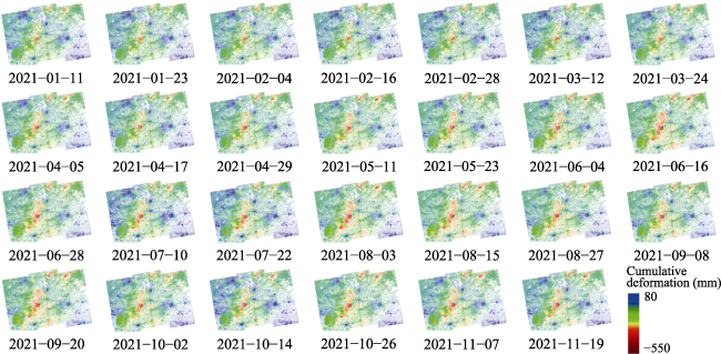
Figure 9 Cumulative shape variable forecast results for the understudied area from January 11, 2021 to November 19, 2021

4.2 Results

4.2.1 Prediction accuracy comparison

The prediction results of the ConvLSTM model and several other machine learning models were evaluated and compared for their predictive accuracy using the MAE, RMSE, and MSE indicators. The prediction results are presented in Table 2. It can be observed from the results provided in this table that the predicted results of the ConvLSTM model are superior to those of other machine learning models, with smaller error indicators in all aspects. The accuracy of the ConvLSTM model's predictions is also significantly improved in comparison with those of the LSTM model. Since the prediction accuracy of other models noticeably differs from that of ConvLSTM, the following comparison is mainly focused on the detailed comparison between the ConvLSTM and LSTM models, to highlight the changes brought by the addition of spatial correlation. In terms of structural similarity, the average SSIM and MS-SSIM of the prediction results based on the ConvLSTM are higher than those of the LSTM, indicating that the prediction results by the ConvLSTM model are more similar to the input images (i.e., the predicted generated images are closer to the actual values). Such a fact clearly proves that the prediction accuracy of the ConvLSTM is more than that of the LSTM.
Table 2 Evaluation of the accuracy of the prediction results
Model MAE (mm) RMSE (mm) MSE (mm2) SSIM MS-SSIM
ARIMA 17.96 24.06 597.62
SVR 16.02 21.31 470.85
RNN 14.61 19.46 393.06
LSTM 11.62 15.61 243.59 0.9518 0.9795
ConvLSTM 10.73 14.31 204.96 0.9654 0.9822
The distribution of the MAE in the prediction period is illustrated in Figure 10. Compared with the previous selection of several subsidence centers with large subsidence rates and dense data points, the ConvLSTM demonstrates better prediction results in the subsidence center area with smaller high values of error and a smaller distribution of high values of error. On the other hand, the LSTM is less effective in predicting the subsidence center region with concentrated high errors and a larger distribution of high errors. Additionally, according to the error pie chart (Figure 11), the ConvLSTM incorporates into a larger proportion of deformation points with fewer errors in the prediction results compared to the LSTM, and the overall predicted MAE by the ConvLSTM in the understudied area is better than that of the LSTM.
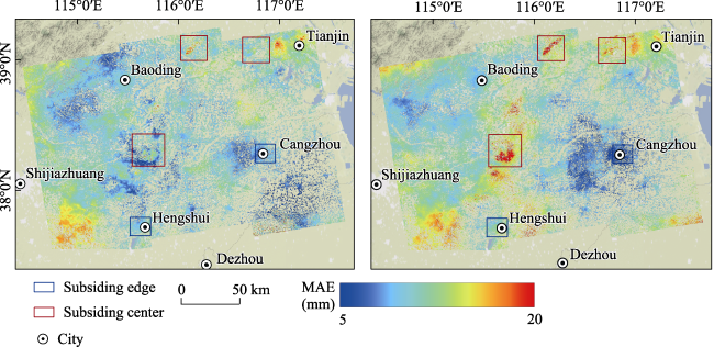
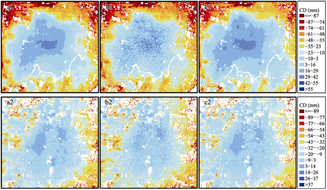
Figure 10 Comparison of MAE distributions between ConvLSTM and LSTM predictions: (a) ConvLSTM, (b) LSTM
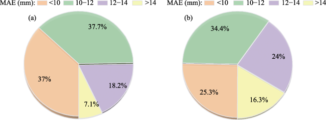
Figure 11 Comparison of MAE proportion differences between ConvLSTM and LSTM predictions: (a) ConvLSTM, (b) LSTM
To more visually compare the error advantages and disadvantages of the two in each part of the understudied area, the MAE difference is further plotted by subtracting the MAE of the predicted results by the ConvLSTM from the MAE of those of the LSTM (the red part exhibits the larger LSTM error and the blue part presents the larger ConvLSTM error) (Figure 12). Statistics analysis reveals that the ConvLSTM model exhibits less prediction error than the LSTM model in about 62.3% of the regions in the understudied area. The difference plot displays that the ConvLSTM remarkably predicts better than LSTM in the area of severe subsidence, and the prediction error in the subsidence center area is noticeably smaller, with a maximum difference of about 21.46 mm from the LSTM prediction results. In other regions with weaker subsidence, the prediction error of the ConvLSTM is slightly larger than that of the LSTM, with a maximum difference of about -19.89 mm from the LSTM prediction. The above results demonstrate that the ConvLSTM exhibits better performance in the overall region in the large-scale land subsidence prediction study, particularly in the prediction of the subsidence center compared with the LSTM.
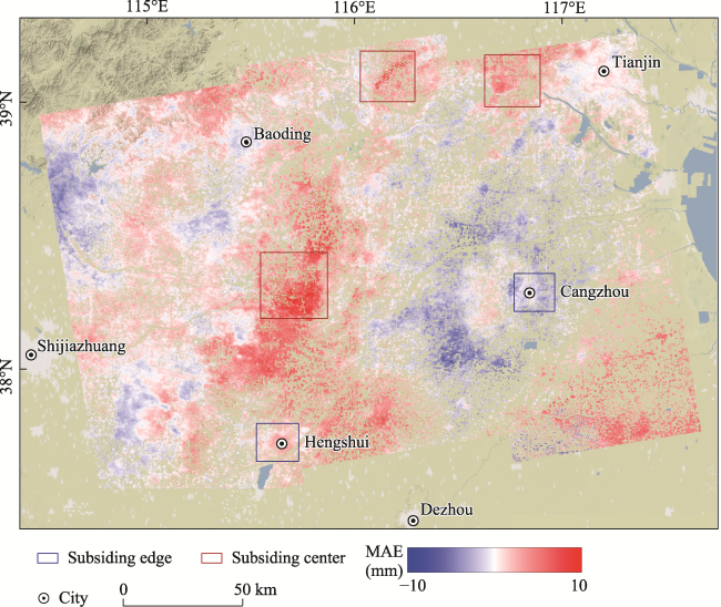
Figure 12 Distribution of MAE differences between ConvLSTM and LSTM prediction results

4.2.2 Spatial distribution comparison

Inherently, regional land subsidence data are closely coupled with spatio-temporal correlations due to the combined influence of multiple natural and anthropogenic factors (Zheng et al., 2014; Lei et al., 2016; Yu et al., 2020), and basically decoupling and decomposition of the spatio-temporal features could lead to ignoring the influence of many potential factors on subsidence. The present model takes the advantage of the convolutional structure in processing spatially correlated lattice data like images and tightly couples it with a recurrent neural network structure to achieve data training and prediction in raster image patterns (Simonyan and Zisserman, 2015; Szegedy et al., 2015).
In order to compare the spatial distribution characteristics of the prediction results, the original data, LSTM prediction results, and ConvLSTM prediction results of the three subsidence center area data for a date image in the prediction cycle are demonstrated in Figure 13. The darker the red in the graph, the greater the cumulative subsidence. A comparison between the three illustrated figures reveals that the prediction results of the ConvLSTM retain the local correlation of surface deformation well due to the extraction of the spatial correlation existing in the surrounding image elements. This issue becomes highlighted in the subsidence center region, which partially preserves the spatial characteristics of the subsidence distribution and is more consistent with the development mechanism of subsidence. In contrast, although the LSTM has a small prediction error in some areas, the adjacent image elements are input as mutually independent points in the model structure, which indicates that the spatial association between adjacent image elements is discarded; therefore, the prediction results obtained by the model are also independent of each other, which is contrary to the first law of geography. Additionally, the prediction results of the ConvLSTM are more accurate than the LSTM in terms of the spatial distribution of subsidence, and the resulting maps are more consistent with the actual subsidence distribution.
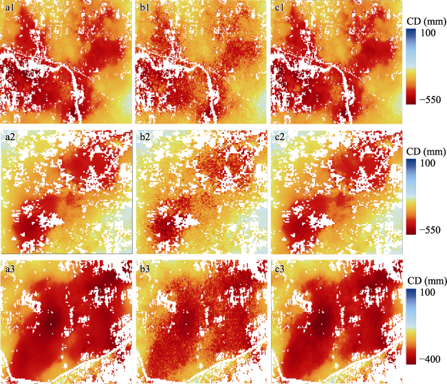
Figure 13 Spatial distribution of cumulative deformation (CD) in the subsidence center: (a) original data, (b) LSTM prediction results, (c) ConvLSTM prediction results
In order to further compare the spatial distribution of the predicted data in the subsidence edge areas, a comparison map was derived based on the distribution of deformation rates in the understudied area by selecting some of the accumulated deformation data in the two subsidence edge areas (i.e., the areas where the surface deformation rates turn from negative to positive). To highlight the deformation boundary, the image is presented as a discrete interpolation, and the minimum value of the accumulated deformation displayed in the image is uniformly set to -100 mm (Figure 14). Through comparing the three figures, although the prediction results of the LSTM are more accurate in terms of predicted values for some weak subsidence areas, the data are dispersed and independent without apparent boundary distinction. In contrast, although the prediction results of the ConvLSTM are not very precise in terms of the distribution area of each deformation value interval, they all preserve the spatial distribution characteristics of the data well and depict clear boundaries of the deformation intervals.
Figure 14 Spatial distribution of cumulative deformation (CD) in the subsidence edge: (a) original data, (b) LSTM prediction results, (c) ConvLSTM prediction results

4.3 Discussion

4.3.1 Analysis of the spatial features

To determine the spatial heterogeneity of the data itself, this paper adopts K-means to perform cluster analysis on the time-series land subsidence data, as a reference to distinguish the distribution of different feature settlement data. Based on the similarity and separability between the time series, the data set is divided into various clusters, which intuitively display the mapping of similar features. Based on the clustering results (Figure 15), it can be observed that although there exists no consistent size relationship between the prediction errors of the ConvLSTM model and the LSTM model in other categories of subsidence data, the prediction errors of ConvLSTM are generally smaller than those of LSTM in class 1, class 2, and class 5 subsidence data. This further demonstrates that spatial correlation does have an impact on the accuracy of prediction results, and the model's predictive performance exhibits noticeable differences in subsidence data with various deformation patterns.
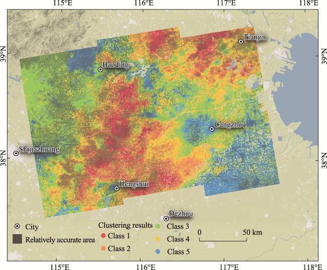
Figure 15 Clustering result of time-series subsidence data features with ConvLSTM prediction error overlay (note: the black areas indicate regions of relatively low prediction error)
According to the multivariate time series (MTS) normalization approach proposed by Providence et al. (2021), the complex external influences of the MTS could be decomposed and generalized into high and low frequencies in time, and global and local in space to refine the various impact components present in the original data. Further, the same dynamical clusters should have some spatial indistinguishability since they share the same local low-frequency components. Consequently, based on the clustering results, this paper selected some adjacent data points in the central subsidence area with smaller prediction errors in ConvLSTM and plotted the autocorrelation relationship of deformation data for comparison (Figure 16).
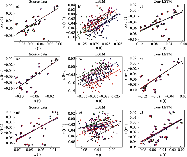
Figure 16 Autocorrelation of adjacent data points at the center of subsidence: (a) original data, (b) LSTM prediction results, (c) ConvLSTM prediction results (note: different colors represent different points of data.)
A further comparison in the predicted results of the ConvLSTM method reveals that the fitted lines of each point in the correlation graph are highly overlapping due to the sharing of the same local low-frequency components. This indicates that this approach effectively preserves the spatial correlation existing among each local data point in the original data and captures the geographical similarity of the land subsidence data in the settlement center region more accurately. However, in the predicted results of the LSTM, the fitted lines of each point in the correlation graph are obviously separated, demonstrating that it has hardly captured the local spatial features of the settlement center region. This also reveals that the independence among data points in the LSTM prediction leads to its deficiency in handling the highly changing data in the settlement center region.
In summary, traditional time-series or hybrid prediction models cannot effectively capture local spatial features, as they operate on input data represented as a vector or scalar and therefore lack the ability to incorporate spatial information. In contrast, the proposed model expands the input and hidden states of the network in the spatial dimension, transforming each time step into a tensor form while preserving the original raster image structure. This approach enables the spatial features to flow in the network nodes as a three-dimensional tensor and ensures that the final output has the same dimension and shape as the prediction target, effectively processing spatio-temporal subsidence data, accurately predicting land subsidence, and outputting subsidence distribution maps. By tightly combining temporal and spatial characteristics, this model overcomes the problem of traditional prediction models' inability to effectively describe spatio-temporal structure. The proposed model provides a solid basis for regional land subsidence prevention and urban development planning, by enabling effective processing of spatio-temporal subsidence data and accurately predicting land subsidence, even in the absence of subsidence drivers data.

4.3.2 Deformation mechanisms and impact on prediction results

Deformation mechanisms play a crucial role in land subsidence. The main deformation mechanisms include groundwater extraction, oil extraction, and natural subsidence due to soil compaction. These mechanisms result in different spatial-temporal patterns of deformation, which in turn impact the prediction performance of different machine learning models. Previous studies have shown that long-term excessive exploitation of groundwater is the main cause of land subsidence in the understudied area (Wang et al., 1994; Liu et al., 2005; Zhang, 2014; Li, 2020). In addition to the temporary land subsidence caused by elastic deformation resulting from the compression of aquifers, which can recover after water pressure is restored, the extensive exploitation of groundwater causes a significant drop in the water table of the aquifer. When the pressure difference between the aquifer and the cohesive soil is sufficient to overcome the interparticle bonding force, water is drained from the cohesive soil, causing pore compression and increasing the contact area between mineral particles, resulting in relative displacement between particles and plastic deformation of the pore structure. When the water pressure in the aquifer is restored, it can only increase the water pressure in the compressed pores of the cohesive soil, but cannot restore the initial porosity and storage capacity of water, leading to permanent land subsidence.
Therefore, there is a positive correlation between the land subsidence and the degree of groundwater level decline in the understudied area. The spatial distribution of the annual subsidence rate is consistent with the distribution of the groundwater level contour lines. In areas with higher subsidence rates, the groundwater level is relatively low, with larger fluctuations in water level amplitude. The distribution of land subsidence is basically consistent with the distribution of the funnel-shaped decline in groundwater level (Figure 17). Due to the spatial variability of the distribution of groundwater level decline funnels, the development of land subsidence also exhibits strong spatial heterogeneity. Not only do different regions have significant differences in their development trends, but the subsidence center region also has strong local features. Through combining with the discussion in Section 4.2.3, ConvLSTM is capable of better capturing the local features of land subsidence by extracting spatial information from the data through its convolutional structure. Therefore, in predicting regions with strong local features (such as subsidence centers), ConvLSTM is expected to produce more precise results than the LSTM-based models that lack spatial information.
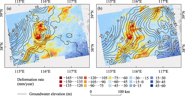
Figure 17 Distribution of groundwater decline funnel and surface settlement in the understudied area (2016): (a) elevation of the shallow groundwater table, (b) elevation of the deep groundwater table
In summary, the deformation mechanisms have a substantial impact on the prediction performance of machine learning models for land subsidence. The ConvLSTM model is more suitable for predicting the land subsidence caused by complex deformation mechanisms, such as groundwater extraction, due to its ability to capture the spatial-temporal patterns of deformation more accurately. ConvLSTM can make relatively accurate land subsidence predictions even without topographic or water level data, which demonstrates that it can alleviate the requirement for complex geological data to a certain extent by capturing the spatial correlation of the data.

5 Conclusions

In the present scrutiny, by constructing a ConvLSTM neural network model, we extend the temporal prediction of subsidence to the spatial dimension, effectively capture the spatial dependence among subsidence data, and achieve a high-precision spatio-temporal prediction of land subsidence taking into account spatial correlation, making up for the drawbacks of traditional machine learning in this area. The test results reveal that the spatio-temporal prediction model of subsidence outperforms the LSTM model of single-point prediction in terms of the MAE and RMSE, and the prediction results are more fundamentally similar to the original data and can remarkably preserve the spatial distribution pattern of subsidence. In the subsidence center region, the ConvLSTM prediction results successfully retain the agglomeration distribution of subsidence. Additionally, in the subsidence edge region, the ConvLSTM prediction results also capture the boundary of the subsidence rate variation better. In view of the complication and substantial regional nature of the causes of land subsidence, the subsidence prediction model based on the ConvLSTM can more rationally consider spatial correlation, combine spatial features with temporal ones, and effectively employ single-factor data for spatio-temporal prediction of the development and distribution of land subsidence, and obtain higher accuracy prediction results in the absence of data on subsidence drivers, providing a solid reference for scientific prevention and control of land subsidence on a large scale.
Generally, this paper validates the applicability of the spatio-temporal prediction in the field of land subsidence prediction and confirms the performance of the ConvLSTM spatio-temporal prediction model in large-scale subsidence prediction. The model still has much room for improvement in prediction accuracy, but due to the wide range of land subsidence and numerous data, it is not appropriate to apply a processing approach with too much computational complexity, and future works are aimed to consider a combination of other data processing approaches with low complexity. Additionally, the present model takes spatial correlation into account, but the interpretability is still moderately weak, and consequently, the need for further research is intensified, particularly linking the model output with physical meaning and constructing comprehensible machine learning spatio-temporal predictors in combination with physical models (Reichstein et al., 2019).
[1]
Agapiou A, Lysandrou V, 2020. Detecting displacements within archaeological sites in Cyprus after a 5.6 magnitude scale earthquake event through the hybrid pluggable processing pipeline (HyP3) cloud-based system and Sentinel-1 Interferometric Synthetic Aperture Radar (InSAR) analysis. IEEE Journal of Selected Topics in Applied Earth Observations and Remote Sensing, 13: 6115-6123.

DOI

[2]
Akbari Asanjan A, Yang T, Hsu K et al., 2018. Short-term precipitation forecast based on the PERSIANN system and LSTM recurrent neural networks. Journal of Geophysical Research: Atmospheres, 123(22): 12, 543-12,563.

[3]
Arko S A, Hogenson R, Geiger A et al., 2016. Sentinel-1 archive and processing in the cloud using the Hybrid Pluggable Processing Pipeline (HyP3) at the ASF DAAC. Presented at the 2016 American Geophysical Union, Fall Meeting, G43A-1040.

[4]
Chen B, Gong H, Chen Y et al., 2020. Land subsidence and its relation with groundwater aquifers in Beijing Plain of China. Science of The Total Environment, 735:139111.

DOI

[5]
Chen M, Tomás R, Li Z et al., 2016. Imaging land subsidence induced by groundwater extraction in Beijing (China) using satellite radar interferometry. Remote Sensing, 8(6): 468. (in Chinese)

DOI

[6]
DeVries P M R, Viégas F, Wattenberg M et al., 2018. Deep learning of aftershock patterns following large earthquakes. Nature, 560(7720): 632-634.

DOI

[7]
Gong H, Li X, Pan Y et al., 2017. Groundwater depletion and regional land subsidence of the Beijing-Tianjin-Hebei area. Bulletin of National Natural Science Foundation of China, 31(1): 72-77. (in Chinese)

[8]
Gong H, Zhang Y, Li X et al., 2009. Research on land subsidence in Beijing based on permanent scatterer radar interferometry. Progress in Natural Science, 19(11): 1261-1266. (in Chinese)

DOI

[9]
Guo H, Li W, Wang L et al., 2021. Present situation and research prospects of the land subsidence driven by groundwater levels in the North China Plain. Hydrogeology & Engineering Geology, 48(3): 162-171. (in Chinese)

[10]
Guo H, Wang L, Chen F et al., 2014. Scientific big data and digital earth. Chinese Science Bulletin, 59(12): 1047-1054. (in Chinese)

[11]
Ham Y G, Kim J H, Luo J J, 2019. Deep learning for multi-year ENSO forecasts. Nature, 573(7775): 568-572.

DOI

[12]
Hanssen R F, 2001. Radar Interferometry: Data Interpretation and Error Analysis (Vol. 2). Springer Science & Business Media.

[13]
Hogenson K, Arko S A, Buechler B et al., 2016. Hybrid Pluggable Processing Pipeline (HyP3): A cloud-based infrastructure for generic processing of SAR data. Presented at the 2016 American Geophysical Union, Fall Meeting, IN21B-1740.

[14]
Huang C J, Kuo P H, 2018. A deep CNN-LSTM model for particulate matter (PM2.5) forecasting in smart cities. Sensors, 18(7): 2220.

DOI

[15]
Kingma D P, Ba J, 2015. Adam: A method for stochastic optimization. International Conference on Learning Representations.

[16]
Lei K, Luo Y, Chen B et al., 2016. Distribution characteristics and influence factors of land subsidence in Beijing area. Geology in China, 43(6): 2216-2228. (in Chinese)

[17]
Li D, Zhang L, Xia G, 2014. Automatic analysis and mining of remote sensing big data. Acta Geodaetica et Cartographica Sinica, 43(12): 1211-1216. (in Chinese)

DOI

[18]
Li H, Zhu L, Dai Z et al., 2021. Spatiotemporal modeling of land subsidence using a geographically weighted deep learning method based on PS-InSAR. Science of The Total Environment, 799: 149244.

DOI

[19]
Li R, 2020. Risk assessment of land subsidence in Hebei Plain[D]. Shijiazhuang: Hebei GEO University. (in Chinese)

[20]
Li W, Tao W, Zhou X et al., 2020. Survey of spatio-temporal sequence prediction methods. Application Research of Computers, 37(10): 2881-2888. (in Chinese)

[21]
Liu B, Wang M, Li Y et al., 2021a. Deep learning for spatio-temporal sequence forecasting: A survey. Journal of Beijing University of Technology, 47(8): 925-941. (in Chinese)

[22]
Liu F, Zhang J, Shen R et al., 2005. Formation mechanism and control measures of land subsidence in Hebei Plain. Journal of Engineering Geology, 13: 16-18. (in Chinese)

[23]
Liu Q, Zhang Y, Deng M et al., 2021b. Time series prediction method of large-scale surface subsidence based on deep learning. Acta Geodaetica et Cartographica Sinica, 50(3): 396-404. (in Chinese)

[24]
Lv Y, Duan Y, Kang W et al., 2015. Traffic flow prediction with big data: A deep learning approach. IEEE Transactions on Intelligent Transportation Systems, 16(2): 865-873.

[25]
Nanni M, Kuijpers B, Körner C et al., 2008. Spatiotemporal data mining. In: Giannotti F, Pedreschi D (eds.). Mobility, Data Mining and Privacy,267-296.

[26]
Nicolau A P, Flores-Anderson A, Griffin R et al., 2021. Assessing SAR C-band data to effectively distinguish modified land uses in a heavily disturbed Amazon forest. International Journal of Applied Earth Observation and Geoinformation, 94: 102214.

DOI

[27]
Pan Y, Pan J, Gong H et al., 2004. Research on the relation between groundwater exploitation and subsidence in Tianjin proper. Geology-Geochemistry, 32(2): 36-39. (in Chinese)

[28]
Pan Z, Li W, 2021. Review of spatio-temporal sequence prediction methods based on deep learning. Journal of Data Acquisition and Processing, 36(6): 436-448. (in Chinese)

[29]
Polson N G, Sokolov V O, 2017. Deep learning for short-term traffic flow prediction. Transportation Research Part C: Emerging Technologies, 79: 1-17.

DOI

[30]
Providence A M, Yang C, Orphe T B et al., 2022. Spatial and temporal normalization for multi-variate time series prediction using machine learning algorithms. Electronics, 11(19): 3167.

DOI

[31]
Reichstein M, Camps-Valls G, Stevens B et al., 2019. Deep learning and process understanding for data-driven Earth system science. Nature, 566(7743): 195-204.

DOI

[32]
Ren L, Zhou G, Dun Z et al., 2018. Case study on suitability and settlement of foundation in goaf site. Rock and Soil Mechanics, 39(8): 2922-2932, 2940. (in Chinese)

[33]
Shearer T R, 1998. A numerical model to calculate land subsidence, applied at Hangu in China. Engineering Geology, 49(2): 85-93.

DOI

[34]
Shi M, Gong H, Chen B et al., 2021. Monitoring of land subsidence in Beijing-Tianjin-Hebei plain during 2016-2018 based on InSAR and Sentinel-1A data. Remote Sensing for Natural Resources, 33(4): 55-63. (in Chinese)

[35]
Shi X, Chen Z, Wang H et al., 2015. Convolutional LSTM network:A machine learning approach for precipitation nowcasting. In: Proceedings of the 28th International Conference on Neural Information Processing Systems - Volume 1 (NIPS’15). Cambridge, MA: MIT Press, 802-810.

[36]
Simonyan K, Zisserman A, 2014. Very deep convolutional networks for large-scale image recognition. Computer Science, arXiv:1409.1556[cs.CV].

[37]
Szegedy C, Liu W, Jia Y et al., 2015. Going deeper with convolutions. 2015 IEEE Conference on Computer Vision and Pattern Recognition (CVPR), MA, USA, 1-9.

[38]
Wang J, Li L, Ge Y et al., 2000. A theoretic framework for spatial analysis. Acta Geographica Sinica, 55(1): 92-103. (in Chinese)

DOI

[39]
Wang L, Guo H, 2015. Effects of continuous drought on groundwater in Beijing plain. Hydrogeology & Engineering Geology, 42(1): 1-6. (in Chinese)

[40]
Wang R, Sun D, Geng S et al., 1994. Dynamics of ground subsidence and its effects on geogeaphical environment in the Tianjin area. Acta Geographica Sinica, 49(4): 317-323. (in Chinese)

DOI

[41]
Wang S, Song X, Wang Q et al., 2009. Shallow groundwater dynamics in North China Plain. Journal of Geographical Sciences, 19(2):175-188.

DOI

[42]
Wang Y, Yang G, 2014. Prediction of composite foundation settlement based on multi-variable gray model. Applied Mechanics and Materials, 580-583: 669-673.

DOI

[43]
Wang Z, Simoncelli E P, Bovik A C, 2003. Multiscale structural similarity for image quality assessment. The Thrity-Seventh Asilomar Conference on Signals, Systems & Computers, 2003, Pacific Grove, CA, USA, 2003: 1398-1402.

[44]
Xu L, Chen N, Chen Z et al., 2021. Spatiotemporal forecasting in earth system science: Methods, uncertainties, predictability and future directions. Earth-Science Reviews, 222: 103828.

DOI

[45]
Yi H, Gao F, 2021. Deformation prediction model of metro based on GA-BP neural network. Journal of Hefei University of Technology (Natural Science), 44(11): 1513-1517. (in Chinese)

[46]
Yu H, Gong H, Chen B et al., 2020. The advance and consideration of land subsidence in Beijing-Tianjin-Hebei region. Science of Surveying and Mapping, 45(4): 125-133, 141. (in Chinese)

[47]
Yue Z, Shen T, Mao X et al., 2020. Study on prediction method of land subsidence based on recurrent neural network. Science of Surveying and Mapping, 45(12): 145-152. (in Chinese)

[48]
Zebker H A, Villasenor J, 1992. Decorrelation in interferometric radar echoes. IEEE Trans. Geosci. Remote Sensing, 30(5): 950-959.

DOI

[49]
Zhai Y, Wang J, Teng Y et al., 2012. Water demand forecasting of Beijing using the time series forecasting method. Journal of Geographical Sciences, 22(5): 919-932.

DOI

[50]
Zhang J, Chu L, Xiao Z et al., 2014. Main progress and achievements of land subsidence survey and monitoring in Hebei Plain. Geological Survey of China, 1(2): 45-50. (in Chinese)

[51]
Zhang J, Zheng Y, Qi D, 2017. Deep spatio-temporal residual networks for citywide crowd flows prediction. Proceedings of the AAAI Conference on Artificial Intelligence, 31(1): arXiv:1610.00081[cs.AI].

[52]
Zhang Q, Chang J, Meng G et al., 2020. Spatio-temporal graph structure learning for traffic forecasting. Proceedings of the AAAI Conference on Artificial Intelligence, 34(1): 1177-1185.

[53]
Zhang Y, 2014. Formation mechanism, monitoring and warning, controlling research of subsidence of Dezhou in North China Plain[D]. Jinan: Shandong University. (in Chinese)

[54]
Zhang Y, Zhang Y, 2013. Land subsidence prediction method of power cables pipe jacking based on the Peck Theory. Advanced Materials Research, 634-638: 3721-3724.

DOI

[55]
Zheng J, Gong H, Li Q et al., 2014. The control factors on subsidence of Beijing plain area in 2003-2009 based on PS-In SAR technology. Bulletin of Surveying and Mapping, 12: 40-43. (in Chinese)

[56]
Zhou C, Gong H, Chen B et al., 2021. Prediction of land subsidence along Tianjin-Baoding high-speed railway using WT-RF method. Remote Sensing for Natural Resources, 33(4): 34-42. (in Chinese)

Outlines

/