Research Articles

Application of modified export coefficient model to estimate nitrogen and phosphorus pollutants from agricultural non-point source

  • ZHAO Xiaoyuan , 1, 4 ,
  • ZHANG Zhongwei 2 ,
  • LIU Xiaojie , 1, 4, * ,
  • ZHANG Qian 1, 4 ,
  • WANG Lingqing 1, 4 ,
  • CHEN Hao 2 ,
  • XIONG Guangcheng 2 ,
  • LIU Yuru 2 ,
  • TANG Qiang 2 ,
  • RUAN Huada Daniel 3
Expand
  • 1. Institute of Geographic Sciences and Natural Resources Research, CAS, Beijing 100101, China
  • 2. Changjiang Institute of Survey, Planning, Design and Research Co., Ltd., Wuhan 430010, China
  • 3. Environmental Science Program, Beijing Normal University-Hong Kong Baptist University United International College, Zhuhai 519080, Guangdong, China
  • 4. College of Resources and Environment, University of Chinese Academy of Sciences, Beijing 100049, China
*Liu Xiaojie (1972-), PhD and Associate Professor, specialized in regional sustainable development. E-mail:

Zhao Xiaoyuan (2000-), Master Candidate, specialized in watershed management. E-mail:

Received date: 2023-02-08

  Accepted date: 2023-06-19

  Online published: 2023-10-08

Supported by

Key Research and Development Program of Hubei Province(2020BCA073)

Independent Innovation Research Program of Changjiang Institute of Survey, Planning, Design and Research Co., Ltd.(CX2019Z05)

Abstract

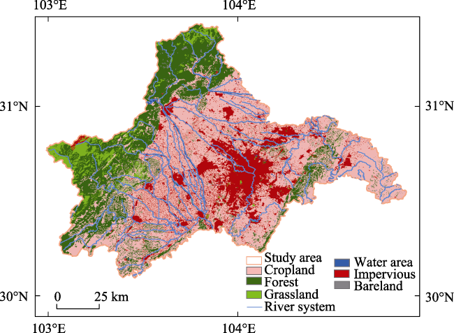
There is a great uncertainty in generation and formation of non-point source (NPS) pollutants, which leads to difficulties in the investigation of monitoring and control. However, accurate calculation of these pollutant loads is closely correlated to control NPS pollutants in agriculture. In addition, the relationships between pollutant load and human activity and physiographic factor remain elusive. In this study, a modified model with the whole process of agricultural NPS pollutant migration was established by introducing factors including rainfall driving, terrain impact, runoff index, leaching index and landscape intercept index for the load calculation. Partial least squares path modeling was applied to explore the interactions between these factors. The simulation results indicated that the average total nitrogen (TN) load intensity was 0.57 t km-2 and the average total phosphorus (TP) load intensity was 0.01 t km-2 in Chengdu Plain. The critical effects identified in this study could provide useful guidance to NPS pollution control. These findings further our understanding of the NPS pollution control in agriculture and the formulation of sustainable preventive measures.

Cite this article

ZHAO Xiaoyuan , ZHANG Zhongwei , LIU Xiaojie , ZHANG Qian , WANG Lingqing , CHEN Hao , XIONG Guangcheng , LIU Yuru , TANG Qiang , RUAN Huada Daniel . Application of modified export coefficient model to estimate nitrogen and phosphorus pollutants from agricultural non-point source[J]. Journal of Geographical Sciences, 2023 , 33(10) : 2094 -2112 . DOI: 10.1007/s11442-023-2167-x

1 Introduction

Non-point source (NPS) pollution is one of the main causes of water pollution in recent years (Guo et al., 2004; Gruber and Galloway, 2008; Wang et al., 2016; Yuan et al., 2021). NPS input, especially agricultural activity, has been a serious aspect of water quality management in China since Stock-breeding Law of the People's Republic of China was issued in 2005. In the Jinjiang River basin, the total nitrogen (TN) load was 12,029.06 t yr-1 and total phosphorous (TP) load was 570.82 t yr-1 (Chen et al., 2013). NPS pollution cannot be ignored their effect on drinking water sources. In the Huangqian Reservoir basin, TN and TP loads were 707.09 t and 114.42 t in 2018, respectively (Hou et al., 2022). In Dongting Lake, TN load was 6.06 t in 2014 (Yuan et al., 2017). As indicated from data summarized above, we can conclude that effect of NPS pollution on freshwater resources is particularly outstanding in China. Large amounts of nitrogen and phosphorus enter aquatic systems causing serious environmental problems such as water eutrophication, oxygen running out, fish and shrimp death and biodiversity decline (Hoppe et al., 2004; Ierodiaconou et al., 2005; Parween et al., 2021; Babaei et al., 2022). For example, eutrophication with reduced river flows contributed to frequency and severity of toxic algae blooms in Australian basins (Young et al., 1996). However, NPS pollution is characterized by randomness of occurrence time, intermittence of occurrence mode, uncertainty of emission path, temporal and spatial variability of pollutant load, and difficulty in simulation and control compared with point source pollution.
Controlling water eutrophication and managing water environment are based on obtaining NPS pollutant loads, so calculating NPS pollutant loads accurately has become important in water research. There are physically based models and empirical models to calculate NPS pollutant loads. The physical models (e.g., Soil and Water Assessment Tool (SWAT), Annualized Agricultural Non-point Source Pollution (AnnAGNPS) and Hydrological Simulation Program Fortran (HSPF)) attempt to simulate the formation of rainfall, runoff and pollutant migration through mathematical models according to the intrinsic mechanism of the NPS pollution formation (Hou and Gao, 2019; Ba et al., 2020). López-Ballesteros et al. (2023) used SWAT to estimate an average TN inflow to the Mar Menor coastal lagoon of 482.4 t yr−1 for 2003-2021. This result is consistent with the range (515±176 t yr−1) obtained by García-Pintado et al. (2007). AnnAGNPS was employed to assess the effectiveness of four best management practices (BMPs) in the Shanmei Reservoir watershed (Chen et al., 2022). Risal et al. (2022) evaluated the performances of SWAT and HSPF in simulating TN and TP load in Big Sunflower River Watershed. The result showed that the HSPF model simulated equally good as SWAT for TN and TP load. In summary, there was consensus that the physical models were widely used in calculation of NPS pollutant loads with accurate results. However, when lots of parameters are not available from the field, they must be determined by calibration instead (Ding, 2010). In contrast, empirical models require less data and have fewer parameters. Export coefficient model (ECM) was established by American scholar in the 1970s and it been gained favor since then because of less required parameters, easy to operate and relative robustness (Mattikalli and Richards, 1996). The ECM was widely applied in many regions of the world (Bowes et al., 2008; Zhang et al., 2019). Based on previous ECM research results, Johnes (1996) proposed a model that considered single source such as land use, livestock quantity and distribution, living emission and treatment level of rural residents and NPS pollutant loads as the sum of a single source of losses.
Some researchers believed that the results of many calculations of NPS pollutant load in China were too high (Ongley et al., 2010). The second national pollution source census bulletin pointed out that chemical oxygen demand (COD), total nitrogen (TN) and total phosphorus (TP) of Chinese agricultural sources accounted for 49.77%, 46.52% and 67.22% of the total pollution source emissions, respectively. According to a report released by the Asian Development Bank, the proportion of COD in rural areas was 1.4 times higher than in urban life source and industrial source, and rural TN and TP loads also accounted for the majority. Since the traditional ECM ignored the underground spatial heterogeneity, temporal and spatial distribution of precipitation and soil conditions, there are some limitations in the model (Noto et al., 2008). Hence, some studies have made modifications to improve ECM. Terrain effect factor and rainfall driving factor were then introduced to analyze the influences of livelihood transformation on NPS pollution (Yuan et al., 2017; Feng et al., 2023a). In the Three Gorges Reservoir region, interception coefficient was added to ECM to calculate the pollutant loads under different land uses (Wang et al., 2015). Cheng et al. (2018) established a modified ECM to calculate the amount of total phosphorus (TP) from agricultural NPS in the Luanhe River Basin of northern China. According to previous studies, the rainfall and terrain factors were mainly considered to the improvement of ECM while some studies considered factors such as surface runoff, landscape interception, but few studies considered the whole process of agricultural NPS pollutant migration.
In recent years, water quality of the upper Yangtze River and its tributaries, Minjiang River, Tuojiang River, have shown obvious seasonal characteristics and an overall trend of deterioration (Hou et al., 2021). Moreover, the Chengdu Plain is part of the upper Yangtze River basin. Meanwhile, the Chengdu Plain is the national important rice, wheat, corn, pig and poultry production base. However, due to the rural population agglomeration, inappropriate use of chemical fertilizers, sewage discharge, poultry and solid waste disposal, which are not effectively treated and recycled, they make the Yangtze River upstream one of the serious NPS polluted areas. Nitrogen and phosphorus lost from agricultural production enter water bodies quickly and are difficult to control, which have a great impact on local and downstream water ecological environment (Feng et al., 2023b; Li et al., 2023). In general, the present study provided new insight with new factors to the modified ECM. The research objectives were (a) to adopt a modified ECM by introducing factors of rainfall driving, terrain impact, runoff index, leaching index and landscape intercept index that can simulate TN load and TP load in Chengdu Plain and (b) to analyze the pollution sources of TN and TP loads and their proportion.

2 Materials and methods

2.1 Study area

The Chengdu Plain is located in southwest China (Figure 1), including Chengdu city and other counties. It is the largest plain in the three provinces (Sichuan, Yunnan and Guizhou) of southwest China. The study area has a warm and humid subtropical Pacific southeast monsoon climate. The average precipitation is approximately 1458 mm and the multi-year average temperature is 16.1°C. June to September is the flood season, accounting for 80% of the total annual rainfall. The western side of Chengdu Plain is the entrance of surface water system, which develops Minjiang River and Tuojiang River (Li et al., 2021). After entering the plain, two rivers diverge in fan shape, confluence at the foot of Longquan Mountain on the east side of the plain.
Figure 1 Location of the Chengdu Plain, southwest China

2.2 Modified export coefficient model

The ECM came from an idea called unit load approach (Johnes, 1996). The model essentially calculated the amount of pollutant load produced in each unit, including human living, livestock husbandry, land use and atmosphere deposition. The formula is outlined as:
$\text{L}=\underset{\text{i}=1}{\overset{\text{n}}{\mathop \sum }}\,{{\text{E}}_{\text{i}}}{{\text{A}}_{\text{i}}}+\text{m}$
where L is the total pollutant load in the study area (kg); Ei is the export coefficient of nutrient pollution source i; Ai is acreage of land use type i in the basin (km2), or the amount of livestock type i and rural population; m is total amount of pollution input by rainfall (kg).
The modified ECM is proposed which considers the effects of hydrometeorology, geography, terrain and human activity on NPS pollution. The formula is shown as the following:
$\text{L}=\underset{\text{i}=1}{\overset{\text{n}}{\mathop \sum }}\,\left[ \text{ }\!\!\alpha\!\!\text{ }\!\!\beta\!\!\text{ }\left( \text{RI} \right)\left( \text{LI} \right)\left( \text{LII} \right) \right]{{\text{E}}_{\text{i}}}{{\text{A}}_{\text{i}}}$
where α is rainfall driving factor; β is terrain impact factor; RI is runoff index; LI is leaching index; LII is landscape intercept index; other indexes are the same as in Eq. (1).

2.2.1 Rainfall driving factor

The calculation formula of rainfall driving factor (α) is consisted of two parts, including the temporal unevenness impact factor (αt), and the spatial unevenness impact factor (αs) (Ding et al., 2010):
$\text{ }\!\!\alpha\!\!\text{ }={{\text{ }\!\!\alpha\!\!\text{ }}_{\text{t}}}\times {{\text{ }\!\!\alpha\!\!\text{ }}_{\text{s}}}=\frac{\text{L}}{{\bar{L}}}\times \frac{{{\text{R}}_{\text{j}}}}{{\bar{R}}}=\frac{\text{f}\left( \text{r} \right)}{\text{f}\left( {\bar{r}} \right)}\times \frac{{{\text{R}}_{\text{j}}}}{{\bar{R}}}$
where L is loss of annual NPS pollutants discharged into water body with the runoff (kg); $\bar{L}$ is average yearly amount of pollutants flowing into water body; Rj is the yearly rainfall in spatial grid unit j of the river basin (mm); $\bar{R}$ is the average yearly rainfall of the whole river basin (mm); f(r) is the relationship between the annual water inflow of agricultural NPS pollutants and the rainfall; $\text{f}\left( {\text{\bar{r}}} \right)$ is loss of nutrients under the multi-year precipitation.
Through regressing analysis, the relationship between the annual water inflow of agricultural NPS pollutants and the precipitation was established according to the rainfall and agricultural pollutant load data in the Minjiang River basin. This study selected total nitrogen (TN) and total phosphorous (TP) to evaluate the agricultural NPS pollution situation. The regression equations are expressed as:
${{L}_{TN}}=10.644r+1312.2\ \ \ \ \left( {{R}^{2}}=0.5811 \right)$
${{L}_{TP}}=3.1521r-24.525\ \ \ \ \left( {{\text{R}}^{2}}=0.5952 \right)$
Based on the precipitation interpolation, the multi-year (from 2016 to 2020) average precipitation in the study area was 1185.98 mm. The Eq. (3) can be described as Eqs. (6) and (7):
${{\alpha }_{TN}}=\frac{10.644r+1312.2}{13935.77}\times \frac{{{R}_{j}}}{{\bar{R}}}$
${{\alpha }_{TP}}=\frac{3.1521r-24.525}{3713.8}\times \frac{{{R}_{j}}}{{\bar{R}}}$

2.2.2 Terrain impact factor

The relationship between the loss of agricultural NPS pollutants and slope is as follows (Aschmann et al., 1999):
$\text{L}=\text{c}{{\text{ }\!\!\theta\!\!\text{ }}^{\text{d}}}$
where L is the yearly water inflow of pollution load (kg); θ is the slope gradient (°).
Based on Eq.(8), the terrain impact factor (β) is shown as follows (Ding et al., 2010):
$\beta=\frac{L\left(\theta_{j}\right)}{L(\bar{\theta})}=\frac{c \theta_{j}^{d}}{c \bar{\theta}^{d}}=\frac{\theta_{j}^{d}}{\bar{\theta}^{d}}$
where θj is the slope for spatial grid unit j of the river basin and $\bar{\theta }$ is the average slope of Chengdu Plain.
The d value is 0.6104 in the Yangtze River (Ding et al., 2010). The average slope is 12.99° in the study area. According to Eq. (9), β can be described using Eq. (10):
$\text{ }\!\!\beta\!\!\text{ }=\frac{\text{ }\!\!\theta\!\!\text{ }_{\text{j}}^{0.6104}}{{{12.99}^{0.6104}}}$

2.2.3 Runoff index

In this study, the SCS-CN flow production model can assess the runoff index (RI) in the Chengdu Plain (Williams and LaSeur, 1976). The runoff volume under different soil types and land uses can be calculated through this method (Auerswald and Haider, 1996):
$Q=\left\{ \begin{matrix} \frac{{{\left( P-0.2S \right)}^{2}}}{P+0.8S},P>0.2\text{S} \\ 0,P\le 0.2S \\ \end{matrix} \right.$
$RI=\frac{Q-{{Q}_{\min }}}{{{Q}_{\max }}-{{Q}_{\min }}}$
where Q is accumulated runoff excess (mm); P is the total rainfall depth which is obtained from field monitoring data in the study area (mm); S is a parameter which is related to the underlying surface.
S is decided by SCS curve number. The parameter is defined as:
$S=\frac{25400}{CN}-254$
$CN=\frac{C{{N}_{2}}}{2.281-0.01281C{{N}_{2}}}$
where CN is a curve parameter that reflects the soil permeability, land use and antecedent soil water conditions. The larger the CN indicates, the smaller the water storage capacity. According to gravel, sand, clay and soil organic matter parameters of the soil, the soil saturated hydraulic conductivity was obtained by using SPAW software, and the hydrological group was conducted to find the corresponding soil type. The CN2 value can be obtained as shown Table S1.
Part of the phosphorus loss is due to soil erosion. Hence, soil erosion needs to be considered in terms of TP runoff index. Universal Soil Loss Equation (USLE) provides a way that evaluates soil loss risk of the Chengdu Plain. The soil erosion amount (A) was defined by Wischmeier et al. (1971). A° is soil erosion factor which is defined as follows:
${A}'=\frac{A-{{A}_{\min }}}{{{A}_{\max }}-{{A}_{\min }}}$
Granular phosphorus accounts for about 90% and dissolved phosphorus accounts for about 10% of the total phosphorus emissions in the Yangtze River. According to this ratio, surface runoff index of TP is described in the following equation:
$R{{I}_{\text{TP}}}=0.1\times RI+0.9\times {A}'$

2.2.4 Leaching index

Soil pollutant such as inorganic nitrogen is easily dissolved in water under natural environment, resulting in its leaching into water system. Therefore, leaching index (LI) was introduced to modified ECM. LI can be determined through precipitation index (PI) and season index (SI). PI characterized the maximum theoretical rainfall can be used for infiltration in the watershed unit. Seasonal changes in rainfall can affect the soil water infiltration, which can be expressed as follows.
$LI=PI\times SI$
$PI=\frac{{{\left( prec-0.4R \right)}^{2}}}{prec+0.6R}$
$SI=\sqrt[\begin{smallmatrix} 3 \\ \end{smallmatrix}]{2\times \frac{prec\left( ls \right)}{prec}}$
$R=\frac{25400}{CN}-254$
where prec is yearly rainfall (mm yr-1); R is yearly soil intercept capacity (mm yr-1); prec(ls) is total rainfall in non-flood season (June-September) (mm); LI needs to be standardized.

2.2.5 Landscape intercept index

Landscape interception is of vital importance in affecting the nutrient pollutant output in a basin. Li et al. (2016) implied landscape intercept index into ECM and proved that the modified model can better explain the NPS pollutant output of different space. Landscape intercept index (LII) is thus established.
$LII=ln\left( \frac{\mathop{\sum }_{DA=1}^{N}{{T}_{D{{A}_{i}}}}}{\tan B} \right)$
where DA is land use type; $\mathop{\sum }^{}{{T}_{DA}}$ is accumulated interception efficiency of forest and grassland; B is slope gradient (°). Interception efficiency of forest and grassland is listed in Table S2, and other land use types are 0. LII needs to be standardized.

2.3 Determination of export coefficients

The agricultural NPS in Chengdu Plain was divided into rural living, livestock and cropland. The export coefficient of rural living was provided by Handbook of Pollutant Discharge Coefficient of Urban Household Sources (The Office of the Leading Group on the First National Census on Pollution Sources, 2008). The export coefficient of livestock was determined based on Handbook of Pollutant Discharge Coefficient of Livestock and Poultry Industry. The export coefficient of cropland was calculated based on Handbook of Fertilizer Loss Coefficient of Agricultural Pollution Sources. The Ei values of modified ECM for rural living, livestock and cropland are listed in Table S3.

2.4 Getis-Ord Gi* Statistic

The Getis-Ord Gi* statistic was applied to analyze the distribution of high value gathering area and low value gathering area of NPS pollutant loads. The calculation method is as follows (Getis and Ord, 1992; Ord and Getis, 1995):
$G_{i}^{*}\left( d \right)=\frac{\mathop{\sum }_{j=1}^{n}{{w}_{ij}}{{x}_{j}}-\bar{X}\mathop{\sum }_{j=1}^{n}{{w}_{ij}}}{S\sqrt{\frac{\left[ n\mathop{\sum }_{j=1}^{n}w_{ij}^{2}-{{\left( \mathop{\sum }_{j=1}^{n}{{w}_{ij}} \right)}^{2}} \right]}{n-1}}}$
$\text{ }\!\!~\!\!\text{ }\bar{X}=\frac{\mathop{\sum }_{j=1}^{\mathrm{n}}{{x}_{j}}}{n}$
$\text{S}=\sqrt{\frac{\mathop{\sum }_{\text{j}=1}^{\text{n}}\text{x}_{\text{j}}^{2}}{\text{n}}-{{\left( {\text{\bar{X}}} \right)}^{2}}}$
where n is the number of regions, i = 1, 2,..., n. wij is a spatial weight matrix between i and j. $\bar{X}$ and S are mean and standard deviation of sample, respectively. When the value of Gi* is positive and significant, the hot spot area appears. When Gi* value is negative and significant, the cold spot area appears.

2.5 Partial least squares path modeling

This study used partial least squares path modeling (PLSPM) to confirm the relationship among NPS pollutant load, modified ECM factors, and human activities. Latent variables consist of four parts, including hydrometeorology features, geomorphic features, land use and human activities. The latent variable hydrometeorology features include rainfall driving factor and runoff index. Terrain impact factor, leaching index and landscape intercept index were considered to represent the latent variable geomorphic features. Land use including paddy field and dry land indicates the latent variable land use. Rural life and livestock breeding were taken to explore the latent variable human activities.
Due to the manifest variable being non-normally distributed, PLSPM was performed to confirm the relationship among NPS pollutant load, modified ECM factors and human activities. Dillon-Goldsteins rho (ρ) and GoF were used to elevate the structural model reliability. The larger the ρ and GoF, the better the structural model robustness.

2.6 Model results verification

Since the modified ECM derived from the original ECM was used in this study, it deserves verifying the robustness of the modified ECM. It is planned to compared the monitoring load data and the simulated load data in Chengdu Plain outlet. The measured data of 2020 were obtained from Hongyuan monitoring section and Yuedianzixia monitoring section. The measured data represent NPS pollution load of the Minjiang (Waijiang) basin. The relative error (Re) was given later in the following section.

2.7 Study data and analysis

The longitude of land use data were 30 m × 30 m, which came from the Resource and Environment Data Center of Chinese Academy of Sciences (https://www.resdc.cn). The source of annual rainfall data were 13 representative rainfall stations in Chengdu Plain form 2016 to 2020 which were obtained from Chengdu Water Authority. The terrain data were processed derived from DEM data. The source of DEM data were obtained from the Computer Network Information Center, Chinese Academy of Sciences (http://www.gscloud.cn). The rural population and livestock were derived from 2020 Chengdu Statistical Yearbook. All the basic data were unified in ArcGIS 10.2 to a resolution of 1 km × 1 km. The rural population and livestock were distributed to rural settlements in land use. The Getis-Ord Gi* (Hot Spot Analysis) was used to analyze spatial agglomeration and correlation of NPS pollution load. The construction of PLSPM was performed using the PLSPM (Sanchez et al., 2017) package with the help of R version 3.6.2 (R Core Team, 2019).

3 Results

3.1 Descriptive statistics and spatial distribution characteristics of factors for modified export coefficient model

Descriptive statistics of factors for modified ECM are listed in Table 1 and Figure 2. The mean values were ranked in the following order: αTPTN>LIITN>LIITP>β>LI>RITN>RITP. Both CV values for β and RITP were over 50%, indicating that these factors varied greatly in Chengdu Plain. The DEM in Chengdu Plain is from 369 to 5277 m (Figure S1) and the spatial distribution characteristics are high in the west and low in the central and eastern parts corresponding to the same trend of CV values for β. The soil erosion amount (A) is from 0 to 8525.58 t km-2 yr-1) in Chengdu Plain (Figure S2), also resulting in high CV values for RITP.
Table 1 Descriptive statistics of factors for modified export coefficient model
Parameter αTN αTP β RITN RITP LI LIITN LIITP
Mean 1.0406 1.0442 0.9020 0.4701 0.1042 0.5215 0.9460 0.9455
Standard deviation 0.3975 0.4141 0.5387 0.2117 0.0971 0.1480 0.1477 0.1481
Coefficient of variation (%) 38.20 39.66 59.72 45.03 93.19 28.38 15.61 15.66
Maximum 2.1651 2.2250 2.8407 1 0.9429 1 1 1
Minimum 0.3363 0.3161 0 0 0 0 0 0
Figure 2 Box plots of factors including rainfall driving factor (α), terrain impact factor (β), runoff index (RI), leaching index (LI)

3.2 Spatial pattern of total nitrogen and total phosphorus pollution risks

TN and TP loads were estimated in Chengdu Plain through modified ECM (Figure 3). The results showed that TN export intensity ranged from 0 to 49.85 t km-2 with a mean value of 0.57 t km-2. TP export intensity ranged from 0 to 2.00 t km-2 with a mean value of 0.01 t km-2. It was obvious that the TN load and TP load intensities exhibited large spatial variation. The region with the highest TN load intensity is located in the west with the highest rainfall and terrain impact factor values, where greater rainfall and gradient contribute to nutrient loss (Wu et al., 2015). In addition, rural population density and cropland area in the high TN load area were larger than in other areas.
Figure 3 The spatial distributions of total nitrogen load (a) and total phosphorus load (b) in the Chengdu Plain
Hot spot analysis was carried out to explore the spatial aggregation features of NPS pollutant loads (Figure 4). The hot spots of TN load were concentrated in Dayi county and Chongzhou city which indicated that these regions had high spatial correlation, and cold spots appeared in the east of Chengdu Plain. The spatial aggregation characteristics of TN load and TP load were roughly the same. According to Chengdu Statistical Yearbook, the gross domestic product of the primary industry in Dayi county and Chongzhou city were at the forefront of Chengdu city, with 340,489 million yuan and 410,848 million yuan, respectively. Moreover, the number of living hogs of Dayi county and Chongzhou city ranked the third and fourth in Chengdu city. Therefore, The NPS pollution brought by aquaculture and agriculture was more serious in Dayi county and Chongzhou city.
Figure 4 The spatial distributions of hot and cold spots of total nitrogen load (a) and total phosphorus load (b). The number in parentheses stands for corresponding confidence

3.3 Source apportionment for agricultural non-point source pollution

The different sources of TN and TP pollution in Chengdu Plain are showed in Figure 5. The estimated TN load from agricultural NPS was 6576.76 t. The contributions to TN load in the Chengdu Plain included livestock husbandry (48.75%), rural living (29.78%), Cropland (21.46%). Obviously, livestock husbandry contributed most and rural living was also a non-negligible source. One important reason was that most of rural wastewater was directly discharged into rivers where sewage collection and treatment were not processed. A considerable part of livestock and poultry breeding bases in the Chengdu Plain were built near the rivers and the manure management measures were not perfect. As a consequence, the wastewater was directly discharged into the rivers. In addition, the long-term storage of livestock and poultry manure also caused nitrate leaching, which was also an important factor affecting the excessive TN standard in the study area.
Figure 5 Total nitrogen and total phosphorus loads from different pollution sources in the Chengdu Plain
The sources contributed to TP load in the Chengdu Plain were found as follows: livestock husbandry 75.54%, rural living 20.61% and cropland 3.85%. Among eight kinds of pollution sources in this area, pig breeding was ranked the largest contributor to TP load (41.50%) that was related to the large number of livestock. For example, there were 2.6 million pigs raised in the study area. In addition, Chengdu Plain is one of the most important farming and animal husbandry areas in China. Frequent and intensive agricultural activities were bound to an increase in NPS pollution.

3.4 Pathways of mediating NPS pollutant loads

PLSPM was used to identify the pathways mediated NPS pollutant loads (Figure 6). For all latent variables of TN and TP, the ρ values were greater than 0.7. The GoF value of TN and TP were 0.514 and 0.601, respectively. The ρ value and GoF index indicated that the measurement and structural models can be used in this study. The hydrometeorology features played a leading role in the direct positive effect of TN load. Geomorphic features had an indirect positive effect on TN load through land use. The indirect negative effect of land use on TN load was greater than the direct positive effect. The path coefficient between human activities and TN load was 0.684, which indicated strongly positive affected on TN load. In terms of PLSPM for TP, hydrometeorology features were one of the factors that directly affect TP load associated with a path coefficient of 0.743. Furthermore, the PLSPM path dia-gram revealed that geomorphic features could indirectly affect TP load by negatively influencing land use. Land use was shown to affect TP load directly and negatively associated with a path coefficient of -0.653.
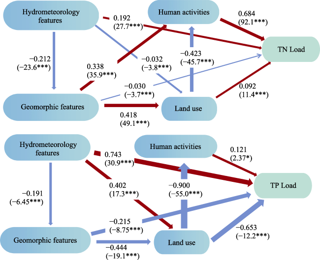
Figure 6 The partial least squares path modeling for the effects of different modified export coefficient model factors on pollutant loads. The red arrows stand for positive effect and blue arrows stand for negative effect. The wider the arrow, the stronger the effect. The number in parentheses represent the t value. * stands for statistical significance at p < 0.05 and *** stands for statistical significance at p < 0.001.

3.5 Robustness of modified export coefficient model

The relative error of TN load in the simulation results was 233.31% of ECM and -16.72% of modified ECM, which was increased by 92.8% in the simulation accuracy (Table 2). The relative error of TP load in the simulation results was 376.73% of ECM and -80.82% of modified ECM, with a 78.5% increase in the simulation accuracy (Table 2). The results revealed that the modified ECM showed more accurate in simulating TN and TP loads than ECM. It also proved that introducing five correction factors to ECM was feasible. The simulation accuracy of TP load was lower than TN load. Some studies have found that ECM is more sensitive in nitrogen load simulation because phosphorus is mostly absorbed by sediment (Wang et al., 2015).
Table 2 Comparison on pollutant loads of simulation accuracy between export coefficient model and modified export coefficient model in Minjiang River watershed (2020)
Pollutant Observation (t) ECM (t) Re (%) Modified ECM (t) Re (%)
Total nitrogen 5053.78 16844.73 233.31 4208.97 -16.72
Total phosphorus 454.47 2166.58 376.73 87.15 -80.82

4 Discussion and conclusions

4.1 Discussion

4.1.1 The relationship between driving factors and pollutant loads

The annual rainfall ranged from 835 to 2209 mm in the study area, which increased from the east to the west (Figure S3). The spatial trend of rainfall driving factor for TN and TP were in accordance with rainfall (Figure S4). The rainfall is a vital factor during NPS pollution happening, such as precipitation intensity, lasting time and spatial heterogeneity. The annual precipitation in the upper reach of Yangtze River was about 850 mm, and rainfall driving factor values were from 0.26 to 3.08 (DN) and from 0.24 to 2.91 (DP) (Ding et al., 2010). The annual average rainfall in Huangqian Reservoir Basin was 721.51 mm, and rainfall driving factor values were from 1.083 to 1.242 (TN) and from 1.216 to 1.393 (TP) (Hou et al., 2022). Topographical heterogeneity can influence the NPS pollution to a large extent and it can be described by terrain impact factor. Slope affects the flow rate of runoff, and ultimately affects the nutrients loss (Li et al., 2006; Shen et al., 2008). The terrain impact factor values ranged from 0 to 2.8407 in the study area, which were in keeping consistence with DEM (Figure S4). Runoff from surface to water system is a significant way controlling the movement of nutrient pollutant (Zhang and Huang, 2011). Some studies about basins over the world had been confirmed that high runoff amount was conducive to soil nitrogen removal followed by entering to water system (Stalnacke et al., 1999; Tomer et al., 2003). Runoff index of TN showed an increasing trend from the west to the east (Figure S4). However, runoff index of TP was not the same as that of TN resulted from soil erosion. P is tightly bound to soil particles in most cases (Caraco and Cole, 2001; Braskerud, 2002). Leaching index ranged from 0 to 1 and most of the study area maintained a large leaching index (Figure S4). Previous studies indicated that nitrate was difficult to be adsorbed by soil and plants due to its negatively charged, and it was easy to infiltration through soil solution (Kiese et al., 2011). The width and slope of vegetation buffer zone can affect the physical retention of P (Uusi-Kämppä et al., 2000). Some other factors such as vegetation area also play a role in physical retention of P (Karr and Schlosser, 1978). However, compared to other factors, vegetated buffer strips width and slope had the greatest impact on retention of P from comprehensively overland flow (Zhang et al., 2010). The larger the width of the interception band and the smaller the slope, the higher the interception efficiency (Syversen, 2005; Ziegler et al., 2006; Roberts et al., 2012). Landscape intercept index showed significant spatial heterogeneity (Figure S4), because different land uses had different interception efficiency including the effect of woodland or grassland being significant (Duchemin and Hogue, 2009).
Compared with other study areas, the Chengdu Plain had relatively lower TN and TP load intensities, e.g. the Fujiang watershed (3.38 t km-2; 0.24 t km-2) (Shen et al., 2011), the Jinjiang River watershed (2.23 t km-2; 0.11 t km-2) (Chen et al., 2013), the Fuji River Catchment (NO3-N load 803 t yr-1; PO4-P load 659 t yr-1) (Delkash et al., 2014), the Redon (TP load 0.25 t km-2) (Pilleboue and Dorioz, 1986). These differences were reasonable because the spatial scales of the above studies were larger than the present study area. In addition, land use types also contributed to these differences. Compared with these previous studies, dry fields were dominant in land uses, whereas the major land use type was paddy field in our study. There were obvious differences between the export coefficient of dry land and paddy field, which the former was significantly larger than the latter (Shen et al., 2011). Another reason was that other factors besides rainfall driving factor and terrain impact factor were involved in modified ECM of this study. These factors demonstrated the whole process by which pollutants enter a water body. Hence, the NPS pollutant loads were lower than those in other study areas.

4.1.2 Contributions of modified export coefficient model factors to non-point source pollution risks

Previous study has reported that human activities including rural life and livestock husbandry have become the important factors of NPS pollution (Follett and Delgado, 2002; Hou et al., 2017). Additionally, the eutrophication level of water in Taihu Lake basin has increased in recent years, which has been resulted from the contribution rate of household wastewater and solid waste to more than 46% of TP load (Liu et al., 2013). Rural life and livestock husbandry were also two main sources for NPS pollution in the Chengdu Plain with a proportion of 78.53% for TN. The lack of sewage and treatment facilities in rural areas of the Chengdu Plain led to NPS pollutants entering the water system through runoff. In addition to the above reason, farmers usually used more than sufficient fertilizers in order to increase crop yields, but this has caused environment pollution. However, fertilizer residues as the N-rich and P-rich pollutants were not effectively managed. It has been indicated that conventional tillage was less available to reduce pollutants in water than no-tillage (Chen et al., 2013).
Geomorphic features have shown negative effect to NPS pollution loads because the slope condition was a key factor for pollutant loss especially the slope below 15° (Figure 6) (Geng et al., 2016). As the slope increases, the area of cropland and vegetation surfaces will be reduced. On the contrary, land cover such as forest and grassland can effectively reduce TN load and TP load. According to Figure 3, TN and TP loads along the river system were larger than other area. Therefore, it is necessary to pay attention to NPS pollution in gentle slope area and restrict agricultural planting and livestock breeding activities along the river (Li et al., 2004; Delgado et al., 2008). As for TN load, the contribution rate of hydrometeorology factor was relatively low, perhaps because the spatial heterogeneity of rainfall was weaker than human activities and other economic factors. However, hydrometeorology factor such as rainfall and runoff could affect soil erosion that directly influenced TP load. As mentioned above, P is usually closely bound to soil particles, which is the reason why the contribution of hydrometeorological factors to TP load is much greater than that to TN load.

4.2 Conclusions

Based on geomorphic features, hydrometeorological characteristics and human activities, modified ECM was developed and integrated to assess TN and TP spatial losses of agricultural NPS and assist NPS pollution control. Rainfall driving factor (α) and terrain impact factor (β) were involved in modified ECM to describe the spatial heterogeneity of rainfall and terrain. Runoff index (RI) simulated the influence of runoff on agricultural NPS pollution. In the process of pollutant migration, groundwater runoff was an important way for the loss of agricultural non-point source pollutants, so leaching index (LI) was introduced. Similarly, vegetation interception cannot be ignored since landscape intercept index (LII) ought to be considered as a factor in modified ECM. Besides, based on the partial least squares path modeling (PLSPM), by considering the impact of regional physical geography, hydrometeorology, human activities and land use, we explored the relationship between pollutant loads and modified ECM factors. The results showed that hydrometeorology factor and human activities were the most critical factors to TP load and TN load, respectively, which should be the focus of agricultural NPS control. The two factors were the initial parameters in ECM and the remaining factors still had an effect on pollutant loads, which were evidence for the rationality of modified ECM. In conclusion, the whole process of agricultural NPS pollutant migration had been considered into this study. Modified ECM can be used to further analyze the characteristics of agricultural NPS pollutant loads in large watersheds, providing a new way to support NPS pollution management.

Supplementary data

A. Supplementary tables

Table S1 CN2 values corresponding to different land uses and soil types
Land use type Soil type
A B C D
Cropland 59 70 78 81
Forest 36 60 73 79
Grassland 76 85 90 93
Water area 100 100 100 100
Impervious land 59 74 82 86
Bareland 60 74 81 85
Table S2 Interception efficiency of forest and grassland to total nitrogen and total phosphorus
Land use type Total nitrogen Total phosphorus
Forest 0.83 0.75
Grassland 0.79 0.70
Table S3 Pollutant export coefficients from agricultural sources
Type Pollution Source Unit Total nitrogen Total phosphorus
Rural living Population kg/(person·a) 5.00 0.45
Livestock Pig kg (head·a) 6.42 1.62
Cattle 37.66 7.44
Sheep 25.94 3.72
Rabbit 0.34 0.05
Chicken 0.34 0.05
Cropland Dry field kg km-2 997.01 55.22
Paddy field 1392.54 11.49

B. Supplementary figures

Figure S1 The spatial distribution of DEM in the Chengdu Plain, southwest China
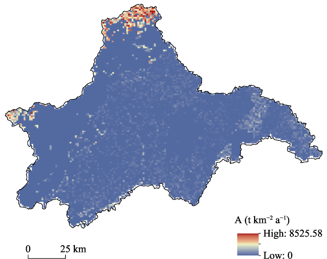
Figure S2 The spatial distribution of soil erosion amount (A) in the Chengdu Plain, southwest China
Figure S3 The spatial distribution of rainfall in the Chengdu Plain, southwest China
Figure S4 The spatial distributions including rainfall driving factor (α), terrain impact factor (β), runoff index (RI), leaching index (LI) and landscape intercept index (LII) in the Chengdu Plain, southwest China
[1]
Aschmann S G, Anderson D P, Croft R J et al., 1999. Using a watershed nutrient dynamics model, WEND, to address watershed-scale nutrient management challenges. Journal of Soil and Water Conservation, 54(4): 630-635.

[2]
Auerswald K, Haider J, 1996. Runoff curve numbers for small grain under German cropping conditions. Journal Environmental Management, 47(3): 223-228.

[3]
Ba W L, Du P F, Liu T et al., 2020. Impacts of climate change and agricultural activities on water quality in the Lower Kaidu River Basin, China. Journal of Geographical Sciences, 30(1): 164-176.

DOI

[4]
Babaei M, Tayemeh M B, Jo M S et al., 2022. Trophic transfer and toxicity of silver nanoparticles along a phytoplankton-zooplankton-fish food chain. Science of The Total Environment, 842: 156807.

DOI

[5]
Bowes M J, Smith J T, Jarvie H P et al., 2008. Modelling of phosphorus inputs to rivers from diffuse and point sources. Science of The Total Environment, 395(2/3): 125-138.

DOI

[6]
Braskerud B C, 2002. Factors affecting nitrogen retention in small constructed wetlands treating agricultural non-point source pollution. Ecological Engineering, 18(3): 351-370.

DOI

[7]
Caraco N F, Cole J J, 2001. Human influence on nitrogen export: A comparison of mesic and xeric catchments. Marine and Freshwater Research, 52(1): 119-125.

DOI

[8]
Chen H Y, Teng Y G, Wang J S, 2013. Load estimation and source apportionment of nonpoint source nitrogen and phosphorus based on integrated application of SLURP model, ECM, and RUSLE: A case study in the Jinjiang River, China. Environmental Monitoring and Assessment, 185: 2009-2021.

DOI PMID

[9]
Chen Y, Lu B B, Xu C Y et al., 2022. Uncertainty evaluation of best management practice effectiveness based on the AnnAGNPS model. Water Resources Management, 36: 1307-1321.

DOI

[10]
Cheng X, Chen L D, Sun R H et al., 2018. An improved export coefficient model to estimate non-point source phosphorus pollution risks under complex precipitation and terrain conditions. Environmental Science and Pollution Research, 25: 20946-20955.

DOI

[11]
Delgado J A, Shaffer M, Hu C et al., 2008. An index approach to assess nitrogen losses to the environment. Ecological Engineering, 32(2): 108-120.

DOI

[12]
Delkash M, Al-Faraj F A M, Scholz M, 2014. Comparing the export coefficient approach with the soil and water assessment tool to predict phosphorous pollution: The Kan watershed case study. Water, Air, & Soil Pollution, 225: 2122.

[13]
Ding X W, 2010. The simulation research on agricultural non-point source pollution in Yongding River in Hebei province. Procedia Environmental Sciences, 2: 1770-1774.

DOI

[14]
Ding X W, Shen Z Y, Hong Q et al., 2010. Development and test of the export coefficient model in the upper reach of the Yangtze River. Journal of Hydrology, 383(3): 233-244.

DOI

[15]
Duchemin M, Hogue R, 2009. Reduction in agricultural non-point source pollution in the first year following establishment of an integrated grass/tree filter strip system in southern Quebec (Canada). Agriculture, Ecosystems & Environment, 131(1/2): 85-97.

DOI

[16]
Feng Z H, Xu C J, Zuo Y P et al., 2023a. Analysis of water quality indexes and their relationships with vegetation using self-organizing map and geographically and temporally weighted regression. Environmental Research, 216: 114587.

DOI

[17]
Feng Z H, Zhang Z W, Zuo Y P et al., 2023b. Analysis of long term water quality variations driven by multiple factors in a typical basin of Beijing-Tianjin-Hebei region combined with neural networks. Journal of Cleaner Production, 382: 135367.

DOI

[18]
Follett R F, Delgado J A, 2002. Nitrogen fate and transport in agricultural systems. Journal of Soil and Water Conservation, 57(6): 402-408.

[19]
García-Pintado J, Martínez-Mena M, Barberá G G et al., 2007. Anthropogenic nutrient sources and loads from a Mediterranean catchment into a coastal lagoon: Mar Menor, Spain. Science of The Total Environment, 373(1): 220-239.

PMID

[20]
Geng R Z, Wang X Y, Pang S J et al., 2016. Identification of key factors and zonation for nonpoint source pollution control in Chaohe River watershed. China Environmental Science, 36(4): 1258-1267. (in Chinese)

[21]
Getis A, Ord J K, 1992. The analysis of spatial association by use of distance statistics. Geographical Analysis, 24(3): 189-206.

DOI

[22]
Gruber N, Galloway J N, 2008. An earth-system perspective of the global nitrogen cycle. Nature, 451: 293-296.

DOI

[23]
Guo H Y, Wang X R, Zhu J G, 2004. Quantification and index of non-point source pollution in Taihu Lake Region with GIS. Environmental Geochemistry and Health, 26: 147-156.

PMID

[24]
Hoppe H, Weilandt M, Orth H, 2004. A combined water management approach based on river water quality standards. Journal of Environmental Informatics, 3(2): 67-76.

DOI

[25]
Hou L, Zhou Z Y, Wang R Y et al., 2022. Research on the non-point source pollution characteristics of important drinking water sources. Water, 14(2): 211.

DOI

[26]
Hou W J, Gao J B, 2019. Simulating runoff generation and its spatial correlation with environmental factors in Sancha River Basin: The southern source of the Wujiang River. Journal of Geographical Sciences, 29(3): 432-448.

DOI

[27]
Hou X N, Xu Z, Tang C H et al., 2021. Spatial distributions of nitrogen and phosphorus losses in a basin and responses to best management practices: Jialing River Basin case study. Agricultural Water Management, 255: 107048.

DOI

[28]
Hou Y, Chen W P, Liao Y H et al., 2017. Modelling of the estimated contributions of different sub-watersheds and sources to phosphorous export and loading from the Dongting Lake watershed, China. Environmental Monitoring and Assessment, 189: 602.

DOI PMID

[29]
Ierodiaconou D, Laurenson L, Leblanc M et al., 2005. The consequences of land use change on nutrient exports: A regional scale assessment south-west Victoria, Australia. Journal of Environmental Management, 74(4): 305-316.

PMID

[30]
Johnes P J, 1996. Evaluation and management of the impact of land use change on the nitrogen and phosphorus load delivered to surface waters: The export coefficient modelling approach. Journal of Hydrology, 183(3/4): 323-349.

DOI

[31]
Karr J R, Schlosser I J, 1978. Water resources and the land-water interface: Water resources in agricultural watersheds can be improved by effective multidisciplinary planning. Science, 201(4352): 229-234.

PMID

[32]
Kiese R, Heinzeller C, Werner C et al., 2011. Quantification of nitrate leaching from German forest ecosystems by use of a process oriented biogeochemical model. Environmental Pollution, 159(11): 3204-3214.

DOI PMID

[33]
Li H P, Liu X M, Huang W Y, 2004. The non-point output of different agriculture landuse types in Zhexi hydraulic region of Taihu Basin. Journal of Geographical Sciences, 14(2): 151-158.

[34]
Li M, Peng J Y, Lu Z X et al., 2023. Research progress on carbon sources and sinks of farmland ecosystems. Resources, Environment and Sustainability, 11: 100099.

DOI

[35]
Li S S, Zhang L, Du Y et al., 2016. Evaluating phosphorus loss for watershed management: Integrating a weighting scheme of watershed heterogeneity into export coefficient model. Environmental Modeling & Assessment, 21: 657-668.

[36]
Li X T, Liang R F, Li Y et al., 2021. Microplastics in inland freshwater environments with different regional functions: A case study on the Chengdu Plain. Science of The Total Environment, 789: 147938.

DOI

[37]
Li Y, Wang C, Tang H L, 2006. Research advances in nutrient runoff on sloping land in watersheds. Aquatic Ecosystem Health & Management, 9(1): 27-32.

[38]
Liu B B, Liu H, Zhang B et al., 2013. Modeling nutrient release in the Tai Lake Basin of China: Source identification and policy implications. Environmental Management, 51: 724-737.

DOI PMID

[39]
López-Ballesteros A, Trolle D, Srinivasan R et al., 2023. Assessing the effectiveness of potential best management practices for science-informed decision support at the watershed scale: The case of the Mar Menor coastal lagoon, Spain. Science of The Total Environment, 859: 160114.

[40]
Mattikalli N M, Richards K S, 1996. Estimation of surface water quality changes in response to land use change: Application of the export coefficient model using remote sensing and geographical information system. Journal of Environmental Management, 48(3): 263-282.

DOI

[41]
Noto L V, Ivanov V Y, Bras R L et al., 2008. Effects of initialization on response of a fully-distributed hydrologic model. Journal of Hydrology, 352(1/2): 107-125.

DOI

[42]
Ongley E D, Zhang X L, Yu T, 2010. Current status of agricultural and rural non-point source pollution assessment in China. Environmental Pollution, 158(5): 1159-1168.

DOI PMID

[43]
Ord J K, Getis A, 1995. Local spatial autocorrelation statistics: Distributional issues and an application. Geographical Analysis, 27(4): 286-306.

DOI

[44]
Parween M, Ramanathan A L, Raju N J, 2021. Assessment of toxicity and potential health risk from persistent pesticides and heavy metals along the Delhi stretch of river Yamuna. Environmental Research, 202: 111780.

DOI

[45]
Pilleboue E, Dorioz J M, 1986. Mass-balance and transfer mechanisms of phosphorus in a rural watershed of Lac Leman, France. Sediments and Water Interactions, 9: 99-102.

[46]
R Core Team, 2019. R: a language and environment for statistical computing. R Foundation for Statistical Computing, Vienna, Austria. https://www.R-project.org/.

[47]
Risal A, Parajuli P B, Ouyang Y, 2022. Impact of BMPs on water quality: A case study in Big Sunflower River watershed, Mississippi. International Journal of River Basin Management, 20(3): 375-388.

DOI

[48]
Roberts W M, Stutter M I, Haygarth P M, 2012. Phosphorus retention and remobilization in vegetated buffer strips: A review. Journal of Environmental Quality, 41(2): 389-399.

DOI PMID

[49]
Sanchez G, Trinchera L, Russolillo G, 2017. plspm: tools for partial least squares path modeling (PLS-PM). R package version 0.4.9. https://CRAN.R-project.org/package=plspm.

[50]
Shen Z Y, Hong Q H, Chu Z et al., 2011. A framework for priority non-point source area identification and load estimation integrated with APPI and PLOAD model in Fujiang Watershed, China. Agricultural Water Management, 98(6): 977-989.

DOI

[51]
Shen Z Y, Hong Q, Yu H et al., 2008. Parameter uncertainty analysis of the non-point source pollution in the Daning River watershed of the Three Gorges Reservoir Region, China. Science of The Total Environment, 405(1-3): 195-205.

DOI PMID

[52]
Stalnacke P, Grimvall A, Sundblad K et al., 1999. Estimation of riverine loads of nitrogen and phosphorus to the Baltic Sea, 1970-1993. Environmental Monitoring and Assessment, 58: 173-200.

DOI

[53]
Syversen N, 2005. Effect and design of buffer zones in the Nordic climate: The influence of width, amount of surface runoff, seasonal variation and vegetation type on retention efficiency for nutrient and particle runoff. Ecological Engineering, 24(5): 483-490.

DOI

[54]
The Office of the Leading Group on the First National Census on Pollution Sources, 2008. Handbook on the First National Census on Pollution Sources. Report, China's State Council, Beijing.

[55]
Tomer M D, Meek D W, Jaynes D B et al., 2003. Evaluation of nitrate nitrogen fluxes from a tile-drained watershed in central Iowa. Journal of Environmental Quality, 32(2): 642-653.

PMID

[56]
Uusi-Kämppä J, Braskerud B, Jansson H et al., 2000. Buffer zones and constructed wetlands as filters for agricultural phosphorus. Journal of Environmental Quality, 29(1): 151-158.

[57]
Wang J L, Shao J A, Wang D et al., 2015. Simulation of the dissolved nitrogen and phosphorus loads in different land uses in the Three Gorges Reservoir region: Based on the improved export coefficient model. Environmental Science: Processes & Impacts, 17(11): 1976-1989.

[58]
Wang J L, Shao J A, Wang D et al., 2016. Identification of the “source” and “sink” patterns influencing non-point source pollution in the Three Gorges Reservoir area. Journal of Geographical Sciences, 26(10): 1431-1448.

DOI

[59]
Williams J R, LaSeur W V, 1976. Water yield model using SCS curve numbers. Journal of the Hydraulics Division, 102(9): 1241-1253.

DOI

[60]
Wischmeier W H, Johnson C B, Cross B, 1971. Soil erodibility nomograph for farmland and construction sites. Journal of Soil and Water Conservation, 26(5): 189-193.

[61]
Wu L, Gao J E, Ma X Y et al., 2015. Application of modified export coefficient method on the load estimation of non-point source nitrogen and phosphorus pollution of soil and water loss in semiarid regions. Environmental Science and Pollution Research, 22: 10647-10660.

DOI

[62]
Young W J, Marston F M, Davis R J, 1996. Nutrient export and land use in Australian catchments. Journal of Environmental Management, 47(2): 165-183.

DOI

[63]
Yuan C C, Liu L M, Ye J W et al., 2017. Assessing the effects of rural livelihood transition on non-point source pollution: A coupled ABM-IECM model. Environmental Science and Pollution Research, 24(14): 12899-12917.

DOI

[64]
Yuan Z W, Pang Y J, Gao J Q et al., 2021. Improving quantification of rainfall runoff pollutant loads with consideration of path curb and field ridge. Resources, Environment and Sustainability, 6: 100042.

DOI

[65]
Zhang H, Huang G H, 2011. Assessment of non-point source pollution using a spatial multicriteria analysis approach. Ecological Modelling, 222(2): 313-321.

DOI

[66]
Zhang L G, Wang Z Q, Chai J et al., 2019. Temporal and spatial changes of non-point source N and P and its decoupling from agricultural development in water source area of middle route of the south-to-north water diversion project. Sustainability, 11(3): 895.

DOI

[67]
Zhang X Y, Liu X M, Zhang M H et al., 2010. A review of vegetated buffers and a meta-analysis of their mitigation efficacy in reducing nonpoint source pollution. Journal of Environmental Quality, 39(1): 76-84.

DOI PMID

[68]
Ziegler A D, Tran L T, Giambelluca T W et al., 2006. Effective slope lengths for buffering hillslope surface runoff in fragmented landscapes in northern Vietnam. Forest Ecology and Management, 224(1/2): 104-118.

DOI

Outlines

/