Research Articles

Measuring glacier changes in the Tianshan Mountains over the past 20 years using Google Earth Engine and machine learning

  • ZHUANG Lichao , 1, 2, 3 ,
  • KE Changqing , 1, 2, 3, * ,
  • CAI Yu 1, 2, 3 ,
  • NOURANI Vahid 4
Expand
  • 1. Jiangsu Provincial Key Laboratory of Geographic Information Science and Technology, Key Laboratory for Land Satellite Remote Sensing Applications of Ministry of Natural Resources, School of Geography and Ocean Science, Nanjing University, Nanjing 210023, China
  • 2. Collaborative Innovation Center of Novel Software Technology and Industrialization, Nanjing 210023, China
  • 3. Collaborative Innovation Center of South China Sea Studies, Nanjing 210023, China
  • 4. Center of Excellence in Hydroinformatics, Faculty of Civil Engineering, University of Tabriz, Tabriz, Iran
*Ke Changqing, Professor, specialized in cryosphere remote sensing. E-mail:

Zhuang Lichao, PhD Candidate, specialized in cryosphere remote sensing. E-mail:

Received date: 2022-11-10

  Accepted date: 2023-05-09

  Online published: 2023-10-08

Supported by

National Natural Science Foundation of China(41830105)

National Natural Science Foundation of China(42011530120)

Abstract

Glaciers in the Tianshan Mountains are an essential water resource in Central Asia, and it is necessary to identify their variations at large spatial scales with high resolution. We combined optical and SAR images, based on several machine learning algorithms and ERA-5 land data provided by Google Earth Engine, to map and explore the glacier distribution and changes in the Tianshan in 2001, 2011, and 2021. Random forest was the best performing classifier, and the overall glacier area retreat rate showed acceleration from 0.87%/a to 1.49%/a, while among the sub-regions, Dzhungarsky Alatau, Central and Northern/Western Tianshan, and Eastern Tianshan showed a slower, stable, and sharp increase rates after 2011, respectively. Glacier retreat was more severe in the mountain periphery, low plains and valleys, with more area lost near the glacier equilibrium line. The sustained increase in summer temperatures was the primary driver of accelerated glacier retreat. Our work demonstrates the advantage and reliability of fusing multisource images to map glacier distributions with high spatial and temporal resolutions using Google Earth Engine. Its high recognition accuracy helped to conduct more accurate and time-continuous glacier change studies for the study area.

Cite this article

ZHUANG Lichao , KE Changqing , CAI Yu , NOURANI Vahid . Measuring glacier changes in the Tianshan Mountains over the past 20 years using Google Earth Engine and machine learning[J]. Journal of Geographical Sciences, 2023 , 33(9) : 1939 -1964 . DOI: 10.1007/s11442-023-2160-4

1 Introduction

The global glacier retreat at the beginning of the 21st century has been unprecedented compared to the past 2000 years (medium confidence), and different projection scenarios indicate that this retreat will continue in the future (Masson-Delmotte et al., 2021). The Tianshan, known as the ‘water towers of Central Asia,’ are located in the hinterland of Eurasia, are far from the ocean, and play an essential role in the regional climate system, with meltwater from the mountains being an important source of water resources for the semiarid and arid regions where they are located (Chen et al., 2016; Pritchard 2019). In the context of global warming, warming trends have been particularly evident in the Tianshan (Ji et al., 2014), and glaciers and snowpack in the region are subjected to multiple effects of temperature and precipitation changes, which in turn have implications for water use by the region’s population (Sorg et al., 2012; Miles et al., 2021). Similar to global trends, the Tianshan glaciers have shown a continuous retreat over the past decades (Farinotti et al., 2015; Milner et al., 2017; Sommer et al., 2020), which will impose some limitations on long-term freshwater resource use in Central Asia (Huss and Hock, 2018; Rounce et al., 2020). Studies have also shown the shrinkage of glacier area and the acceleration of glacier area retreat in the Tianshan after 2011 (Hagg et al., 2013; Petrakov et al., 2016). In contrast, current studies on glacier changes in the Tianshan have focused mainly on some small-scale areas (Kraaijenbrink et al., 2017; Zhang et al., 2019c; Liu et al., 2020; Cai et al., 2021; Zhang et al., 2022a), with a coarse resolution in the estimation of changes on a larger scale (Deng and Chen 2017; Bhattacharya et al., 2021); however, more detailed reports on the spatial variability of glacier changes across the Tianshan are still lacking.
Machine learning-based classification methods have been applied to measure glacier changes (Huang et al., 2011; Xie et al., 2020; Yousuf et al., 2020), and these methods can effectively improve the accuracy of identifying features on the glaciers and surrounding surfaces (Maxwell et al., 2018). However, machine learning requires a large amount of remote sensing data with a high spatial and temporal resolution for mining adequate information, which places high demands on data storage, computing, and analysis. As a result, some geospatial cloud computing platforms, such as Google Earth Engine (GEE), have emerged gradually in recent years. Many researchers use the GEE platform for its convenient and mature linkage with Google Cloud, its wide range of collection and integration of mainstream remote sensing data, and its easy-to-use operation (Gorelick et al., 2017; Tamiminia et al., 2020). GEE can rapidly process massive amounts of data at the pixel scale in the cloud and derive computational results, and it has been introduced to support cutting-edge remote sensing research in glaciated environmental change (Bevington and Menounos 2022).
This work aimed to develop an automatic algorithm to identify glaciers in the Tianshan and map their spatiotemporal portal distribution to explore the change process of supraglacial debris cover, clean ice, and snow by combining glacier inventory data and remotely sensed images on the GEE geospatial analysis platform. Principal component analysis (PCA) was utilized to filter the variables with the highest correlation, and four machine learning algorithms, random forest (RF), support vector machine (SVM), gradient tree boost (GTB), and classification and regression tree (CART), were used to classify supra-glacial features, including debris-covered ice, at the pixel level. Raw spectral information, band ratios from multi-temporal satellite imagery, and topographical components derived from digital elevation models (DEM) and digital surface models (DSM) were extracted as feature variables via the machine learning algorithms. The same scheme was used to generate a decadal interval series of glacier areas in the study area for 2001, 2011 and 2021. Finally, the results were comprehensively analysed, including recognition accuracy and rate of change, and discussed with relevant topographic and climatic data. This study combined PCA results from optical and SAR data based on machine learning algorithms on GEE for glacier classification and obtained high accuracy.

2 Study area

The Tianshan Mountains (Figure 1, hereafter Tianshan), one of the seven major mountain ranges in the world, are located in the central region of Eurasia; the mountain range has an average altitude of approximately 4000 m a.s.l. and extends across China, Kazakhstan, Kyrgyzstan, and Uzbekistan (Chen et al., 2016). The Tianshan is approximately 2500 km long from east to west and 250 to 350 km wide from north to south, and the maximum width of the mountain system is approximately 800 km (Zhang et al., 2022b). It is the largest independent zonal mountain range, the farthest from the sea, and the most prominent mountain system in arid regions globally. Situated in the middle temperate zone with a mountainous continental climate, the Tianshan Range has an obvious vertical zonality (Zhou et al., 2021). The annual precipitation in high-elevation areas can reach 400-800 mm, creating climatic conditions that are very conducive to the formation and development of glaciers and permafrost in the Tianshan, whereas the annual precipitation at low elevations is approximately 100-200 mm (Chen et al., 2016). The Tianshan played a pivotal role in people’s lives owing to their abundant water, mineral, plant, and animal resources. Known as the ‘Water Tower of Central Asia,’ glaciers in the Tianshan are the most precious natural freshwater resource.
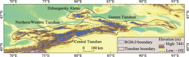
Figure 1 Location of the Tianshan Mountains. The blue line is the glacial boundary at Randolph Glacier Inventory V6.0, the black line is the extent of the Tianshan, and the dotted line denotes the glacial-climate sub-regions. These delineations of glacial-climate sub-regions were produced by the Hindu Kush Himalaya Monitoring and Assessment Program or HiMAP.
According to the latest Randolph Glacier Inventory V6.0, or RGI6.0 (RGI Consortium 2017), 13,998 glaciers exist in the Tianshan, with a total area of 11,864 km2. Among them, seven glaciers cover areas greater than 100 km2, with a total area of 1602.39 km2, accounting for 0.05% and 13.5% of the total number and area of glaciers in the Tianshan, respectively. The South Inylchek Glacier in north-eastern Kyrgyzstan is the largest in the Tianshan, covering an area of 373.92 km2.

3 Materials and methods

3.1 Data

Landsat 5/7 images from 2001 and Landsat 5 images from 2011 were obtained from the GEE platform to extract the glaciers in the Tianshan in 2001 and 2011. In 2021, Landsat 8 was utilized to supplement the validation process by filling in missing pixels for certain Sentinel 2 pixels where cloud interference could not be eliminated. These orthorectified images represent the surface reflectance values calculated using the Landsat Ecosystem Disturbance Adaptive Processing System (LEDAPS) algorithm for Landsat 5 and 7 (Masek et al., 2006), and they have a spatial resolution of 30 m.
Sentinel-1 contains all of the ground range detected (GRD) scenes. Each scene has four band combinations (corresponding to scene polarization), and the possible combinations are single-band VV or HH and dual-band VV+VH or HH+HV. Sentinel-2 is a wide-swath, high-resolution, multispectral imaging mission supporting Copernicus Land Monitoring studies. The Sentinel-2 L2 data on GEE were downloaded from scihub and were computed by running sen2cor. Sentinel series data that had a spatial resolution of 10 m were used for glacier classification in 2020, and some data from 2021 were used to replace missing 2020 data.
The global 25 m PALSAR/PALSAR-2 (The Phased Array type L-band Synthetic Aperture Radar) mosaic is a seamless global SAR image created by mosaicking strips of SAR imagery from PALSAR/PALSAR-2. For each year and location, the strip data were selected through visual inspection of the browse mosaics available over the period, with those showing a minimum response to surface moisture were preferentially used. Its polarization backscattering coefficient contains HH and HV, and this dataset was used as the SAR data source for 2011.
Two sources of digital elevation and surface data were used: NASADEM and ALOS World 3D-30 m (AW3D30). NASADEM reprocesses SRTM data with improved accuracy by incorporating auxiliary data. AW3D30 is a global DSM dataset with a horizontal resolution of approximately 30 m (1 arcsec mesh). The DEM data used to extract ridge lines and calculate glacier length were AW3D30, and the DEMs used to calculate the surface elevations, slopes, and aspects of glaciers were NASADEM and AW3D30.
The Randolph Glacier Inventory (RGI 2.0 and 6.0, representing the glacier boundaries before 2000 and in approximately 2010, respectively) was applied as a reference to evaluate the glacier delineation results. RGI glacier outlines and a distance-based buffer of 100 m were used as the baseline representation of glacier area in this study. Some glaciers were missed in version 6.0, so they were supplemented with version 2.0. The glacier inventory was uploaded to the GEE Assets.
To analyse regional climate forcing, the ERA5-Land Monthly Averaged by Hour of Day reanalysis data was analysed to investigate changes in climate throughout the study. The monthly 2-m air temperature and total monthly precipitation from 1991 to 2021 were considered, and this Climate Reanalysis dataset had a horizontal resolution of 0.1°× 0.1° (the resolution on GEE platform is marked as 11,132 m).
The names of the datasets used on the GEE and their respective time scales, quantities, and resolutions can be found in Table 1.
Table 1 The datasets employed in this study, along with their respective time ranges, quantities, resolutions, and names on GEE
Data source Time ranges Quantity Resolution Names on GEE
Landsat 5 2001.05.01-2001.10.31 142 30 m LANDSAT/LT05/C01/T1_TOA
Landsat 7 2001.05.01-2001.10.31 250 30 m LANDSAT/LE07/C01/T1_TOA
Landsat 5 2011.05.01-2011.10.31 413 30 m LANDSAT/LT05/C01/T1_TOA
Landsat 8 2021.05.01-2021.10.31 629 30 m LANDSAT/LC08/C01/T1_TOA
PALSAR/PALSAR-2 2008-2010 3 25 m JAXA/ALOS/PALSAR/YEARLY/SAR
Sentinel-1 2021.05.01-2021.10.31 1038 10 m COPERNICUS/S1_GRD
Sentinel-2 2021.05.01-2021.10.31 6709 10 m COPERNICUS/S2
NASADEM 30 m NASA/NASADEM_HGT/001
ALOS DSM 2006-2011 90 30 m JAXA/ALOS/AW3D30/V3_2
ERA5_LAND 1991-2021 271,752 11,132 m ECMWF/ERA5_LAND/HOURLY

3.2 Methods

A pixel-based machine learning classification method was used to identify and classify ice, snow, debris-covered ice and other features (water, land, vegetation, etc.) on GEE, and the whole process consisted of several significant processing steps (Figure 2). First, satellite images of selected years were filtered, and annual image composites were generated after masking clouds and cloud shadows. Second, manual visual interpretation was performed based on the annual image composites from the previous step to select feature sample points and generate training and validation datasets. Third, multiple indices were generated from the multi-sensor data and fused into the original image in the form of multiple bands together with elevation and slope data. PCA compressed many bands in the original image into fewer uncorrelated bands. The first three significant bands which could explains 95% of the overall variance were selected as the input data for the subsequent supervised classification. Fourth, four machine learning algorithms (RF, SVM, GTB, CART) were applied and evalu- ated and the one with the highest accuracy was selected. The study area was divided into 0.5°×0.5° geographic grid cells, and the classifier was trained to extract glaciers and other features based on the classification features of the training dataset. Fifth, the classification results were post-processed to eliminate the ‘salt-and-pepper noise’, and the results were compared with the validation dataset to evaluate the classification accuracy. Sixth, the changes in glacier areas were analysed and the influence of climatic and topographic factors were explored.
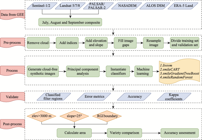
Figure 2 Flowchart for the classification of glacier surface features using machine learning algorithms on the GEE platform

3.2.1 Imagery preprocessing, machine learning, and postprocessing based on GEE

Three years (2001, 2011, and 2021) were selected for identifying glaciers and generating contours based on the classification results. For 2001, the datasets used were Landsat 7 and NASADEM, while Landsat 5, PALSAR/PALSAR-2, and ALOS DSM were used for 2011, and three datasets, Sentinel-1, Sentinel-2, and ALOS DSM, were used for glacier identification in 2021. The screening time of the datasets was restricted to May-October each year, when there was less snow cover in the study area, and cloudiness was set to less than 20% as another screening condition. For Sentinel-2, cloud pixels were masked using the original dataset’s cloud masks and the QA60 band. However, for the Landsat series of surface reflectance products, the existing automatic cloud masking algorithms are prone to high reflectance pixels such as snow and ice misidentified as cloud pixels for removal, so the Landsat series data in 2001 and 2011 were manually determined as the adopted images after time and cloud screening processes. After cloud masking and manual screening, as few images as possible with similar timing were selected to generate a regional annual cloud-free image synthesis using the median synthesis method. To address the issue of persistent missing pixels in cloud-free image synthesis, cloud-free pixels from either the preceding or succeeding year at the corresponding location were used to fill in the missing data.
After generating annual synthetic cloud-free images, four sample types of ice, snow, debris-covered ice, and other features based on expert knowledge and Google Earth high-resolution imagery were selected. For each study year, 15,000 sample points and polygons were selected in the study area, including 5000 ices, 1500 snow, 3500 surface debris, and 5000 other features. Random sampling was used to take 70% of each category in the sample set as the training dataset and the remaining 30% as the validation dataset.
Using only the raw bands of the images as a basis for classification is not sufficient to distinguish among different features well, especially ice covered by moraines and surrounding debris, so different indices applicable to glacier identification were calculated and added to the raw images as new characteristic bands, including band ratios (NIR/SWIR1, NIR/Red), NDVI ([NIR − Red]/[NIR + Red]) (Rouse Jr et al., 1974), NDBI ([SWIR1 − NIR]/[SWIR1 + NIR]) (Zha, Gao, and Ni 2003), NDSI ([Green − SWIR1]/[Green + SWIR1]) (Salomonson and Appel 2004), BSI ((SWIR1 + Red) − (NIR + Blue))/((SWIR1 + Red) + (NIR + Blue)) (Rikimaru et al., 2002), and reflectivity (0.3×Red + 0.59×Green + 0.11×Blue). The spatial distribution of debris on ice depends on the topography and elevation gradient, so the slope from the DEM was calculated and used with elevation to improve the classification accuracy of glaciers. In addition, considering the difference between the texture features of the glacier and the surrounding features, the polarization ratio and polarization difference from the available SAR data were calculated and added to the raw images. Although GEE can perform fast and larger statistical analysis on images of larger areas, data redundancy slows the calculation process. It may not even yield appropriate results, so PCA was used to downscale a large number of redundant bands in the raw images after adding index features and topographic factors, and the top bands with a sum of component contributions better than 95% were selected as the new basis for classification. After calculation, only the top three principal component bands were selected to meet the requirements after PCA for each year’s raw image. For 2011 and 2021, the PCA was performed separately for optical and SAR images, and the respective three principal component bands were synthesized into a six-band final classification reference image (Figure 3).
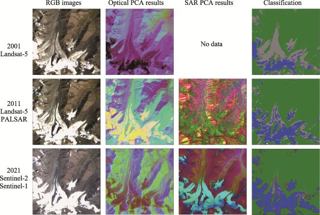
Figure 3 RGB composite maps of different source images (Column 1), PCA principal component analysis results of optical remote sensing data (Column 2), PCA principal component analysis results of SAR radar remote sensing data (Column 3), classification results after combining PCA major bands alone (2001) and two types of PCA major bands from 2011 and 2021 (Column 4), no available SAR radar remote sensing data in 2001
Several pixel-based machine learning methods are available on GEE, and RF, SVM, GTB, and CART were applied to classify the satellite images, each method had been debugged with different parameters and the best performing parameter settings had been applied, then the recognition accuracy of each method was compared. To evaluate the performance of the classification algorithm and the model accuracy, different accuracy measures were considered: the overall accuracy (OA) was the ratio of the total number of correctly classified pixels to the total number of pixels, and the kappa coefficient was used to indicate the degree of agreement between ground truth data and predicted values. After testing, RF led to the highest classification accuracy (Figures 4 and 5), so it was used to identify and classify the glaciers in the whole region. The RF classifier consists of a set of decision trees, where each tree is constructed by randomly selecting bootstrap samples from the original dataset. Each tree consists of multiple nodes, and a subset of randomly selected features, such as spectral information, is created at each node. The final classification of an object depends on the majority result of all trees (Breiman, 2001). The RF model requires the determination of two key initialization parameters, the number of classification trees or bootstrap iterations (Ntree) and the number of categorical features referenced in each classification (Mtry). For Ntree, the classification effect of the random forest classifier was computed from 10 to 500 in steps of 10 and found that the classification accuracy was high without affecting the computational performance when Ntree set to 200. For Mtry, the arithmetic square root of the total number of features in the training sample was used, and the value was set to 2. The study area was divided into 0.5° × 0.5° geographic grid cells to run the classifier to ensure the original pixel accuracy.
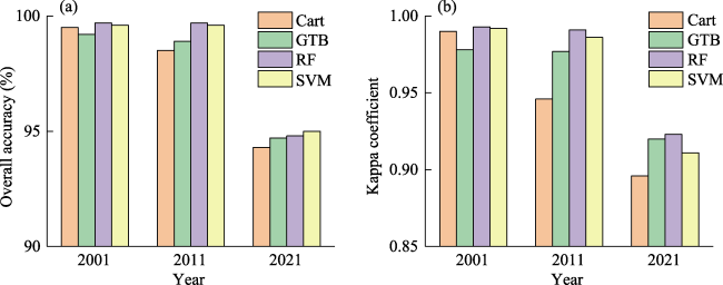
Figure 4 Overall accuracy (a) and kappa coefficient (b) of four machine learning methods, classification and regression tree (CART), gradient tree boost (GTB), random forest (RF), and support vector machine (SVM), in three different time periods for Dzhungarsky Alatau
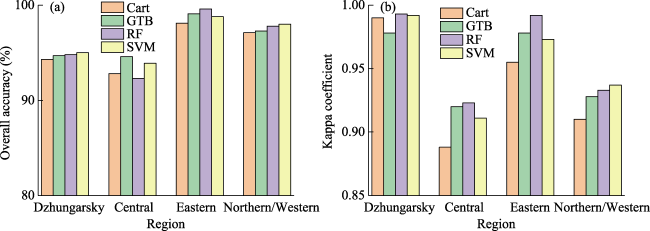
Figure 5 Overall accuracy (a) and kappa coefficient (b) of four machine learning methods in four different regions of the Tianshan Mountains in 2021
In pixel-based remote sensing image classification, the ‘salt and pepper’ effect is a familiar noise problem that occurs when the same features (neighbouring pixels) on an image are classified into different categories. Two methods were used to eliminate the salt and pepper classification error. One approach applied a spatial filter based on GEE’s ‘connectedPixelCount’ function, which identifies groups of pixels with the same pixel values based on their adjacency. Only pixels that did not meet a predefined connectivity criterion (i.e., the minimum number of connected pixels with the same value) were defined as isolated pixels and were reclassified, and the minimum number of grouped pixels for glaciers was set to 5. Additionally, a GEE-based segmentation clustering algorithm was applied, in which various seedGrid sizes were examined. A seedGrid size of 5 was selected due to its superior noise reduction capabilities and manageable computational power requirements. Following segmentation of classification results by seedGrid, images were clustered using the Simple Non-Iterative Clustering (SNIC) algorithm to minimize noise. After comparison, the ‘connectedPixelCount’ function was chose to eliminate the ‘salt and pepper’ effect, lastly, a threshold of 0.01 km2 was imposed to eliminate voids within the classification outcomes. After eliminating as much ‘salt and pepper’ noise as possible by using GEE-based segmentation clustering algorithm, the accuracy of the machine learning classification of glaciers was evaluated on GEE using the validation dataset.

3.2.2 Extracting glacier boundary and area

After obtaining the annual glacier identification classification results, the classified images were cropped to obtain the annual glacier raster using the glacier contours in the RGI. Considering that the RGI is more often drawn with images around 2010 in the study area, the 100-m buffer generated by the RGI6.0 contours was used to obtain the 2001 glacier extent based on visual inspection. Some of the glaciers missed by RGI6.0 were supplemented using RGI2.0. The cropped glacier raster was vectorized locally to extract the glacier profiles, and the DEM and RGI glacier profiles were used to generate component ice ridges to segment the glaciers. Finally, glacier parameters such as glacier area, mean aspect, and mean slope were calculated.

3.2.3 Evaluation of classification accuracy

Two aspects need to be considered to assess the accuracy of classification results: the classification accuracy of machine learning and the uncertainty of glacier area calculation. As mentioned earlier, random sampling was used to generate a training dataset for machine learning classification for 70% of each category in the dataset and a validation dataset for model accuracy evaluation for the remaining 30%. The accuracy of the classification was determined using the overall accuracy and kappa coefficient.
The buffer method was used to estimate the uncertainty in the glacier area calculation, which assumed that the maximum error in area determination was within the range of half a pixel and estimated this error by generating a buffer of half a pixel of the glacier boundary, using 15 m (half size of Landsat 5 and 7 pixels) as the buffer size for the classification results in 2001 and 2011. For the 2021 glacier identification boundaries, 5 m (half size of Sentinel-1 and Sentinel-2 pixels) was used as the buffer value. Statistically, the uncertainty of the glacier area calculation was determined to be ~2.6%, ~2.5%, and ~1.8% for 2001, 2011, and 2021, respectively.

4 Results

4.1 Accuracy assessment

As previously described, 30% of the 15,000 sample points for each year were randomly selected as the validation dataset to evaluate the accuracy of the RF model. After noise removal, the OA in 2001, 2011, and 2021 were improved compared to those before filtering, with values of 93.6%-99.7%, 96.0%-99.6%, and 94.7%-99.4%, respectively, and the kappa coefficients ranged from 0.889-0.996, 0.932-0.987, and 0.903-0.987 (Figure 6). Among the sub-regions, the lowest overall accuracies were found in the Central Tianshan, with values of only 93.6%, 96.0%, and 94.7%, respectively, and the kappa coefficients were 0.889, 0.938 and 0.912. In contrast, the Eastern Tianshan had the highest overall accuracy and the highest kappa coefficients. Among the local feature classifications, the overall accuracy of ice and snow identification was the highest, at almost 100%, although there was some confusion between ice and snow. Debris were identified with the lowest accuracy, and although some debris were identified accurately, there were cases where they were identified as ice or other features; however, overall, debris could be better distinguished from other features (Table 2).
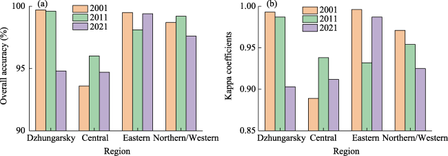
Figure 6 Overall accuracy (a) and kappa coefficient (b) of RF in four different regions of the Tianshan Mountains in 2001, 2011, and 2021
Table 2 Example of confusion matrix for different feature classifications, with data from the 2011 Central Tianshan Mountains classification results
Ice Snow Debris Others
Ice 5127 124 0 2
Snow 195 1532 1 1
Debris 1 1 1963 206
Others 0 4 194 8990
Based on the vectorized glacier profile, the uncertainty of glacier area was obtained by buffering, and we calculated the statistical error of glacier area from 2001 to 2021 for the three periods as ±353.87 km2, ±310.80 km2, and ±200.90 km2. Specifically, 2021 had a finer pixel resolution (10 m), and therefore, the error was minor compared to that in 2001 and 2011 (pixel resolution of 30 m).

4.2 Spatial and temporal changes in glacier area

The glacier areas in 2001, 2011, and 2021 for the four sub-regions (Central Tianshan, Dzhungarsky Alatau, Eastern Tianshan, and Northern/Western Tianshan) of the Tianshan were calculated on GEE using multisource remote sensing data and analysed their changes (Figure 7). The largest regional glacier area was in Central Tianshan, which accounted for 60% of the total glacier area in the Tianshan. The glacier area of Dzhungarsky Alatau was relatively small, only approximately 7% of the size of the glacier area in the Central Tianshan. The average area of a single glacier in the Central Tianshan was also larger than that in other regions. Across the Tianshan, glacier area decreased from 13,610.33 ± 353.87 km2 to 12,431.83 ± 310.80 km2 from 2001 to 2011, a loss of 1178.50 km2 at a rate of 0.87%/a, while glacier area decreased to 10,573.93 ± 200.90 km2 from 2011, which was a rate of 1.49%/a, showing an accelerated retreat overall compared to the previous decade.
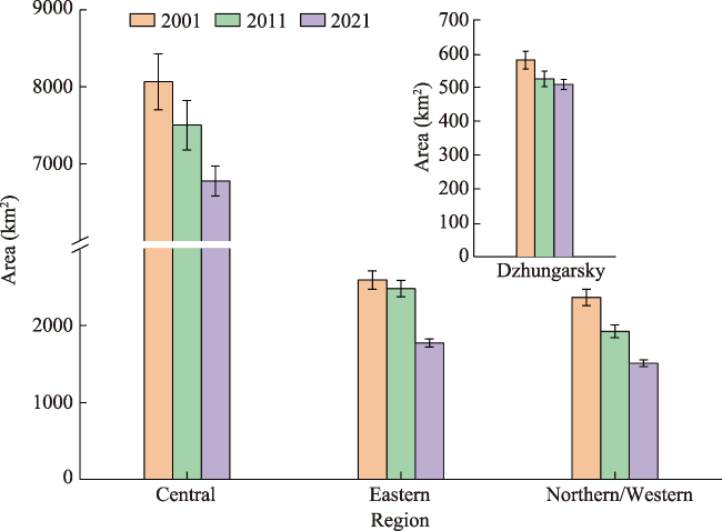
Figure 7 Glacial areas in the four sub-regions of the Tianshan Mountains in 2001, 2011 and 2021, with error bars indicating the error of the area counted from the buffer zone
Although glacier area has decreased in all sub-regions since 2001, they have had different trend patterns. The decrease in glacier area in Dzhungarsky Alatau from 2011 to 2021 was significantly lower than that from 2001 to 2011, i.e., a ‘slower retreat.’ Although glacier area retreat has accelerated in the other three sub-regions in the last decade, the inter-annual rate of change in the central and Northern/Western Tianshan was more stable and increased less, while the rate of glacier retreat in the Eastern Tianshan increased significantly in 2011-2021 compared to the previous decade. Specifically, the glacier areas in Dzhungarsky Alatau, Central Tianshan, Northern/Western Tianshan, and Eastern Tianshan decreased by 57.29 km2, 566.44 km2, 442.44 km2, and 112.32 km2 during 2001-2011, at rates of 0.98%/a, 0.70%/a, 1.86%/a, and 0.43%/a, respectively, while the loss rates for 2011-2021 were 0.27%/a, 0.96%/a, 2.14%/a, and 2.84%/a, indicating glacier area reductions of 14.28 km2, 724.24 km2, 412.54 km2, and 706.83 km2, respectively. It is important to note in particular that the Northern/Western Tianshan has consistently exhibited a high rate of retreat since 2001, with a value of almost 2.00%/a (Table 3).
Table 3 Glacial area changes (GAC) and corresponding average annual area change rates (ACR) from 2001 to 2011, 2011 to 2021 and 2001 to 2021 in four sub-regions of the Tianshan Mountains
Sub-regions GAC (km²) 2001-2011 GAC (km²) 2011-2021 GAC (km²) 2001-2021 ACR (%/a) 2001-2011 ACR (%/a) 2011-2021 ACR (%/a) 2001-2021
Dzhungarsky Alatau -57.29 -14.28 -71.56 -0.98 -0.27 -0.61
Central Tianshan -566.44 -724.24 -1290.68 -0.70 -0.96 -0.80
Eastern Tianshan -112.32 -706.83 -819.15 -0.43 -2.84 -1.58
Northern/Western Tianshan -442.44 -412.54 -854.99 -1.86 -2.14 -1.81
The evolution of glacier areas within each sub-region also showed significant differences. The Tianshan was divided into 0.5°×0.5° geographic grid cells and analysed the trend of glacier area change in different grid cells (Figure 8). Overall, the majority of glacier areas within the geographic grid cells show shrinkage at diverse rates of magnitude. Glacial retreat was more severe in mountain peripheries, river valleys, and gentler areas than in higher elevation mountains. The areas with the most dramatic changes in area values were located at the junction of the western part of the Central Tianshan with the eastern part of the Northern/Western Tianshan, the western part of Eastern Tianshan and the western part of Northern/Western Tianshan. Although the values of area reduction were substantial, the relative rates of change were not necessarily more significant than those in other regions, particularly in the Central Tianshan (approximately 80°E). Specifically, in the Tomur-Khan Tengri region, a positive glacier area growth of 0.2%/a-0.4%/a was observed between 2001 and 2011, while a shrinkage rate of -0.02 to -0.4%/a between 2011 and 2021, indicating an anomalous steady state. The glacier area loss in the interior of the Dzhungarsky Alatau exceeded that in its surrounding areas, yet the rate of area retreat in the surrounding areas surpassed that in the interior. A region of significant positive glacier area growth is present in the Eastern Tianshan near 88°E, and the rate of retreat in other regions has accelerated over the past decade. This acceleration in the rate of retreat is also widespread in various geographic grid cells of the northwestern Tianshan, exhibiting a more extensive distribution.
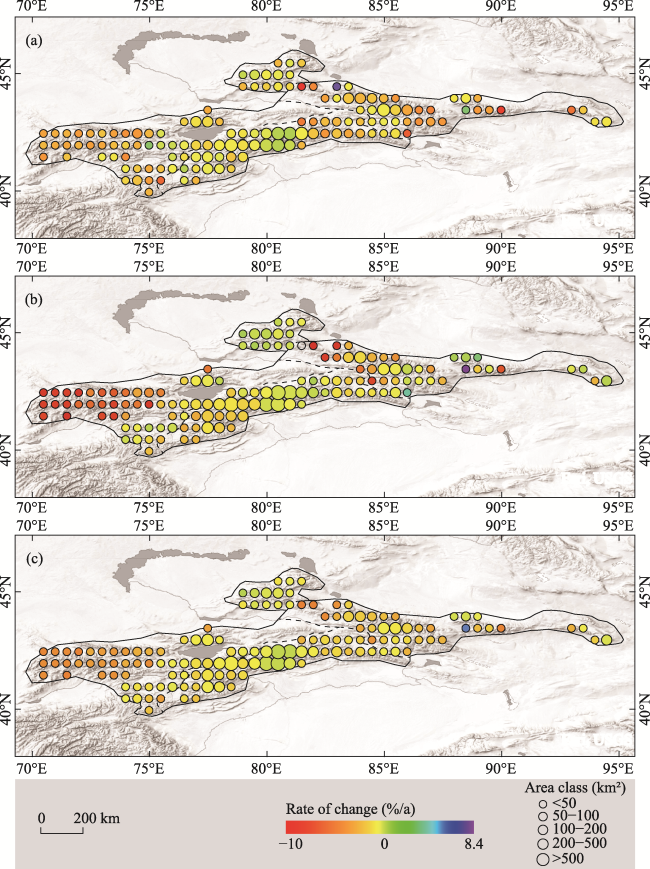
Figure 8 Annual mean area change rates of 2001-2011 (a), 2011-2021 (b) and 2001-2021 (c) for the different sub-regions of the Tianshan Mountains (using 0.5° grid cells derived from HiMAP). Pie sizes represent the glacier area in each sub-region. Purple boundaries indicate the four mountain sub-region boundaries of the Tianshan in HiMAP.

4.3 Variation in glacier area with different topographic factors

The glaciers in the Tianshan are distributed at 2200-7500 m a.s.l., with more than 95% of the glacier area mainly distributed at 3400-5400 m a.s.l., i.e., near the glacier equilibrium line. Dzhungarsky Alatau is at a lower altitude, so its glacier distribution altitude band is also lower than those of the other three regions, and its glacier terminus can reach a minimum altitude of approximately 2200 m a.s.l. (Figure 9).
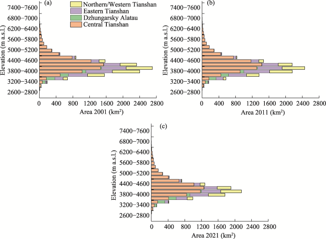
Figure 9 Area-altitude distribution of the four sub-regions of the Tianshan Mountains in 2001 (a), 2011 (b), and 2021 (c)
However, the glaciers distributed at approximately 2200-2400 m a.s.l. in 2001 completely disappeared after 2011. The Central Tianshan has the highest average elevation and, therefore, the most elevation bands spanned by glacier distribution in its region. The glacier equilibrium line in Dzhungarsky Alatau was much lower than that in the Central Tianshan. Our results show that, in terms of altitudinal band distribution, the most drastic reduction in glacier area has been in the range of 3400-3600 m a.s.l., with 671.38 km2, 569.21 km2, and 417.99 km2 of glacier area in the three phases, respectively, and a loss of 253.39 km2 at a rate of 1.89%/a. The four sub-regions with the most severe loss of glacier area were 3800-4000 m a.s.l. in the Central Tianshan, 3000-3200 m a.s.l. in the Eastern Tianshan, 3200-3400 m a.s.l. in the Northern/Western Tianshan, and 3000-3200 m a.s.l. in Dzhungarsky Alatau. Part of the glacier elevation was more significant than 5800 m a.s.l. Changes occurred relatively steadily, where the loss was slight, and the shrinkage rate was only 0.3%/a or less, and the proportion of glacier area to the total area in this region even slightly increased. Only approximately 1.6%-1.7% of the glacier area was distributed at elevations below 3400 m a.s.l.
The median elevation is commonly used to estimate the equilibrium line height, so it describes the height position in glacier topographic analysis. Our results showed that the median elevation of glaciers of different area classes was above 4000 m a.s.l., and it is increased with the glacier area. Among the different glacier size categories, glaciers in the smallest area class (0-1 km2) had a more significant median elevation distribution but a narrower elevation range, while glaciers in the larger area class had a more comprehensive elevation range but a closer median elevation distribution (Figure 10a).
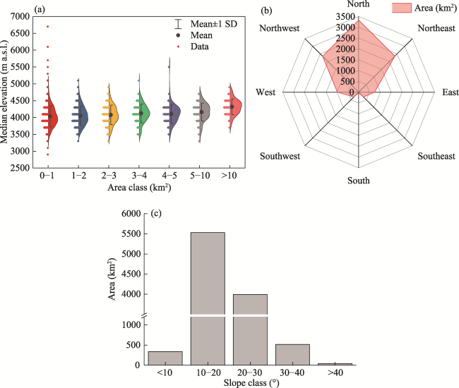
Figure 10 Distribution of the median elevation of glaciers by size class (the violin plot) and the number of glaciers in each class (the bar plot) (a); The distribution of glacier area by mean aspect (summed to eight directions) (b); Histogram of glacier area represented by average slope (c)
In terms of slope distribution, northwest, north, and northeast were the main directions of glacier distribution in the Tianshan, where the area of glaciers with north as the main direction accounted for approximately one-third of the glacier area, while those with the northwest and northeast directions accounted for 17.6% and 15.7% of the area, respectively (Figure 10b). It should be noted that in the area of the prominent peak of the Tianshan, the main directions of some massive valley glaciers, such as the Tomur Glacier, the North-South Inilchek Glacier, and the Tugai Berezi Glacier, were southwest, west, and east, respectively. However, most of the glaciers at the edge of the mountain range have developed towards the north, and most of the glaciers with more area loss are also in this direction. The average slope of glaciers in the Tianshan is 25°, and the larger the glacier area is, the gentler its average slope is. In terms of slope gradation, more than 5500 km2 of glaciers have an average slope between 10° and 20°, accounting for approximately 40% of the glaciers, and more than 5000 km2 of glaciers have an average slope gradient between 20° and 30° (Figure 10c). A tiny percentage of glaciers have average slopes less than 10° and greater than 40°, and the remaining < 1000 km2 of glaciers have average slopes steeper than 30°. A significant reduction in glacier area occurred in the less than 10° and greater than 40° slope bands (Figure 10c).

5 Discussion

5.1 Uncertainty analysis

Discussing the causes of uncertainty generation is essential to improve the accuracy of glacier identification and accurately verify the glacier area variation. The uncertainty in our results had two main components: the classification error when the machine learning algorithm was run on GEE and the error generated when the glacier profile was depicted.

5.1.1 Uncertainty of glacier classification

GEE effectively improves the speed of parallel processing of massive image data (Gorelick et al., 2017). However, the pixel-based classification of annual composite images using machine learning algorithms on GEE is also subject to limitations such as memory usage and data size of GEE itself, the type of machine learning algorithms and the setting of algorithm parameters, the time and feature differences of the images selected for annual image synthesis, the selection of training data and validation data and their authenticity, the choice of band combinations and indices, and the degree of classification noise elimination.
As described in the methodology, the current work was analysed by dividing the large area into 0.5°×0.5° grids, running the algorithm separately and then merging the results to avoid generating mixed image elements to affect the classification accuracy (Xie et al., 2020). Although the RF calculation is time-consuming and self-fitting or overfitting occurs when the number of set trees is large, it has the highest classification accuracy; therefore, RF was chosen as the applied classification algorithm and set the number of input trees to 200, whose final overall accuracy was high and acceptable.
The image which input to the algorithm resulted from a median composite of multiple declouded images. It has been suggested that mapping glaciers in a single image may be more advantageous than mapping them in an annual composite image because the composite image may be affected by seasonal and annual differences (Bevington and Menounos, 2022). Some clouds and smoke may be merged into the composite image to produce subtle errors that are not easily detected (Qu et al., 2021). It has also been shown that the median composite image has the highest classification accuracy (Qu et al., 2021). Image selection was restricted to May through October to avoid the effects of seasonal snow. However, some alpine areas may still have snow, which can obscure the determination of glacier boundaries, and some seasonal snow can produce significant errors in glacier size estimates for smaller areas. Therefore, images with low or no clouds were selected as much as possible, but clouds are inevitable at certain times or in certain places. Even after strict cloud mask filtering (Sentinel-2) or manual filtering (high reflectivity parts of the Landsat series images such as ice and snow are quickly treated as clouds in the cloud mask (Zhu et al., 2018), some thin clouds or shadows can still affect the performance of the algorithm, and the actual value of some image elements may be affected.
The training and validation datasets were selected based on expert knowledge and manually delineated on annual synthetic images with the assistance of high-resolution images from Google Earth. At the boundary of glaciers, due to the limitation of the pixel spatial resolution and the small size of some glaciers, there were a number of mixed pixels consisting of glaciers and other features. These mixed pixels are one source of error in pixel-based supervised classification, and their types are delineated based on expert experience, which also increases the uncertainty of glacier classification.
Some mature spectral indices or band ratios were added to the raw bands and performed principal component analysis, including factors such as the NDSI, NDVI, and BSI, which help to distinguish some feature categories with similar spectral reflections, such as supra-ice ponds or flow (Shukla, Gupta, and Arora 2009; Tedesche et al., 2019). The addition of SAR data can effectively distinguish special feature categories, such as surface debris with an undulating surface that is not affected by clouds, and the elevation and slope can help to select ice and snow samples more accurately (Lu et al., 2020). Combining SAR data with the optical sensor can help to improve the accuracy of the classification results (Figure 11), and this approach is more accurate than the single output of each (Table 4).
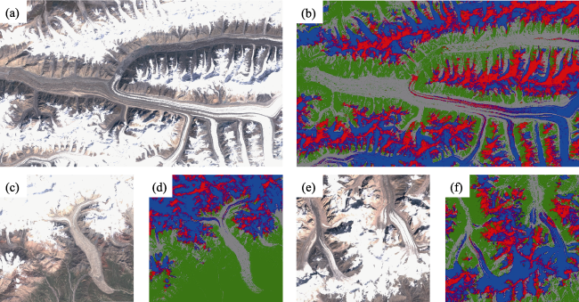
Figure 11 Some examples of classification of debris-covered glaciers. (a), (c), and (e) are Sentinel-2 RGB composites, (b), (d), and (f) are classification results, green represents other features including water, gray represents debris, blue represents clean ice, and red represents snow.
Table 4 Overall accuracy and kappa coefficients of different PCA components in the Eastern Tianshan Mountains in 2021. S1_PCA represents the PCA results generated by Sentinel-1, S2_PCA represents the PCA results generated by Sentinel-2, S1S2_PCA represents the PCA bands after synthesis of PCA results generated by Sentinel-1 and Sentinel-2.
Parameters S1_PCA S2_PCA S1S2_PCA
Overall accuracy (%) 70.92 91.24 99.55
Kappa coefficient 0.34 0.84 0.94
Salt and pepper noise is unavoidable for supervised pixel-based classification incorporating SAR data, especially in some parts of surface debris, bare ice, ice, and water that produce mixed image elements. This noise affects the accuracy of the classification, and as described in the methods section, this noise has eliminated as much as possible. The different numbers of convolution kernels and maximum connected pixels have different effects on noise removal. It was determined experimentally that a 5×5 kernels with 50 connected pixels was appropriate to avoid eliminating the correctly classified pixels, though there may be better parameter settings for this approach (Xie et al., 2020). Several studies have also indicated that object-based classification methods may be more effective in removing noise to improve accuracy (Boonprong et al., 2018), but comparing their effectiveness with pixel-based classification is still needed. In 2021, due to the higher resolution of Sentinel-1 and Sentinel-2 than the Landsat series and PALSAR/PALSAR-2, some features that behaved as mixed pixels in the Landsat series and PALSAR/PALSAR-2 were more clearly distinguished in 2021, but more noise was generated as a result, especially in the SAR images acquired from Sentinel-1. This resulted in lower classification accuracy based on SAR images in 2021 and reduced the overall accuracy, but this reduction in overall accuracy was acceptable compared to the more accurate distinction of different kinds of feature.

5.1.2 Uncertainty in the statistical analysis of glacier area

A raster-to-polygon local operation was performed on the postprocessed classification results and generated buffers to estimate the uncertainty in the glacier area statistics using half a pixel resolution as the buffer threshold. The buffers were 15 m for the Landsat series data and 5 m for the Sentinel series data. The statistical errors of glacier area from 2001 to 2021 for the three periods were ±353.87 km2, ±310.80 km2, and ±200.90 km2, so the uncertainties in 2001 and 2011 were slightly more considerable than those in 2021, with values of 2.6%, 2.5% and 1.9%, respectively. The classification raster was clipped based on the RGI, and due to the buffer setting mentioned in the method, some snow or extra glacial debris from alpine areas or the end of a glacier may have been included in the glacier extent. Some areas of the original glacier inventory were missing, and although we tried to fill in the missing glacier as much as possible, there may be some smaller glaciers that have not been added. Due to the presence of noise and the mask created by some water bodies on ice, some data holes were inevitably created in the identified glaciers, and the holes smaller than 0.01 km2 were eliminated based on the RGI and expert experience. The accuracy of the final results was similar to the results of the glacier inventory and other studies (Lea 2018; Smith et al., 2020), indicating that the results are reliable.
It is necessary to discuss the applicability of different resolution classification results for direct comparison in this study, and the classification raster in 2021 was resampled from 10 m resolution to 30 m resolution and the area and its error were counted. The area of glacier extraction in 2021 after resampling was 9865.38 ± 236.90 km2, which is smaller than the area before resampling, and the percentage of glacier area in the four sub-regions was basically the same as before resampling. The results of the analysis using the resampled glacier area were not significantly different in terms of important conclusions such as the accelerated retreat trend in Eastern Tianshan and the slower retreat in Dzhungarsky Alatau, except that the glacier retreat is more severe, which indicated that it is feasible to directly use the 10m resolution classification results before resampling for the analysis, and the resolution advantage of the Sentinel series images can be exploited.

5.2 Comparison with other regions across the Tianshan

Some studies have similarly reported that the most intense glacier retreat in the Tianshan is generally distributed in the outer mountain ranges and lower elevations near densely populated plains or river valleys, e.g., Narama et al., (2010) examined four regions and found that the most significant changes occurred in the periphery, with a 19% change (~0.63%/a) between 1970 and 2000. Bolch (2007) used Soviet glacier inventories and Landsat data to examine the Zariiski and Kungui Alato valleys in the northern Tianshan and found a >32% decrease (~0.72%/a) between 1955 and 1999, while in the more immense glaciers and higher elevation interior alpine areas, studies found that they have shown relative stability in recent years (Milner et al., 2017). These results corroborate the validity and accuracy of our work. In terms of sub-region scale, it was found that glaciers in the Eastern Tianshan and Dzhungarsky Alatau have most significant negative mass balance rate (Barandun et al., 2021). In contrast, the annual mass balance variability was lower in the Central Tianshan (Barandun et al., 2021), and the glacier area shrinkage rate in the Northern/Western Tianshan had spatial variability ranging from 0.11%/a to 3.7%/a (Zhang et al., 2021), which was more consistent with our results. Huang et al. (2021) suggested that the glacier area shrinkage rate in the Eastern Tianshan was 0.8%/a between 1990 and 2018, but our results show that the glacier loss rate in the Eastern Tianshan consistently exceeded 2%/a. Our results indicate a stable and minimal increase in glacier area in this region between 2001 and 2011, followed by a subtle decreasing trend between 2011 and 2021, which aligns with the findings of other researchers. Zhou et al. (2021) found that this region encompasses nearly all the surge glaciers and advancing glaciers in the Tianshan, with advances ranging from several hundred meters. These glaciers are larger in size, and their advancing portions contribute more significantly to glacier area change compared to smaller glaciers. Li et al. (2018) similarly concluded that the glacier mass balance in this region from 2000 to 2011 was much lower than in other regions of the Tianshan. Table 5 offers comparisons of our results in various regions with the glacier area shrinkage rate from previous studies. An accelerating trend of glacier retreat has been observed in recent years (Wan et al., 2020), while earlier studies have reported less glacier change in the past decade. Based on this comparison, the glacier area shrinkage rate derived from our study for the first and second decades of the 21st century is consistent with those found in other studies. For some smaller glaciers or those located at the periphery of mountain systems, they are more sensitive to climate change. Although their absolute area change values may not be larger than those of larger glaciers, their relative glacier area change rates will be more pronounced. The above comparisons show that our work on identifying and classifying glaciers at large regional scales with high spatial resolution on the GEE is reliable. Such a process is helpful for annual glacier mapping to obtain a quick and accurate picture of their changes.
Table 5 The average glacier area change rate in this study compared with the previous studies
Region Time ranges Average area change
rates (%/a)
References
Eastern Tianshan near Hami 1960s-2010 -0.66 Che et al. (2018)
2001-2011 -1.47 This study
Eastern Tianshan near Turpan 1960s-2010 −0.86 Che et al. (2018)
2001-2011 -1.98 This study
Dzhungarsky Alatau and the western part of the Eastern Tianshan 1960s-2010 -0.72 Che et al. (2018)
2001-2011 -1.78 This study
Eastern Tianshan near Hami CGI-1 and CGI-2 -1.36 - -1.66 Su et al. (2022)
2001-2011 -1.47 This study
Eastern part of the Central
Tianshan
2012-2014 -2.82 Liu et al. (2020)
2011-2021 -2.17 This study
Eastern Tianshan 2000-2020 -2.98 Zhang et al. (2021)
2001-2021 -1.56 This study
Part of the Central Tianshan 2000-2010 -0.73 Zhang et al. (2021)
2001-2011 -0.70 This study
2000-2020 -1.07 Zhang et al. (2021)
2001-2021 -0.80 This study
Headwater region of the Urumqi River 2001-2011 -2.59 Zheng et al. (2022)
2001-2011 -2.53 This study
2011-2017 -3.01 Zheng et al. (2022)
2011-2021 -3.03 This study
Dzhungarsky Alatau and the western part of the Eastern Tianshan 2000-2015 -0.68 Zhang et al. (2022)
2011-2021 -0.71 This study
Aksu River Basin 1975-2016 -0.63 Zhang et al. (2019b)
2001-2011 -0.66 This study
2011-2021 -0.88
Tuyuksu Group of Glaciers 1998-2016 -0.53 Kapitsa et al. (2020)
2001-2011 -1.76 This study
2011-2021 -1.42

5.3 Glacial response to climate change and topographic factors

2 m temperature and total precipitation from ERA5-Land Monthly Averaged by Hour of Day reanalysis data were chosen to analyse the distance-level changes in summer and winter mean temperature and precipitation in the Tianshan for 2001-2011 and 2011-2021 compared to the previous decade (Figure 12), where June-August were defined as summer and December-February were defined as winter. The temperature changes in the Tianshan since 2001 showed inconsistent spatial variability. Summer temperatures showed varying degrees of upwards trends, while winter temperatures showed only weak negative pitch levels from 2001 to 2011 in parts of Dzhungarsky Alatau and the Eastern Tianshan, but from 2011 to 2021, the negative pitch levels increased significantly, particularly in mountainous regions. The variation in summer precipitation exhibited considerable spatial variability. High mountainous areas of the Central Tianshan and its adjacent regions, including the Northern/ Western Tianshan and Eastern Tianshan, as well as the mountainous regions of the Dzhungarsky Alatau, demonstrated an increase in precipitation between 2001 and 2011. Meanwhile, the remaining areas displayed various degrees of precipitation decline. Precipitation in the Northern/Western Tianshan continued to exhibit a negative pitch level during the summer of 2011-2021. However, most of the mountainous regions of the Eastern Tianshan experienced increased precipitation during the same period. The trend of winter precipitation remains unclear, except for the Northern/Western Tianshan, where it transitioned from progressively wet to progressively dry. In general, summer precipitation increases slightly in mountainous areas and decreases gradually in the surrounding valleys and plains.
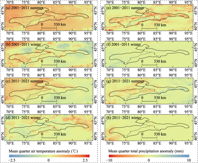
Figure 12 ERA 5-Land composite anomaly map by summer and winter (difference between epochs 2001-2011 and 2011-2021) for average total monthly precipitation anomaly (Column 1, a-d) and mean monthly air temperature anomaly (Column 2, e-h).
Summer temperatures mainly control glacier ablation and winter precipitation mainly regulates glacier accumulation (Bonekamp et al., 2019), and precipitation in the Tianshan region is mainly concentrated in summer (Guan et al., 2021a, 2021b). Although summer precipitation has increased, its relatively small proportion of precipitation has had a much smaller impact on glaciers than summer temperatures. The continued increase in summer temperatures can be considered an important driving force contributing to the continued shrinkage of glaciers in the Tianshan. Specifically, augmented summer precipitation and negligible alterations in summer temperature in the regions near 80°E in the Central Tianshan and 88°E in the Eastern Tianshan may provide a plausible explanation for the observed expansion of glacier areas in these regions.
Some topographic factors, such as elevation, slope, and slope direction, influence glacier variability (Liu et al., 2013). It has been confirmed that increases in temperature and precipitation lead to differences in elevation-related snow cover area expression (Kunkel et al., 2016), with a decrease in snow cover area at lower elevations and an increase at higher elevations, similar to the decrease in glacier area at lower elevations and the stabilization in glacier area at higher elevations shown in our results. Glaciers in the Tianshan are primarily located in the lower elevation zone (3600-4600 m a.s.l.), a region with higher temperatures and less precipitation than those observed in higher elevations, where glaciers continue to retreat, a result that is close to the results provided by Shangguan et al., (2009), who found that the most significant reductions in the glacier area occurred at elevations of 4100-4500 m a.s.l. Our results found that glaciers in smaller area classes (0-5 km2) had much larger relative area loss rates, although they were smaller than those in larger area classes (5-10 km2 and >10 km2). Many small glaciers have small accumulation areas, receive limited accumulation and are more sensitive to the temperature rise, so their retreat is more severe. The convergence of several branch glaciers forms some large composite valley glaciers, and their accumulation areas are higher in elevation and widely distributed. Some accumulation areas are gentler than small glaciers, and the higher elevation areas are thinner but stable in area change when precipitation increases in higher mountain areas. However, the terminal elevations of these large valley glaciers are usually lower, and thus their glacier terminals are subject to significant ablation by increasing temperatures. The orientation of the glacier is closely related to the intensity of surface solar radiation it receives, so the average slope orientation determines the accumulation and melting rates of the glacier to some extent (Olson and Rupper 2019). The surface solar radiation received on the south side of the mountain range is much higher than that on the south side of the mountain range, and thus, more glaciers are developed on the north side of the mountain range than on the south side (i.e., glaciers with N, NW, and NE as the average slope orientation are more predominant). In addition, glaciers on the south side of the watershed in some areas have declined more than those on the north side, reflecting the difference in solar radiation received by the north and south sides of glaciers. The mean slope of glaciers varies significantly from region to region. It is mainly related to the mean slope of the catchment, with some larger glaciers having a more comprehensive altitudinal range and, therefore, a more significant mean slope; moreover, smaller overhanging glaciers may have a more significant mean slope and may be distributed over a wide range of altitudes. Some studies have also indicated that the debris coverage of some glaciers in Central Asia has increased as the glaciers continue to shrink (Scherler et al., 2011; Kääb et al., 2012; Milner et al., 2017). Debris, which usually covers the end of the ice tongue and may be continuous from higher elevations to the glacier below, also has a significant influence on the glacier ablation. Thin debris accelerates glacier melting by reducing the albedo of the glacier surface, but debris thicker than a few centimetres may inhibit glacier ablation by isolating heat exchange between ice and air. Because the statistics of glacier area were not continuous in time, the effect of surface debris is not discussed further here, although it was clear from the area change that some surface debris-covered glaciers have retreated at a faster rate than glaciers not covered by surface debris.
The analysis of the causes of glacier changes in the Tianshan is similar to the conclusions of others in that changes in the degree of glacier retreat depend on climatic and topographic conditions to some extent (Sorg et al., 2012; Farinotti et al., 2015; Kraaijenbrink et al., 2017; Pritchard, 2019). Studies have shown that since the 1980s, the Central Asian region where the Tianshan is located has experienced a transition from warm-dry to warm-wet, i.e., an increasing trend in temperature and precipitation (Zhang et al., 2019a; Yao et al., 2021). The high mountain ranges of the Tianshan intercept the moisture carried by the air currents from the mid-latitude westerly wind belt to generate precipitation, and the convergence between the westerly wind belt disturbances and the atmospheric circulation from the Siberian high pressure has a triggering effect on the precipitation in the mountains (Yao et al., 2016). It has been suggested that the Scandinavia (SCAND) teleconnection pattern represents important circulation variability affecting Tianshan summer precipitation, and the vigorous high pressure over the Ural Mountains and the low pressure over Central Asia during the SCAND negative phase in summer jointly lead to enhanced moisture transport from the Arctic Ocean to the Tianshan (Guan et al., 2021b). It has also been suggested that climate forcing is the primary driver of sensitivity to uneven changes in material balance in alpine Asia, explaining up to 60% of the spatial variation in glacier variability (Sakai and Fujita 2017), while glacier morphology has been found to explain up to 36% of the spatial mass balance variability in the Tianshan (Brun et al., 2019).

6 Conclusions

Using Sentinel-1/2, Landsat 5/7/8, PALSAR/PALSAR-2, NASADEM and ALOSDSM, as well as ERA-5 land data, based on machine learning algorithms on the Google Earth Engine platform, the maps of glacier distribution in the Tianshan of 2001, 2011, and 2021 were generated.
Using the main components obtained from PCA processing of SAR images and optical images for inputs of machine learning algorithms based on the GEE platform can improve the overall identification accuracy. Compared with support vector machine, gradient tree boost, and classification and regression tree, random forest was the classifier with the highest kappa coefficients in this paper’s approach, reaching 0.916-0.994 in identifying ice, and the overall accuracy reached over 90%. The uncertainty of the glacier area calculation was determined to be ~2.6%, ~2.5%, and ~1.8% for 2001, 2011, and 2021, respectively.
Glaciers in most regions of the Tianshan are in a state of accelerated retreat, with total glacier areas of 13,610.33 ± 353.87 km2, 12,431.83 ± 310.80 km2, and 10,573.93 ± 200.90 km2 in 2001, 2011, and 2021, respectively, and an overall rate of retreat accelerating from 0.87%/a in the previous decade to 1.49%/a in the latter decade. The trends were not consistent across sub-regions; the Eastern Tianshan glacier has retreated at the fastest rate, with a dramatic increase of more than five times in the last decade, and the rate of change in the Dzhungarsky Alatau in the last decade has decreased to one-third of that of earlier periods.
The most dramatic glacier retreat has been distributed near the glacier equilibrium line. Glacial retreat is more severe in the periphery of the mountains, lower plains, and valleys than in higher elevation regions. The increase in temperature and precipitation has caused some degrees of glacial changes in the Tianshan, with accelerated ablation of glacier ends and increased snow cover at higher elevations.
The method of identifying and classifying glaciers at large regional scales with high spatial resolution on the GEE in this paper is reliable, and this workflow facilitates the annual glacier mapping of regions of interest to obtain a quick and accurate picture of their changes. Water is classified under other features, and the selection of samples relies on the manual experience of experts and does not involve changes in the distribution of features within years. For future studies, random sampling of the sample set for different times can be attempted, and statistics are performed on each validation sample set to obtain a more accurate model performance. We expect to achieve more accurate and diverse classification of glacier features in the future by combining different times of the year and topography, and will explore the use of more advanced algorithms, such as deep learning, to improve the accuracy of automatic glacier identification.

Declaration of interest statement

The authors declare no potential conflict of interest.
[1]
Barandun M, Pohl E, Naegeli K et al., 2021. Hot spots of glacier mass balance variability in Central Asia. Geophysical Research Letters, 48(11): e2020GL092084.

[2]
Bevington A R, Menounos B, 2022. Accelerated change in the glaciated environments of western Canada revealed through trend analysis of optical satellite imagery. Remote Sensing of Environment, 270: 112862.

DOI

[3]
Bhattacharya A, Bolch T, Mukherjee K et al., 2021. High Mountain Asian glacier response to climate revealed by multi-temporal satellite observations since the 1960s. Nature Communications, 12(1): 1-13.

DOI

[4]
Bolch T, 2007. Climate change and glacier retreat in northern Tien Shan (Kazakhstan/Kyrgyzstan) using remote sensing data. Global and Planetary Change, 56(1/2): 1-12.

DOI

[5]
Bonekamp P N, De Kok R J, Collier E et al., 2019. Contrasting meteorological drivers of the glacier mass balance between the Karakoram and central Himalaya. Frontiers in Earth Science, 7: 107.

DOI

[6]
Boonprong S, Cao C, Chen W et al., 2018. The classification of noise-afflicted remotely sensed data using three machine-learning techniques: effect of different levels and types of noise on accuracy. ISPRS International Journal of Geo-Information, 7(7): 274.

DOI

[7]
Breiman L, 2001. Random forests. Machine Learning, 45(1): 5-32.

DOI

[8]
Brun F, Wagnon P, Berthier E et al., 2019. Heterogeneous influence of glacier morphology on the mass balance variability in High Mountain Asia. Journal of Geophysical Research: Earth Surface, 124(6): 1331-1345.

[9]
Cai X, Li Z, Zhang H et al., 2021. Vulnerability of glacier change in the Tianshan Mountains region of China. Journal of Geographical Sciences, 31(10): 1469-1489.

DOI

[10]
Che Y, Zhang M, Li Z et al., 2018. Quantitative evaluation of glacier change and its response to climate change in the Chinese Tien Shan. Cold Regions Science and Technology, 153: 144-155.

DOI

[11]
Chen Y, Li W, Deng H et al., 2016. Changes in Central Asia’s water tower: Past, present and future. Scientific Reports, 6(1): 1-12.

DOI

[12]
Deng H, Chen Y, 2017. Influences of recent climate change and human activities on water storage variations in Central Asia. Journal of Hydrology, 544: 46-57.

DOI

[13]
Farinotti D, Longuevergne L, Moholdt G et al., 2015. Substantial glacier mass loss in the Tien Shan over the past 50 years. Nature Geoscience, 8(9): 716-722.

DOI

[14]
Gorelick N, Hancher M, Dixon M et al., 2017. Google Earth Engine: Planetary-scale geospatial analysis for everyone. Remote Sensing of Environment, 202: 18-27.

DOI

[15]
Guan X, Yao J, Schneider C, 2021a. Variability of the precipitation over the Tianshan Mountains, Central Asia. Part I: Linear and nonlinear trends of the annual and seasonal precipitation. International Journal of Climatology, 42(1): 118-138.

DOI

[16]
Guan X, Yao J, Schneider C, 2021b. Variability of the precipitation over the Tianshan Mountains, Central Asia. Part II: Multi-decadal precipitation trends and their association with atmospheric circulation in both the winter and summer seasons. International Journal of Climatology, 42(1): 139-156.

DOI

[17]
Hagg W, Mayer C, Lambrecht A et al., 2013. Glacier changes in the Big Naryn Basin, Central Tian Shan. Global and Planetary Change, 110: 40-50.

DOI

[18]
Huang L, Li Z, Tian B S et al., 2011. Classification and snow line detection for glacial areas using the polarimetric SAR image. Remote Sensing of Environment, 115(7): 1721-1732.

DOI

[19]
Huang W, Duan W, Chen Y, 2021. Rapidly declining surface and terrestrial water resources in Central Asia driven by socio-economic and climatic changes. Science of the Total Environment, 784: 147193.

DOI

[20]
Huss M, Hock R, 2018. Global-scale hydrological response to future glacier mass loss. Nature Climate Change, 8(2): 135-140.

DOI

[21]
Ji F, Wu Z, Huang J et al., 2014. Evolution of land surface air temperature trend. Nature Climate Change, 4(6): 462-466.

DOI

[22]
Kääb A, Berthier E, Nuth C et al., 2012. Contrasting patterns of early twenty-first-century glacier mass change in the Himalayas. Nature, 488(7412): 495-498.

DOI

[23]
Kapitsa V, Shahgedanova M, Severskiy I et al., 2020. Assessment of changes in mass balance of the Tuyuksu Group of Glaciers, Northern Tien Shan, between 1958 and 2016 using ground-based observations and Pléiades satellite imagery. Frontiers in Earth Science, 8: 259.

DOI

[24]
Kraaijenbrink P D A, Bierkens M F P, Lutz A F et al., 2017. Impact of a global temperature rise of 1.5 degrees celsius on Asia’s glaciers. Nature, 549(7671): 257-260.

DOI

[25]
Kunkel K E, Robinson D A, Champion S et al., 2016. Trends and extremes in Northern Hemisphere snow characteristics. Current Climate Change Reports, 2(2): 65-73.

DOI

[26]
Lea J M, 2018. The Google Earth Engine Digitisation Tool (GEEDiT) and the Margin change Quantification Tool (MaQiT): Simple tools for the rapid mapping and quantification of changing Earth surface margins. Earth Surface Dynamics, 6(3): 551-561.

DOI

[27]
Li Z w, Li J, Ding X l et al., 2018. Anomalous glacier changes in the southeast of Tuomuer-Khan Tengri Mountain Ranges, Central Tianshan. Journal of Geophysical Research: Atmospheres, 123(13): 6840-6863.

[28]
Liu J, Lawson D E, Hawley R L et al., 2020. Estimating the longevity of glaciers in the Xinjiang region of the Tian Shan through observations of glacier area change since the Little Ice Age using high-resolution imagery. Journal of Glaciology, 66(257): 471-484.

DOI

[29]
Liu T, Kinouchi T, Ledezma F, 2013. Characterization of recent glacier decline in the Cordillera Real by LANDSAT, ALOS, and ASTER data. Remote Sensing of Environment, 137: 158-172.

DOI

[30]
Lu Y, Zhang Z, Huang D, 2020. Glacier mapping based on random forest algorithm: A case study over the Eastern Pamir. Water, 12(11): 3231.

DOI

[31]
Masek J G, Vermote E F, Saleous N E et al., 2006. A Landsat surface reflectance dataset for North America, 1990-2000. IEEE Geoscience and Remote Sensing Letters, 3(1): 68-72.

DOI

[32]
Masson-Delmotte V, Zhai P, Pirani A et al., 2021. Climate change 2021:the physical science basis. Contribution of Working Group I to the Sixth Assessment Report of the Intergovernmental Panel on Climate Change, 2.

[33]
Maxwell A E, Warner T A, Fang F, 2018. Implementation of machine-learning classification in remote sensing: An applied review. International Journal of Remote Sensing, 39(9): 2784-2817.

DOI

[34]
Miles E, McCarthy M, Dehecq A et al., 2021. Health and sustainability of glaciers in High Mountain Asia. Nature Communications, 12(1): 1-10.

DOI

[35]
Milner A M, Khamis K, Battin T J et al., 2017. Glacier shrinkage driving global changes in downstream systems. Proceedings of the National Academy of Sciences, 114(37): 9770-9778.

[36]
Narama C, Kääb A, Duishonakunov M et al., 2010. Spatial variability of recent glacier area changes in the Tien Shan Mountains, Central Asia, using Corona (-1970), Landsat (-2000), and ALOS (-2007) satellite data. Global and Planetary Change, 71(1/2): 42-54.

DOI

[37]
Olson M, Rupper S, 2019. Impacts of topographic shading on direct solar radiation for valley glaciers in complex topography. The Cryosphere, 13(1): 29-40.

DOI

[38]
Petrakov D, Shpuntova A, Aleinikov A et al., 2016. Accelerated glacier shrinkage in the Ak-Shyirak massif, Inner Tien Shan, during 2003-2013. Science of the Total Environment, 562: 364-378.

DOI

[39]
Pritchard H D, 2019. Asia’s shrinking glaciers protect large populations from drought stress. Nature, 569(7758): 649-654.

DOI

[40]
Qu L A, Chen Z, Li M et al., 2021. Accuracy improvements to pixel-based and object-based lulc classification with auxiliary datasets from Google Earth engine. Remote Sensing, 13(3): 453.

DOI

[41]
RGI Consortium, 2017. Randolph Glacier Inventory: A dataset of global glacier outlines: Version 6.0: Technical Report, Global land ice measurements from space.

[42]
Rikimaru A, Roy P, Miyatake S, 2002. Tropical forest cover density mapping. Tropical Ecology, 43(1): 39-47.

[43]
Rounce D R, Hock R, Shean D E, 2020. Glacier mass change in High Mountain Asia through 2100 using the open-source python glacier evolution model (PyGEM). Frontiers in Earth Science, 7: 331.

DOI

[44]
Rouse J W, Haas R H, Schell J A et al., 1974. Monitoring vegetation systems in the Great Plains with ERTS. NASA Spec. Publ., 351(1): 309.

[45]
Sakai A, Fujita K, 2017. Contrasting glacier responses to recent climate change in high-mountain Asia. Scientific Reports, 7(1): 1-8.

DOI

[46]
Salomonson V V, Appel I, 2004. Estimating fractional snow cover from MODIS using the normalized difference snow index. Remote Sensing of Environment, 89(3): 351-360.

DOI

[47]
Scherler D, Bookhagen B, Strecker M R, 2011. Spatially variable response of Himalayan glaciers to climate change affected by debris cover. Nature Geoscience, 4(3): 156-159.

DOI

[48]
Shangguan D, Liu S, Ding Y et al., 2009. Glacier changes during the last forty years in the Tarim interior river basin, northwest China. Progress in Natural Science, 19(6): 727-732.

DOI

[49]
Shukla A, Gupta R, Arora M, 2009. Estimation of debris cover and its temporal variation using optical satellite sensor data: A case study in Chenab basin, Himalaya. Journal of Glaciology, 55(191): 444-452.

DOI

[50]
Smith W D, Dunning S A, Brough S et al., 2020. GERALDINE (Google Earth Engine supRaglAciaL Debris INput dEtector): A new tool for identifying and monitoring supraglacial landslide inputs. Earth Surface Dynamics, 8(4): 1053-1065.

DOI

[51]
Sommer C, Malz P, Seehaus T C et al., 2020. Rapid glacier retreat and downwasting throughout the European Alps in the early 21st century. Nature Communications, 11(1): 1-10.

DOI

[52]
Sorg A, Bolch T, Stoffel M et al., 2012. Climate change impacts on glaciers and runoff in Tien Shan (Central Asia). Nature Climate Change, 2(10): 725-731.

DOI

[53]
Su B, Xiao C, Chen D et al., 2022. Glacier change in China over past decades: Spatiotemporal patterns and influencing factors. Earth-Science Reviews, 226: 103926.

DOI

[54]
Tamiminia H, Salehi B, Mahdianpari M et al., 2020. Google Earth Engine for geo-big data applications: A meta-analysis and systematic review. ISPRS Journal of Photogrammetry and Remote Sensing, 164: 152-170.

DOI

[55]
Tedesche M E, Trochim E D, Fassnacht S R et al., 2019. Extent changes in the perennial snowfields of gates of the Arctic national park and preserve, Alaska. Hydrology, 6(2): 53.

[56]
Wan Z, Wang Y, Hou S et al., 2020. A doubling of glacier mass loss in the Karlik Range, easternmost Tien Shan, between the periods 1972-2000 and 2000-2015. Journal of Glaciology, 67(261): 1-12.

DOI

[57]
Xie F, Liu S, Wu K et al., 2020. Upward expansion of supra-glacial debris cover in the Hunza Valley, Karakoram, during 1990-2019. Frontiers in Earth Science, 8: 308.

DOI

[58]
Yao J, Mao W, Chen J et al., 2021. Recent signal and impact of wet-to-dry climatic shift in Xinjiang, China. Journal of Geographical Sciences, 31(9): 1283-1298.

DOI

[59]
Yao J, Yang Q, Mao W et al., 2016. Precipitation trend-elevation relationship in arid regions of the China. Global and Planetary Change, 143: 1-9.

DOI

[60]
Yousuf B, Shukla A, Arora M K et al., 2020. On drivers of subpixel classification accuracy: An example from glacier facies. IEEE Journal of Selected Topics in Applied Earth Observations and Remote Sensing, 13: 601-608.

DOI

[61]
Zha Y, Gao J, Ni S, 2003. Use of normalized difference built-up index in automatically mapping urban areas from TM imagery. International Journal of Remote Sensing, 24(3): 583-594.

DOI

[62]
Zhang H, Wang F T, Zhou P, 2022a. Changes in climate extremes in a typical glacierized region in central Eastern Tianshan Mountains and their relationship with observed glacier mass balance. Advances in Climate Change Research, 13(6): 909-922.

DOI

[63]
Zhang J, Jia L, Menenti M et al., 2021. Glacier area and snow cover changes in the range system surrounding Tarim from 2000 to 2020 using Google Earth Engine. Remote Sensing, 13(24): 5117.

DOI

[64]
Zhang M, Chen Y, Shen Y et al., 2019a. Tracking climate change in Central Asia through temperature and precipitation extremes. Journal of Geographical Sciences, 29(1): 3-28.

DOI

[65]
Zhang Q, Chen Y, Li Z et al., 2019b. Glacier changes from 1975 to 2016 in the Aksu River Basin, Central Tianshan Mountains. Journal of Geographical Sciences, 29(6): 984-1000.

DOI

[66]
Zhang Q, Chen Y, Li Z et al., 2022b. Recent changes in glaciers in the northern Tien Shan, Central Asia. Remote Sensing, 14(12): 2878.

DOI

[67]
Zhang Z, Liu L, He X et al., 2019c. Evaluation on glaciers ecological services value in the Tianshan Mountains, Northwest China. Journal of Geographical Sciences, 29(1): 101-114.

DOI

[68]
Zheng Z, Hong S, Deng H et al., 2022. Impact of elevation-dependent warming on runoff changes in the headwater region of Urumqi River Basin. Remote Sensing, 14(8): 1780.

DOI

[69]
Zhou S, Yao X, Zhang D et al., 2021. Remote sensing monitoring of advancing and surging glaciers in the Tien Shan, 1990-2019. Remote Sensing, 13(10): 1973.

DOI

[70]
Zhu Z, Qiu S, He B et al., 2018. Cloud and cloud shadow detection for Landsat images: The fundamental basis for analyzing Landsat time series. Remote Sensing Time Series Image Processing: 3-23.

Outlines

/