
Journal of Geographical Sciences >
Exploring the response of ecosystem services to landscape change: A case study from eastern Qinghai province
|
Ma Jiahao (1998-), PhD Candidate, specialized in ecological remote sensing and ecosystem services. E-mail: 2020127004@chd.edu.cn |
Received date: 2022-10-14
Accepted date: 2023-04-13
Online published: 2023-10-08
Supported by
The Second Tibetan Plateau Scientific Expedition and Research Program(2019QZKK0405)
The Chinese Academy of Sciences, Strategic Pilot Science and Technology Project (Class A)(No.XDA2002040201)
The Fundamental Research Funds for the Central Universities, CHD(300102352201)
The degradation of ecosystem structure and function on the Qinghai-Tibet Plateau is the result of a combination of natural and anthropogenic factors, with landscape change driven by global change and human activities being one of the major ecological challenges facing the region. This study analyzed the spatiotemporal characteristics of ecosystem services (ESs) and landscape patterns in eastern Qinghai province (EQHP) from 2000 to 2018 using multisource datasets and landscape indices. Three ecosystem service bundles (ESBs) were identified using the self-organizing map (SOM), and changes in ecosystem structure and function were analyzed through bundle-landscaped spatial combinations. The study also explored the interactions between ESs and natural and human factors using redundancy analysis (RDA). We revealed an increase in total ecosystem service in the EQHP from 1.59 in 2000 to 1.69 in 2018, with a significant change in landscape patterns driven by the conversion of unused land to grassland in the southwest. Forestland, grassland, and unused land were identified as important to the supply of ESs. In comparison to human activities, natural environmental factors were found to have a stronger impact on changes in ESs, with vegetation, meteorology, soil texture, and landscape composition being the main driving factors. However, the role of driving factors within different ESBs varied significantly. Exploring the response of ecosystem services to changes in landscape patterns can provide valuable insights for achieving sustainable ecological management and contribute to ecological restoration efforts.
MA Jiahao , WANG Xiaofeng , ZHOU Jitao , JIA Zixu , FENG Xiaoming , WANG Xiaoxue , ZHANG Xinrong , TU You , YAO Wenjie , SUN Zechong , HUANG Xiao . Exploring the response of ecosystem services to landscape change: A case study from eastern Qinghai province[J]. Journal of Geographical Sciences, 2023 , 33(9) : 1897 -1920 . DOI: 10.1007/s11442-023-2158-y
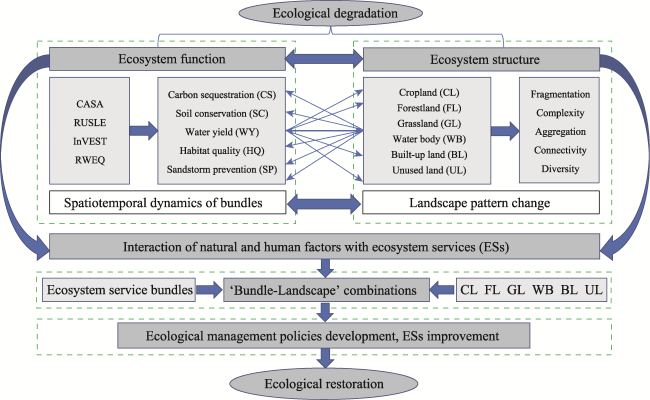
Figure 1 Study flowchart |
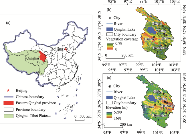
Figure 2 Geographical location (a), vegetation coverage (b), and elevation (c) of the eastern Qinghai province |
Table 1 Multiple source datasets |
| Data type | Specific data | Time resolution | Spatial resolution | Data sources |
|---|---|---|---|---|
| Meteorological data Soil data | Precipitation, temperature, solar radiation, wind speed | day | — | China National Meteorological Science Data Center (http://data.cma.cn) |
| Actual evapotranspiration | year | 1 km | (https://doi.org/10.6084/m9.figshare.12278684.v5) from reference (Yin et al., 2021) | |
| Harmonized World Soil Database (HWSD) | — | 1 km | https://www.fao.org/ | |
| Vegetation data | Normalized vegetation dataset (NDVI) | month/year | 1 km | Resources and Environment Science and Data center, Chinese Academy of Sciences (http://www.resdc.cn/) |
| Topographic data | Digital elevation model (DEM) | — | 90 m | Geospatial Data Cloud (http://www.gscloud.cn/) |
| Socioeconomic data | Resident point Road network | — | — | Resources and Environment Science and Data center, Chinese Academy of Sciences (http:// www.resdc.cn/); OpenStreetMap (https:// download.geofabrik.de) |
| Other data | Long-term series of daily snow depth dataset in China | day | 25 km | National Qinghai-Tibet Plateau Scientific Data Center (http://data.tpdc.ac.cn/zh-hans/) |
| Land use and land cover data (LULC) | year | 1 km | Resources and Environment Science and Data Center, Chinese Academy of Sciences (http:// www.resdc.cn/) |
Table 2 Landscape pattern indices used in this study |
| Landscape indices | Indices description | Units | Range |
|---|---|---|---|
| Percentage of Landscape (PLAND) | Percentage of a certain landscape type in the total landscape area | Percentage | 0≤ PLAND ≤ 100 |
| Patch Density (PD) | Number of patches per unit area | Number per 100 ha | PD>0 |
| Mean Patch Area (AREA_MN) | Average area of each patch in the landscape or class | ha | AREA_MN>0 |
| Edge Density (ED) | Proportion of the sum lengths of all edge segments involving each patch type to the total landscape area | m per ha | ED≥0 |
| Area-Weighted Mean Shape Index (SHAPE_AM) | Sum of the average shape factor of each patch type multiplied by the weight of the patch area in the landscape area | Dimensionless | SHAPE_AM≥1 |
| Aggregation Index (AI) | Nonrandomness or aggregation degree of different patch types in the landscape | Percentage | 0≤ AI ≤ 100 |
| Contagion Index (CONTAG) | Agglomeration degree or extension trend of different patch types in the landscape | Percentage | 0< CONTAG ≤ 100 |
| Shannon’s Diversity Index (SHDI) | Probability and diversity of patch types in the landscape | Dimensionless | SHDI≥0 |
| Shannon’s Evenness Index (SHEI) | Distribution uniformity of each component in the landscape | Dimensionless | 0≤ SHEI ≤ 1 |
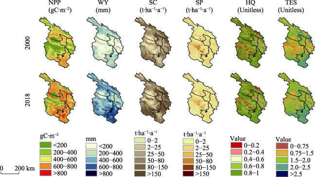
Figure 3 Spatiotemporal distribution of ESs in the eastern Qinghai province in 2000 and 2018 |
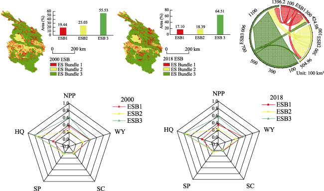
Figure 4 Spatiotemporal distribution and transfer of ecosystem service bundles in the eastern Qinghai province in 2000 and 2018 |
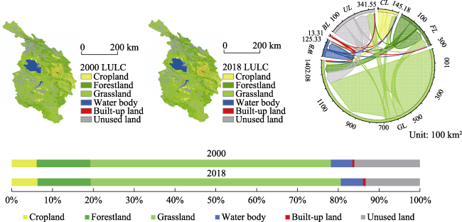
Figure 5 Spatiotemporal distribution and transfer of land use/land cover in the eastern Qinghai province in 2000 and 2018 |
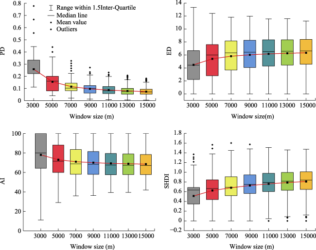
Figure 6 Boxplots of the landscape indices at the landscape scale |
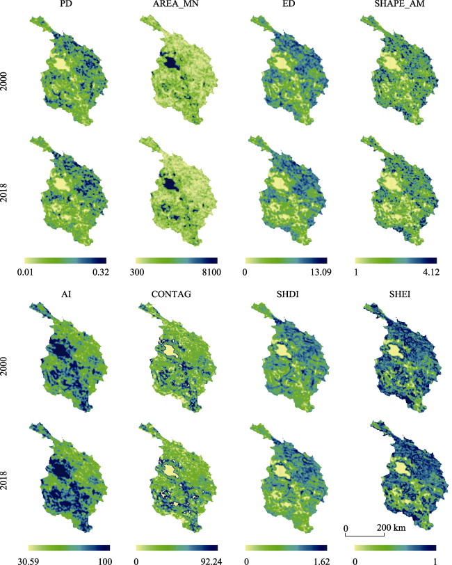
Figure 7 Spatiotemporal distribution of the landscape indices in the eastern Qinghai province in 2000 and 2018 |
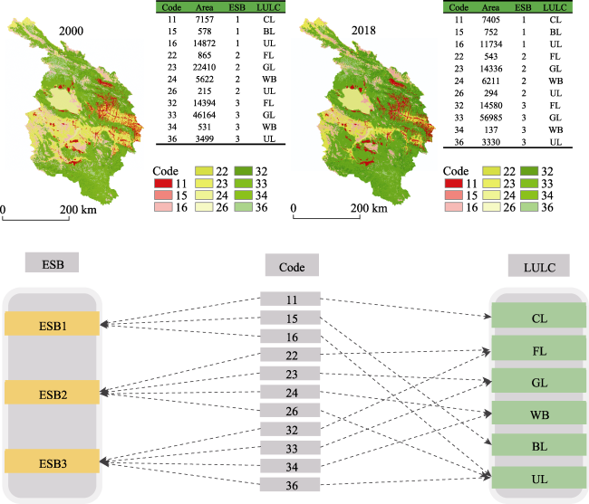
Figure 8 Spatial combinations of ‘bundle-landscape’ in the eastern Qinghai province in 2000 and 2018. Code refers to the code of the ‘bundle-landscape’ combination; Area is the area of each ‘bundle-landscape’ combination (km2); CL represents cropland; FL represents forestland; GL represents grassland; WB represents water body; BL represents built-up land; UL represents unused land. |
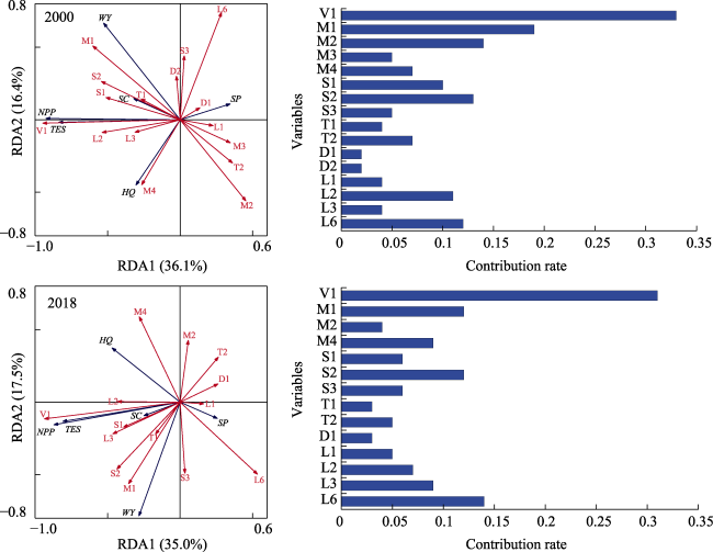
Figure 9 Redundancy analysis biplots and contribution rate of driving factors for the ESs in the eastern Qinghai province (Driving factors: V1, vegetation coverage; M1, precipitation; M2, temperature; M3, solar radiation; M4, actual evapotranspiration; S1, soil organic matter; S2, silt; S3, sand; T1, slope; T2, surface roughness; D1, distance from residential points; D2, distance from road; L1, percentage of cropland landscape; L2, percentage of forestland landscape; L3, percentage of grassland landscape; L6, percentage of unused land landscape) |
Table 3 Contribution rate of driving factors to changes in ESs in each ESB |
| ESBs | 2000ESB1 | 2000ESB2 | 2000ESB3 | 2018ESB1 | 2018ESB2 | 2018ESB3 | |
|---|---|---|---|---|---|---|---|
| Contribution rate of variables | V1 | 0.33 | 0.39 | 0.17 | 0.58 | 0.24 | 0.15 |
| M1 | 0.30 | 0.15 | 0.26 | 0.21 | 0.05 | 0.26 | |
| M2 | 0.36 | 0.10 | 0.17 | 0.33 | 0.01 | 0.08 | |
| M3 | 0.09 | 0.11 | 0.05 | 0.14 | 0.05 | 0.02 | |
| M4 | 0.24 | — | 0.11 | 0.23 | 0.37 | 0.12 | |
| M5 | — | 0.09 | 0.02 | 0.03 | 0.01 | ||
| S1 | 0.10 | 0.10 | 0.04 | 0.06 | 0.05 | 0.03 | |
| S2 | — | 0.25 | 0.01 | 0.12 | 0.24 | 0.04 | |
| S3 | 0.13 | 0.24 | 0.03 | 0.13 | 0.33 | 0.04 | |
| S4 | — | 0.19 | 0.03 | 0.16 | 0.22 | 0.03 | |
| T1 | 0.09 | 0.11 | 0.07 | 0.07 | 0.12 | 0.04 | |
| T2 | 0.13 | — | 0.08 | 0.05 | 0.19 | 0.06 | |
| D1 | — | 0.08 | — | 0.28 | 0.10 | 0.02 | |
| D2 | 0.16 | 0.05 | 0.03 | 0.23 | 0.03 | 0.03 | |
| L1 | 0.33 | — | — | 0.40 | — | — | |
| L2 | — | 0.04 | 0.09 | — | 0.02 | 0.08 | |
| L3 | — | 0.22 | 0.03 | — | 0.33 | 0.01 | |
| L4 | — | 0.35 | — | — | 0.42 | — | |
| L6 | 0.31 | — | 0.08 | 0.48 | 0.09 | 0.05 | |
Driving factors: V1, vegetation coverage; M1, precipitation; M2, temperature; M3, solar radiation; M4, actual evapotranspiration; M5, wind speed; S1, soil organic matter; S2, silt; S3, sand; S4, clay; T1, slope; T2, surface roughness; D1, distance from residential points; D2, distance from road; L1, percentage of cropland landscape; L2, percentage of forestland landscape; L3, percentage of grassland landscape; L4, percentage of water body landscape; L6, percentage of unused land landscape |
| [1] |
|
| [2] |
|
| [3] |
|
| [4] |
|
| [5] |
|
| [6] |
|
| [7] |
|
| [8] |
|
| [9] |
|
| [10] |
|
| [11] |
|
| [12] |
|
| [13] |
|
| [14] |
|
| [15] |
|
| [16] |
|
| [17] |
|
| [18] |
|
| [19] |
|
| [20] |
|
| [21] |
|
| [22] |
|
| [23] |
|
| [24] |
|
| [25] |
|
| [26] |
|
| [27] |
|
| [28] |
|
| [29] |
|
| [30] |
|
| [31] |
|
| [32] |
|
| [33] |
|
| [34] |
|
| [35] |
|
| [36] |
|
| [37] |
|
| [38] |
|
| [39] |
|
| [40] |
|
| [41] |
|
| [42] |
|
| [43] |
Millennium Ecosystem Assessment MEA, 2005. Ecosystems and Human Well-being:Synthesis. Washington, DC: Island Press.
|
| [44] |
|
| [45] |
|
| [46] |
|
| [47] |
|
| [48] |
|
| [49] |
|
| [50] |
|
| [51] |
|
| [52] |
|
| [53] |
|
| [54] |
|
| [55] |
|
| [56] |
|
| [57] |
|
| [58] |
|
| [59] |
|
| [60] |
|
| [61] |
|
| [62] |
|
| [63] |
|
| [64] |
|
| [65] |
|
| [66] |
|
| [67] |
|
| [68] |
|
| [69] |
|
| [70] |
|
| [71] |
|
| [72] |
|
| [73] |
|
| [74] |
|
| [75] |
|
| [76] |
|
| [77] |
|
| [78] |
|
| [79] |
|
| [80] |
|
/
| 〈 |
|
〉 |