Research Articles

Global and regional changes in working-age population exposure to heat extremes under climate change

  • CHEN Xi , 1 ,
  • LI Ning 2 ,
  • JIANG Dabang 1, 3
Expand
  • 1. National Institute of Natural Hazards, Ministry of Emergency Management of China, Beijing 100085, China
  • 2. School of National Safety and Emergency Management, Beijing Normal University, Beijing 100875, China
  • 3. Institute of Atmospheric Physics, CAS, Beijing 100029, China

Chen Xi (1993-), PhD, specialized in climate change impact assessment. E-mail:

Received date: 2022-10-17

  Accepted date: 2023-05-18

  Online published: 2023-10-08

Supported by

Research Grants from National Institute of Natural Hazards, Ministry of Emergency Management of China(ZDJ2021-15)

China Postdoctoral Science Foundation(2021M702771)

Abstract

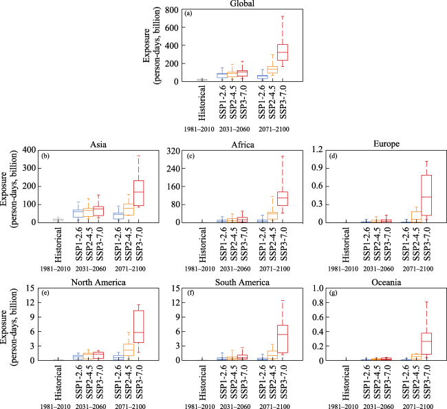
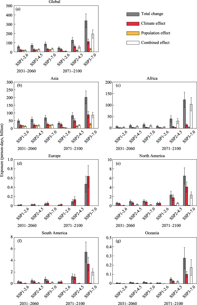
Despite recent progress in assessing future population exposure, few studies have focused on the exposure of certain vulnerable groups, such as working people. Working in hot environments can increase the heat-related risk to human health and reduce worker productivity, resulting in broad social and economic implications. Based on the daily climatic simulations from the Coupled Model Intercomparison Project phase 6 (CMIP6) and the age group-specific population projections, we investigate future changes in working-age population exposure to heat extremes under multiple scenarios at global and continental scales. Projections show little variability in exposure across scenarios by mid-century (2031-2060), whereas significantly greater increases occur under SSP3-7.0 for the late century (2071-2100) compared to lower-end emission scenarios. Global exposure is expected to increase approximately 2-fold, 6-fold and 16-fold relative to the historical time (1981-2010) under SSP1-2.6, SSP2-4.5 and SSP3-7.0, respectively. Asia will have the largest absolute exposure increase, while in relative terms, the most affected region is Africa. At the global level, future exposure increases are primarily caused by climate change and the combined effect of climate and working-age population changes. Climate change is the dominant driver in enhancing future continental exposure except in Africa, where the main contributor is the combined effect.

Cite this article

CHEN Xi , LI Ning , JIANG Dabang . Global and regional changes in working-age population exposure to heat extremes under climate change[J]. Journal of Geographical Sciences, 2023 , 33(9) : 1877 -1896 . DOI: 10.1007/s11442-023-2157-z

1 Introduction

There is an adverse impact of heat stress on human health, and extreme heat can lead to acute heat stroke, heat exhaustion, and worsens cardiovascular diseases (Kovats and Hajat, 2008; Venugopal et al., 2020). Considering only air temperature is not adequate for measuring heat stress, and high humidity can reduce the efficiency of evaporative cooling (i.e., sweating), leading to body heat accumulation and consequent human health risks (Mora et al., 2017; Buzan and Huber, 2020). Heat extremes in a warming climate have received much attention, and a growing body of work that additionally considers humidity indicates that the intensity, frequency, and duration of extreme heat events tend to increase over time in most regions of the world (Matthews et al., 2017; Lee and Min, 2018; Buzan and Huber, 2020; Chen et al., 2020b; Li et al., 2020a; Schwingshackl et al., 2021; Wang et al., 2021). Many studies have indicated increased mortality arising from heat extremes and have shown that the future risk of heat-induced mortality and morbidity could be notably raised (Phung et al., 2016; Chen et al., 2017; Mora et al., 2017; Ahmadalipour and Moradkhani, 2018). In addition to threatening human health, hot extremes have far-reaching influences on crop yield, worker productivity and the social economy (Dunne et al., 2013; Deryng et al., 2014; Orlov et al., 2020; Liu et al., 2021).
The impact of climatic extremes on human society depends not only on the severity of hazards but also on the population’s spatial distribution (exposure) and their vulnerability and adaptive capacity to hazards (Field et al., 2012). One previous study also showed that countries with higher risks of climatic hazards also have the largest populations or GDP (Shi et al., 2016). The prediction of changes in exposure to climatic extremes is a key aspect of understanding future vulnerability and in turn creating mitigation and adaptation measures (Jones et al., 2015). Many attempts have been made to quantify future changes in population exposure to extreme high temperature events under combined scenarios of climatic and socioeconomic conditions on global and regional scales (Liu et al., 2017; Mishra et al., 2017; Huang et al., 2018; Chen et al., 2020a; Iyakaremye et al., 2021; Sun et al., 2021; Sun et al., 2022; Ullah et al., 2022b; Xie et al., 2022). Recent studies have focused on exploring population exposure to the combination of extreme high temperature and humidity. For example, Coffel et al. (2018) projected that population exposure to wet-bulb temperatures exceeding recent deadly heat waves will increase by a factor of five to ten by 2070-2080 under the high emission scenario. Employing the heat index (HI) and wet-bulb globe temperature (WBGT) as a measure of heat stress, Matthews et al. (2017) and Li et al. (2020b) evaluated the global population exposed to heat-humidity extremes with various warming levels. In addition to estimating future changes in population exposure on a global scale, some work has focused on regional exposure variations. Based on combinations of multiple shared socioeconomic pathways and representative concentration pathways, future exposure to dangerous heat defined by apparent temperature in 173 African cities has been explored (Rohat et al., 2019a). Ullah et al. (2022a) investigated future heat stress using WBGT and the related socioeconomic exposure across South Asia as well as its four subregions. These studies highlight the importance of comprehensively understanding future changes in population exposure to hot extremes, which have major implications for evaluating future heat-related risk.
Despite recent progress in assessing future population exposure, researchers have paid little attention to the exposure of certain vulnerable groups. Recently, two studies have examined historical trends and future variations of exposure of populations over 65 years old to heatwaves (Chambers, 2020; Park and Jeong, 2022), but how the exposure of working population to heat extremes will change with global warming and demographic changes is still unknown. Note that negative impacts on human health are not only due to exposure to excessive heat but also related to physical activities in hot conditions because the metabolic heat inside the body can be raised by physical activities (Kjellstrom, 2016). Working in a hot environment can elevate the risk of heat-related illness and reduce human performance (Xiang et al., 2014). Accordingly, several studies have investigated the economic costs of heat-induced reductions in worker productivity and suggested that the economic losses over many regions worldwide may be substantial (Takakura et al., 2017; Xia et al., 2018; Chavaillaz et al., 2019; Knittel et al., 2020; Orlov et al., 2020). Based on the above premise, this work estimates future exposure changes of working people to heat extremes from the perspective of climate and/or working population. Due to the lack of spatially explicit working population projections, we utilize the projection of the working-age population as a replacement as a crucial step toward assessing the future impact of heat extremes on workers. Since exposure is driven by climatic and demographic conditions that will change over time (Jones et al., 2015), future variations in climate and socioeconomic development need to be considered for the projections of population exposure (Rohat et al., 2019b).
Given the above, this study examines future changes in working-age population exposure to heat extremes at both global and continental levels. Daily outputs from climate models participating in the Coupled Model Intercomparison Project phase 6 (CMIP6), as well as population data from the Shared Socioeconomic Pathways (SSPs) are employed. Variations in the working-age population and heat extremes are first analyzed. The exposure is then quantified in the historical period (1981-2010) and two future periods (T1: 2031-2060 and T2: 2071-2100). Finally, we conduct a quantitative analysis to identify the dominant drivers of future variations in exposure and the relative contribution of individual factors.

2 Materials and methods

2.1 Data sources

The calculation of the daily maximum WBGT (WBGTmax) is based on the daily maximum temperature (Tmax) and minimum relative humidity (RHmin), as RH is lowest at the time of Tmax during the diurnal cycle (Betts et al., 2013). Daily data are the outputs of historical and future simulations from 16 general circulation models (GCMs) participating in CMIP6 (Table 1; Eyring et al., 2016). Future scenarios under the framework of CMIP6 are the combinations of SSPs (Riahi et al., 2017) and representative concentration pathways (RCPs; van Vuuren et al., 2011). For example, the SSP1-2.6 refers to the combination of SSP1 and RCP2.6 scenarios, reflecting a sustainable socioeconomic development pathway combined with an estimated radiative forcing up to 2.6 W m-2 in 2100 (O’Neill et al., 2016; Riahi et al., 2017). In order to maintain consistency with working population data, model projections under SSP1-2.6, SSP2-4.5 and SSP3-7.0 are selected for this study. Only the first ensemble member (r1i1p1f1) of each GCM is adopted for analysis. These GCMs are selected because they can provide daily simulations of both Tmax and RHmin from the historical experiment and three future experiments. All outputs of the 16 models are resampled to a common 0.5° × 0.5° using bilinear interpolation.
Table 1 Overview of the 16 CMIP6 GCMs, with model names in bold denoting the 12 GCMs chosen for this study
Model name Center, country or union Horizontal resolution
ACCESS-CM2 CSIRO-BOM, Australia 192 × 144
ACCESS-ESM1-5 CSIRO-BOM, Australia 192 × 145
CanESM5 CCCma, Canada 128 × 64
CMCC-ESM2 CMCC, Italy 288 × 200
EC-Earth3 EC-Earth-Cons, Europe 512 × 256
EC-Earth3-Veg EC-Earth-Cons, Europe 512 × 256
EC-Earth3-Veg-LR EC-Earth-Cons, Europe 320 × 160
FGOALS-g3 CAS, China 180 × 80
INM-CM4-8 INM, Russia 180 × 120
INM-CM5-0 INM, Russia 180 × 120
IPSL-CM6A-LR IPSL, France 144 × 143
KACE-1-0-G NIMS-KMA, Republic of Korea 192 × 144
MIROC6 MIROC, Japan 256 × 128
MPI-ESM1-2-HR MPI-M, Germany 384 × 192
MPI-ESM1-2-LR MPI-M, Germany 192 × 96
MRI-ESM2-0 MRI, Japan 320 × 160
Hourly near-surface air temperature (t2m) and dew point temperature (d2m) from the ERA5 reanalysis dataset (Hersbach et al., 2020) as established by the European Centre for Medium-Range Weather Forecasts are utilized to validate the historical simulation between 1981 and 2010, with a horizontal resolution of 0.5° × 0.5°. Hourly RH is calculated by combining hourly t2m with d2m. Due to the unavailability of daily Tmax and RHmin from the ERA5 reanalysis, we calculate the hourly temperature for each hour of the day and take the maximum hourly T as the daily Tmax for that day. Accordingly, the daily RHmin is the hourly RH corresponding to the maximum hourly T of the day. The reanalysis data are regridded to the same grid of CMIP6 GCMs to facilitate spatial comparison.
The Wittgenstein Centre for Demography and Global Human Capital (http://dataexplorer.wittgensteincentre.org/wcde-v2/) provides a series of scenarios of future population and human capital in 201 countries and regions with a population of more than 100,000 people in 2015, including SSP1, SSP2, SSP3, SSP2-ZM (SSP2-zero migration) and SSP2-DM (SSP2-double migration). Population projections are differentiated by five-year age groups ranging from 0 to 4 years old through 95 to 99 years old, as well as the 100+ age group. Currently, data are at the national scale and five-year temporal resolution from 1950 until 2100, and the projections are based on 2015 The unit of the downloaded population data is thousand persons. Here the impact of human migration is not considered, and we only use age group-specific population projections under SSP1, SSP2 and SSP3 scenarios. More detailed information about this dataset can be found in Lutz et al. (2018).
Global spatially explicit population data provided by the Socioeconomic Data and Applications Center (SEDAC; Jones and O’Neill, 2016), with decadal intervals over 2010-2100 and high spatial resolution (0.125° × 0.125°), are also used to calculate the population weight of each global land grid. The population data in 2010 and during 2020-2100 under SSP1, SSP2 and SSP3 scenarios are aggregated to a 0.5° grid of CMIP6 GCMs. Note that this fine-scale population data refers to the total population of all age groups, and the comparison between the two sources of the population dataset is shown in Table 2.
Table 2 Basic information of two sources of population data used in this study
Demographic data by age group Spatially explicit population data
Data source WIC SEDAC
Age group Five-year age (from 0-4 to 95-99 and 100+) Total population of all ages
Temporal resolution 5 years 10 years
Spatial resolution National level 0.125° × 0.125°
Historical period 1950-2015 2010
Future period 2020-2100 under SSP1, SSP2 and SSP3 2020-2100 under five SSPs
Spatial range 201 countries and regions Global land grid points

2.2 Estimating working-age population

Work ability is closely related to a person’s age, and the upper-lower limit of working age varies across countries. According to the international general standard, people aged 15-64 are considered the working-age group. Therefore, we add up the total number of people aged 15-64 provided by WIC in each country, which is regarded as the working-age population. To match climate data to facilitate exposure calculation, the national-scale working-age population is downscaled to a 0.5° horizontal grid of CMIP6 models based on population weight at grid levels. More specifically, for one grid point in a certain country, its number of working-age people is estimated by multiplying the total working-age population in this country by its gridded population weight. Countries with areas smaller than a 0.5° grid size are excluded, and finally we calculate gridded working-age populations in 168 countries (43 in Asia, 52 in Africa, 37 in Europe, 16 in North America, 12 in South America and 8 in Oceania). The spatial map of the studied areas is shown in Figure 1.
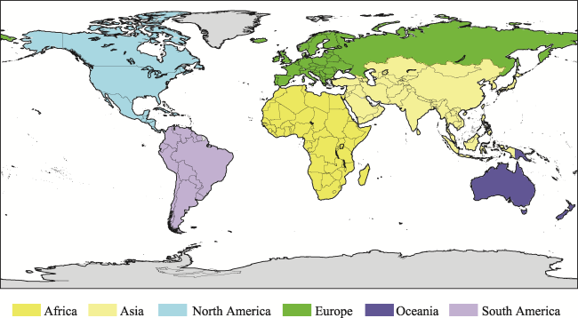
Figure 1 Spatial distribution of six continents consisting of 168 countries in this study

2.3 Calculating the wet-bulb globe temperature

Although there are many heat stress indicators (Buzan et al., 2015), WBGT is mostly used in assessing occupational health risks arising from extra heat in workplaces, as it has well validated thresholds related directly to various levels of physical activities (Willet and Sherwood, 2012). Following Tuholske et al. (2021), here the estimation of WBGT is based on the quantitative relationship between the heat index (HI) and WBGT (Bernard and Iheanacho, 2015). The calculation of daily maximum HI (HImax) follows the guidelines provided by the National Ocean and Atmospheric Administration:
H I max = c 1 + c 2 T max + c 3 R H min + c 4 T max R H min + c 5 T max 2 + c 6 R H min 2
+ c 7 T max 2 R H min + c 8 T max R H min 2 + c 9 T max 2 R H min 2
where Tmax is daily maximum temperature (°F), and RHmin is daily minimum relative humidity (%). c1 = -42.379; c2 = 2.04901523; c3 = 10.14333127; c4 = -0.22475541; c5 = -0.00683783; c6 = -0.05481717; c7 = 0.00122874; c8 = 0.00085282; c9 = -0.00000199.
If Tmax is between 80 and 112°F and RHmin is less than 13%, then the following adjustment needs to be subtracted from HImax:
A D J 1 = 13 R H min / 4 × 17 T max 95 / 17
If Tmax is between 80 and 87°F and RHmin is larger than 85%, then the following adjustment is added to HImax:
A D J 2 = R H min 85 / 10 × 87 T max / 5
If the calculated HImax is less than 80°F according to the above steps, then Steadman’s equation is used to compute daily HImax:
H I max = 0.5 × T max + 61 + 1.2 × T max 68 + 0.094 × R H min
We then convert daily HImax estimates to daily maximum WBGT (WBGTmax) using the following equation:
W B G T max = 0.0034 H I max 2 + 0.96 H I max 34
The unit of WBGTmax and HImax is °C and °F, respectively.

2.4 Identification of heat extremes

Instead of using the percentile-based threshold, here heat extremes are defined as daily WBGTmax exceeding an absolute threshold to provide consistent estimates of exposure that can be compared directly across the world. The International Standardization Organization (ISO) occupational heat stress standard provides reference limits of WBGT for the risk of heat-related diseases (Parsons, 2006). For example, for acclimatized humans with low and moderate metabolic rates, the reference WBGT is 30 and 28°C, respectively; for unacclimatized people at rest, the value is 32°C. Following Tuholske et al. (2021), we choose 30°C as the extreme heat threshold for WBGTmax that has been linked to greater death rates among vulnerable groups (Pradhan et al., 2019). As such, our heat threshold and exposure estimation are conservative.

2.5 Working-age population exposure to heat extremes

We adopt the method implemented by Jones et al. (2015) to calculate exposure, which is defined as the working-age population exposed to extreme heat. Exposure at each land grid is calculated by multiplying the number of downscaled working-age people by the annual total frequency of heat extremes (hereafter, referred to as HEF). Therefore, the unit of exposure is person-days. We calculate the 30-year average exposure for the 1981-2010, 2031-2060 (T1) and 2071-2100 (T2) periods using each model experiment, and the final results presented are the multimodel arithmetic mean. Such a multimodel ensemble method is necessary to assess the impact of climate change on thermal stress (Zhao et al., 2015). Moreover, we aggregate exposure on grid points to national, continental and global scales for further analysis.
To assess the individual effects of climate and working-age population, we decompose the population exposure change into three items: the climate effect, the working-age population effect, and their combined effect (Jones et al., 2015). We measure the former by holding the working-age population fixed at its historical level but allowing climate to change. The second is calculated as the exposure resulting from a changing working-age population under a constant climate. Their combined effect is equal to the total exposure change minus both the climate and population effects.

2.6 Evaluation of the CMIP6 general circulation models

The performance of the 16 CMIP6 GCMs in reproducing the historical annual HEF is evaluated by comparing the simulations with the ERA5 reanalysis. The geographical distribution of the averaged HEF over 1981-2010 simulated by each GCM is shown in Figure 2. We calculate the area mean bias and root-mean-square error (RMSE) for multimodel ensemble (MME) and each GCM (Figure 3). The results show that the annual HEF is well simulated by most CMIP6 models. The MME bias is 2.5 days, and its RMSE is 6.6 days. MIROC6 shows the lowest capacity in simulating the annual HEF, with a mean bias of 19.8 days and RMSE of 46.7 days. Based on the standard deviation and RMSE normalized against the reanalysis data, we choose relatively reliable GCMs. Finally, 12 models with normalized standard deviations and RMSEs less than 2.5 and 2, respectively, are regarded as good GCMs for reproducing historical annual HEF. The area mean bias and RMSE between the ensemble mean of these 12 GCMs and the reanalysis data are approximately 0.4 and 2.6 days, respectively, which are much smaller than the MME of 16 GCMs (Figure 3). Moreover, the historical annual HEF shows a similar spatial pattern with those in the ERA5 reanalysis, with higher values over some tropical regions in Africa, South America and Oceania (Figure 4). The spatial correlation coefficient between the historical annual HEF in the MME and ERA5 reanalysis data is 0.82, exceeding the 99% confidence level.
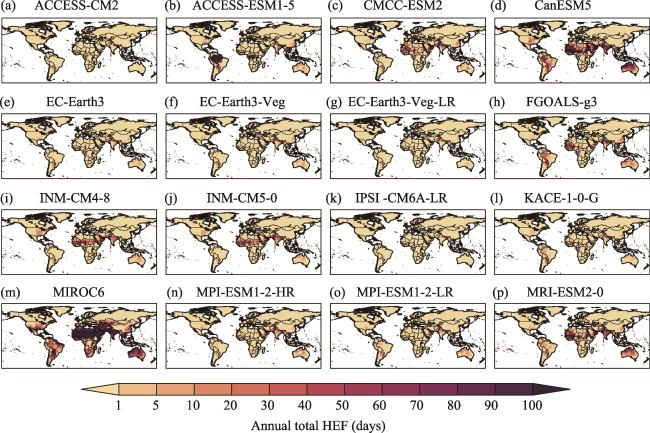
Figure 2 Geographical distributions of the simulated annual total HEF averaged over the historical period (1981-2010) for 16 CMIP6 GCMs
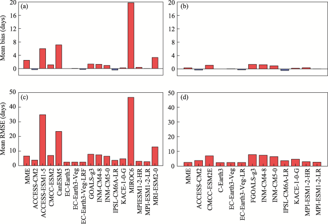
Figure 3 Global mean bias and RMSE for the annual total HEF during 1981-2010 for each CMIP6 model and MME in comparison with the ERA5 reanalysis
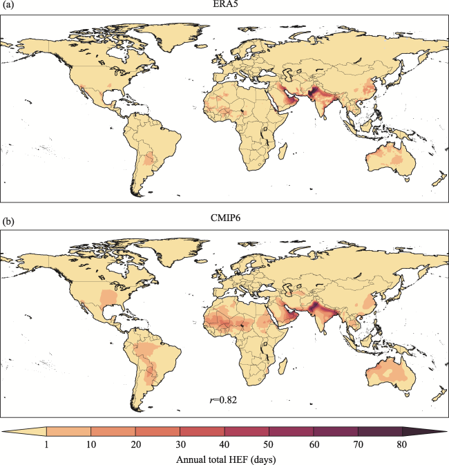
Figure 4 Spatial distributions of the annual total HEF averaged during 1981-2010 from the ERA5 reanalysis and MME of 12 CMIP6 models chosen for this study

Note: r is the spatial correlation coefficient between the MME and the reanalysis data, and it is statistically significant at the 99% confidence level.

3 Results

3.1 Working-age population projections

We analyze global and continental aggregate working-age population averaged over the historical period (1981-2010) and changes for the T2 period (2071-2100) under three SSP scenarios (Figure 5). In general, the number of working-age people has the largest increase under SSP3, followed by SSP2, and has the least increase with the SSP1 scenario. More specifically, the global aggregate annual working-age population for the historical period averages 3.7 billion, and in the T2 period, the increase is approximately 0.2, 1.8 and 4.2 billion under SSP1, SSP2 and SSP3, respectively. The future changes differ greatly across continents. During the historical period, the working-age population is the largest in Asia (nearly 2.3 billion) and the smallest in Oceania (less than 20 million). However, for the T2 period, Africa has the greatest increase especially under SSP3, with an increase of 5.7-fold relative to the historical level. Note that with the exception of Africa, continental aggregate changes in the working-age population tend to be negative under SSP1. Even under SSP3 representing a world with the highest population growth (Riahi et al., 2017), Europe is expected to have a negative increase in the number of working people.
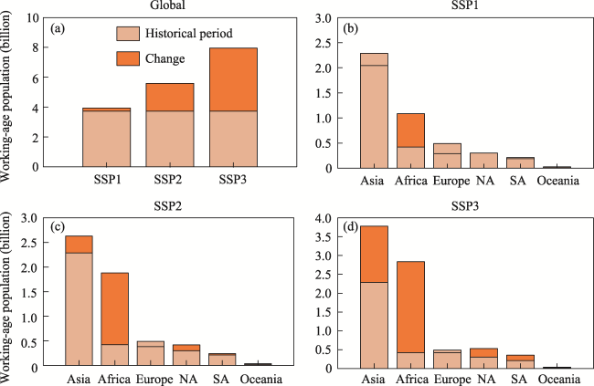
Figure 5 Global and continental aggregate working-age population in the historical period and future changes under three SSP scenarios (NA: North America, SA: South America)
Figure 6 illustrates the historical and projected changes in the working-age population in each continent and globally. The number of working-age people shows an upward trend over the historical period but displays different future changes across scenarios and continents. With the exception of Europe, where the working-age population will decline continuously, the population in other continents and the world will first increase until approximately the 2040s (2070s for Africa) and then decrease up to 2100 under SSP1 and SSP2. In contrast, the number of working-age people in most continents (except Europe) will continuously grow under the SSP3 scenario. The most rapid increase occurs in Africa, where the population will reach ~3 billion by 2100. For Europe, its working-age population will decrease until around the 2060s and increase afterward under SSP3.
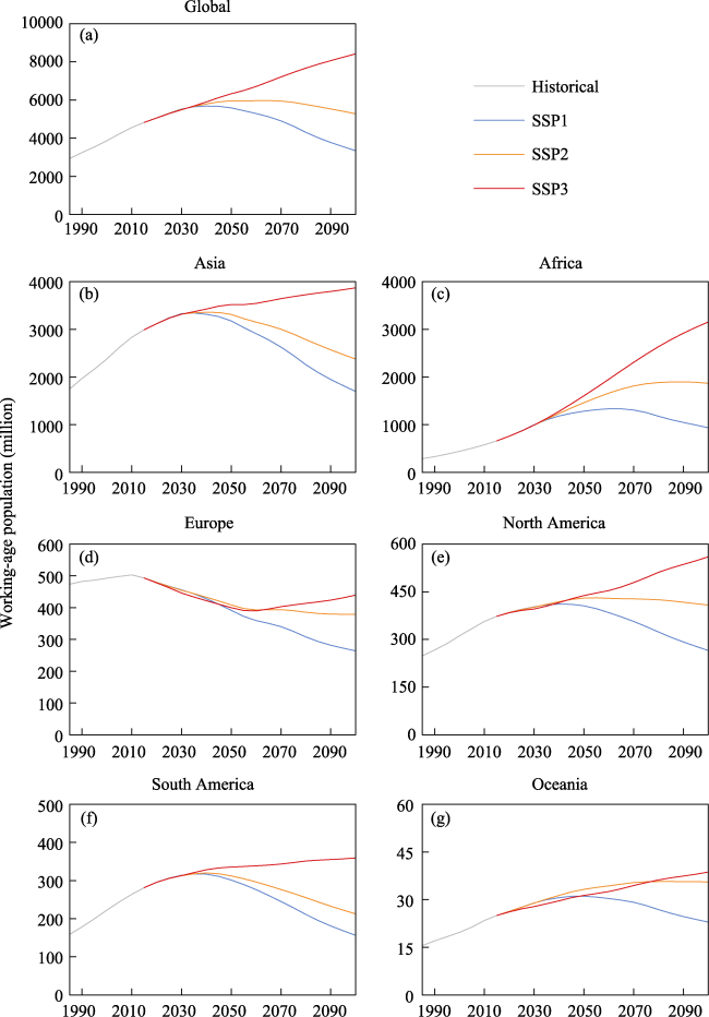
Figure 6 Time series of global and continental aggregate working-age population under three SSP scenarios

3.2 Heat extremes projections

Figure 7 displays the spatial patterns of the multimodel average HEF in the historical period and its future changes under three scenarios by comparing the annual HEF between 2071-2100 and 1981-2010. In the historical period, heat extremes rarely occur in most middle and high latitudes. In contrast, the annual total HEF in some tropical regions can exceed 10 or even 30 days. Future changes are relatively small at northern high latitudes, but the HEF increases substantially in the tropics and subtropics, especially under SSP3-7.0. For example, people living in the hottest regions in South America and North Africa will face extreme heat for almost half a year longer than in historical times. Under low and moderate emission scenarios, the largest increase in the annual HEF can also approach 49 and 107 days in some tropical regions, respectively. Our results demonstrate that the largest increases in the frequency of heat extremes occur in the tropics and subtropics, which agrees qualitatively with previous studies employing CMIP5 GCMs projections (Zhao et al., 2015; Matthews et al., 2017; Mora et al., 2017).
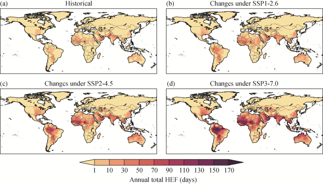
Figure 7 Geographical patterns of the annual total HEF averaged over the historical period and future changes averaged during 2071‒2100 relative to the historical level
We also calculate the number of countries that are unaffected by extreme heat and the number of countries with an average annual HEF above certain thresholds (30, 60 and 90 days) in both historical and two future periods (Figure 8). The number of countries without occurrence of heat extremes is 117 (interquartile range = 25) in the historical period, and it will decrease to 92 (32), 66 (26) and 45 (21) during 2071-2100 under SSP1-2.6, SSP2-4.5 and SSP3-7.0, respectively. In contrast, the number of countries experiencing heat extremes for more than 30, 60 and 90 days per year will rapidly increase for the T2 period under SSP3-7.0, approaching 40 (25), 25 (17) and 15 (11), respectively. It is also worth noting that during 2031-2060, differences in the number of countries suffering extreme heat are relatively small among various scenarios, whereas by the late century, lower emission scenarios substantially limit the occurrence of heat extremes compared to SSP3-7.0.
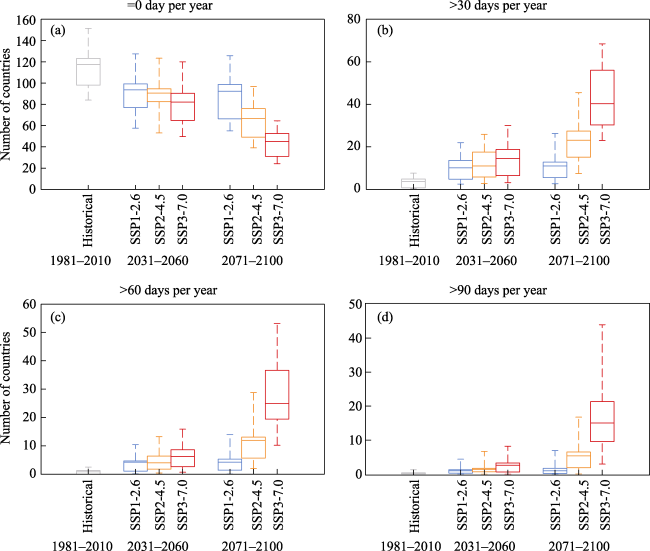
Figure 8 Projections of the number of countries without the occurrence of heat extremes and with an average HEF exceeding 30, 60 and 90 days per year. The boxplots indicate the spread of number of countries estimated from 12 CMIP6 GCMs, which represent uncertainties of climate model projections.

3.3 Future changes in exposure

Figure 9 shows the multimodel projections of global and continental aggregate working-age population exposure to heat extremes. During the historical period, global aggregate annual exposure averaged 18.9 (12.3) billion person-days. For the T1 period, it will increase under all three emission scenarios, and the differences in exposure among scenarios are small. Nevertheless, in the T2 period, the exposure under SSP3-7.0 is greater than that under the low and moderate emission scenarios. Global aggregate exposure increases roughly 2-fold, 6-fold and 16-fold compared to the historical level under SSP1-2.6, SSP2-4.5 and SSP3-7.0, respectively.
Figure 9 Projected global and continental aggregate exposure. The boxplots indicate the spread of exposure estimated from 12 CMIP6 GCMs, which represent uncertainties of climate model projections.
The historical exposure values are the highest in Asia (exceeding 16 billion person-days), followed by Africa (approximately 0.3 billion person-days), and the lowest in Europe (less than one million person-days). As expected, the smallest increase in exposure is seen under the combination of the low emission scenario (RCP2.6) and the socioeconomic scenario with slow population growth and low social vulnerability (SSP1), while the greatest increase holds under the relatively high emission scenario (RCP7.0) and the high population growth and vulnerability scenario (SSP3). Exposure projections at the continental scale also show little diversity across scenarios over the period of 2031-2060, compared to that over 2071-2100. For example, in Asia and Africa, the largest variability of exposure across scenarios for the T2 period is around 8.4 and 14 times greater than the T1 period. In the T2 period, due to a large growth in both working-age population and occurrences of heat extremes simultaneously, Asia is projected to have the most substantial increase in exposure, exceeding 152 billion person-days under SSP3-7.0. Conversely, Europe and Oceania are relatively unaffected, with a mean annual exposure of less than 0.5 billion person-days under all three scenarios. Although the absolute increase is smaller than that in Asia, models project that working-age population exposure in Africa increases by a factor of 363 relative to the historical period under SSP3-7.0. In addition, in North and South America, exposure is projected to increase by 47 and 159 times over historical levels, respectively.

3.4 Analysis of divers for exposure changes

We divide exposure changes into three components: the climate effect, the working-age population effect, and their combined effect. Figure 10 displays the increases in exposure and their components for two periods under three emission scenarios. The specific contribution rate of each factor to the total exposure change is given in Table 3. Globally, both the climate effect and the combined effect significantly account for the total exposure increase. Accordingly, the working-age population plays a relatively minor role under all scenarios, and its contribution decreases from T1 to T2. Under SSP1-2.6, the increase in total exposure mainly arises from climate change especially for the T2 period, with a contribution rate of 65%. In contrast, the climate effect becomes less important under SSP3-7.0, while the combined effect gets more important. During the T2 period, the contribution of the combined effect reaches up to 58%, with approximately 33% and 9% attributable to the effects of climate and working-age population, respectively. For the moderate emission scenario, the contribution rates from the climate effect and the combined effect are generally comparable. Taken together, climate change is the dominant factor driving enhanced exposure in the future, and the working-age population growth in hot regions also plays an important role under the relatively high emission scenario.
Figure 10 Multimodel average of global and continental aggregate changes in exposure and their components

Note: Error bars represent one standard deviation in projected exposure changes across the used models.

Table 3 Multimodel mean contribution rate of each factor to global and continental aggregate exposure changes (%)
Region Factor SSP1-2.6 SSP2-4.5 SSP3-7.0
T1 T2 T1 T2 T1 T2
Global Climate effect 39 65 36 47 36 33
Population effect 30 16 26 13 25 9
Combined effect 31 19 38 40 39 58
Asia Climate effect 40 74 38 60 39 44
Population effect 33 17 30 16 29 14
Combined effect 27 9 32 24 32 42
Africa Climate effect 25 27 21 17 20 12
Population effect 16 13 12 7 11 4
Combined effect 59 60 67 76 69 84
Europe Climate effect 100 100 100 100 100 100
Population effect 0 0 0 0 0 0
Combined effect 0 0 0 0 0 0
North America Climate effect 79 100 66 74 78 63
Population effect 5 0 4 2 3 1
Combined effect 16 0 30 24 19 36
South America Climate effect 71 100 68 94 64 62
Population effect 8 0 6 2 5 1
Combined effect 21 0 26 4 31 37
Oceania Climate effect 67 83 61 54 64 37
Population effect 10 4 6 2 2 0
Combined effect 23 13 33 44 34 63

Note: For regions in some cases with negative working-age population growth, the contribution rate for climate effect is set to 100%.

With the exception of Africa, the increase in total exposure aggregated at the continental scale is largely caused by the climate effect, particularly by the late 21st century under SSP1-2.6. In Africa, the combined effect is the dominant driver, and its role enlarges from the T1 to T2 period, resulting from the concurrent increase in heat extremes and working-age population. Under SSP3-7.0, the combined effect accounts for 69% and 84% of the total for the T1 and T2 periods, respectively. In Europe, where the working-age population is projected to decrease under all three SSPs, both the population effect and the combined effect tend to be negative such that the overall exposure change is less than that caused only by climate change. Similar to the globally aggregated results, the population effect plays a minor role in enhancing future exposure to heat extremes, with a contribution rate of less than ~15% across continents except Asia. In Asia, the population-induced exposure change accounts for approximately one-third of the total for the T1 period but is expected to decrease for the T2 period.

4 Discussion

Note that there exists uncertainty in assessing population exposure to climate change, owing mainly to the imperfection of climate models (Zhao et al., 2015; Jiang et al., 2016), the choice of emission scenarios (Fischer and Knutti, 2013), the population projection (Coffel et al., 2018; Rohat et al., 2019a), and the measure of climatic extremes (Liu et al., 2017). In this study, we account for the first two sources of uncertainty, and we try to reduce the model and scenario uncertainties by using the multimodel ensemble and three emission scenarios, respectively. The projection of the affected working-age population under climate change could depend on the definition of heat extremes. Instead of using percentile-based criteria to identify heat extremes, we employ an absolute impact-relevant threshold established in assessing occupational heat stress to provide a consistent estimation of exposure that can be compared directly across regions globally (Tuholske et al., 2021). Still, it is worth noting that the use of a globally uniform threshold does not account for the various acclimatization and vulnerability to heat stress in different regions of the world (Schwingshackl et al., 2021).
Several limitations to this study should be recognized. First, due to the lack of reliable labor force population data, we use the population projections differentiating age groups and calculate the number of working-age people. An important caveat is that our exposure does not represent the actual work force exposed to heat extremes. Rather, it refers to the exposure of the working-age population. In addition, future exposure changes are examined under three scenarios, and the relevant results under SSP5-8.5 are not explored in this study, as data from the population aged 15-64 with this scenario are not available. Second, the calculation of WBGT depends on the second order power relationship between HI and WBGT, and does not consider the effects of solar radiation and wind speeds. Also, our findings on heat extremes and exposure are determined by WBGTmax exceeding 30°C, which is the reference limit for acclimated people at low metabolic rates (Parsons, 2006) and is linked to increased mortality rates in workers (Pradhan et al., 2019). Quantitative analysis of exposure with other extreme heat event definitions needs to be conducted. Third, we adopt only a statistical method to downscale the age group-specific population projections at the national level, and the vulnerability and adaptation estimates are not considered. One of the primary impediments to integrating socioeconomic scenarios into risk assessments of climate extremes is the lack of geographically explicit projections of socioeconomic variables (Rohat et al., 2019b). Further studies are needed to include more accurate and high-resolution projections of demographic and socioeconomic conditions.

5 Conclusions

We investigate future changes in global and continental aggregate working-age population exposure to heat extremes defined by one day or longer periods when WBGTmax is above 30°C and assess the relative importance of climate and working-age population as drivers for the mid and late 21st century (T1: 2031-2060 and T2: 2071-2100) under three scenarios (SSP1-2.6, SSP2-4.5 and SSP3-7.0). It is found that the working-age population and its future changes vary largely across continents and scenarios. Asia has the largest working-age population in the historical period (1981-2010), and the most rapid increase is projected to occur in Africa. In general, the number of working-age people aggregated at the global and continental scales continuously decreases under SSP1 and SSP2, but increases under SSP3. The annual total frequency of heat extremes (HEF) is expected to increase substantially in the tropics and subtropics, particularly under SSP3-7.0, with an increase of ~6 months relative to the historical level in the hottest regions of South America and North Africa for the T2 period. Accordingly, the number of countries without the occurrence of heat extremes will rapidly decrease to 45 under SSP3-7.0, compared to 117 over the historical period. Moreover, differences in the number of countries suffering extreme heat are inconspicuous among the three scenarios during the T1 period compared to that in the T2 period.
At both global and continental scales, projections of working-age population exposure to heat extremes exhibit little variability across scenarios for the T1 period, but large increases in exposure occur under SSP3-7.0 for the T2 period compared to lower-end emission scenarios. By the late century, the global aggregate exposure is expected to increase approximately 2-fold, 6-fold and 16-fold relative to the historical level under SSP1-2.6, SSP2-4.5 and SSP3-7.0, respectively. Asia will face the largest absolute exposure increase, exceeding 152 billion person-days under SSP3-7.0, while Africa will have a striking 363-fold increase in exposure compared to the historical period. At the global level, future exposure increase is primarily driven by the climate effect and the combined effect, with the working-age population effect alone playing a relatively minor role especially for the T2 period. Among the six continents, the climate effect is the dominant driver in enhancing future exposure except in Africa which is largely caused by the combined effect. Under SSP3-7.0, the combined effect accounts for 69% and 84% of the total for the T1 and T2 periods, respectively. Overall, changes in the working-age population have limited influence on the continental exposure increase.
[1]
Ahmadalipour A, Moradkhani H, 2018. Escalating heat-stress mortality risk due to global warming in the Middle East and North Africa (MENA). Environment International, 117: 215-225.

DOI PMID

[2]
Bernard T E, Iheanacho I, 2015. Heat index and adjusted temperature as surrogates for wet bulb globe temperature to screen for occupational heat stress. Journal of Occupational and Environmental Hygiene, 12(5): 323-333.

DOI PMID

[3]
Betts A K, Desjardins R, Worth D, 2013. Cloud radiative forcing of the diurnal cycle climate of the Canadian prairies. Journal of Geophysical Research: Atmospheres, 118: 8935-8953.

[4]
Buzan J R, Huber M, 2020. Moist heat stress on a hotter earth. Annual Review of Earth and Planetary Sciences, 48(1): 623-655.

DOI

[5]
Buzan J R, Oleson K, Huber M, 2015. Implementation and comparison of a suite of heat stress metrics within the Community Land Model version 4.5. Geoscientific Model Development, 8(2): 151-170.

DOI

[6]
Chambers J, 2020. Global and cross-country analysis of exposure of vulnerable populations to heatwaves from 1980 to 2018. Climatic Change, 163(1): 539-558.

DOI

[7]
Chavaillaz Y, Roy P, Partanen A-I et al., 2019. Exposure to excessive heat and impacts on labour productivity linked to cumulative CO2 emissions. Scientific Reports, 9(1): 13711.

DOI PMID

[8]
Chen J, Liu Y, Pan T et al., 2020a. Global socioeconomic exposure of heat extremes under climate change. Journal of Cleaner Production, 277: 123275.

DOI

[9]
Chen K, Horton R M, Bader D A et al., 2017. Impact of climate change on heat-related mortality in Jiangsu province, China. Environmental Pollution, 224: 317-325.

DOI PMID

[10]
Chen X, Li N, Liu J et al., 2020b. Changes in global and regional characteristics of heat stress waves in the 21st century. Earth’s Future, 8: e2020EF001636.

[11]
Coffel E D, Horton R M, de Sherbinin A, 2018. Temperature and humidity based projections of a rapid rise in global heat stress exposure during the 21st century. Environmental Research Letters, 13(1): 014001.

DOI

[12]
Deryng D, Conway D, Ramankutty N et al., 2014. Global crop yield response to extreme heat stress under multiple climate change futures. Environmental Research Letters, 9(3): 034011.

DOI

[13]
Dunne J P, Stouffer R J, John J G, 2013. Reductions in labour capacity from heat stress under climate warming. Nature Climate Change, 3(6): 563-566.

DOI

[14]
Eyring V, Bony S, Meehl G A et al., 2016. Overview of the Coupled Model Intercomparison Project phase 6 (CMIP6) experimental design and organization. Geoscientific Model Development, 9(5): 1937-1958.

DOI

[15]
Field C B, Barros V, Stocker T F, 2012. Managing the Risks of Extreme Events and Disasters to Advance Climate Change Adaptation. A Special Report of Working Groups I and II of the Intergovernmental Panel on Climate Change. Cambridge: Cambridge University Press.

[16]
Fischer E M, Knutti R, 2013. Robust projections of combined humidity and temperature extremes. Nature Climate Change, 3(2): 126-130.

DOI

[17]
Hersbach H, Bell B, Berrisford P et al., 2020. The ERA5 global reanalysis. Quarterly Journal of the Royal Meteorological Society, 146(730): 1999-2049.

DOI

[18]
Huang D, Zhang L, Gao G et al., 2018. Projected changes in population exposure to extreme heat in China under a RCP8.5 scenario. Journal of Geographical Sciences, 28(10): 1371-1384.

DOI

[19]
Iyakaremye V, Zeng G, Yang X et al., 2021. Increased high-temperature extremes and associated population exposure in Africa by the mid-21st century. Science of The Total Environment, 790: 148162.

DOI

[20]
Jiang D B, Tian Z P, Lang X M, 2016. Reliability of climate models for China through the IPCC third to fifth assessment reports. International Journal of Climatology, 36(3): 1114-1133.

DOI

[21]
Jones B, O’Neill B C, 2016. Spatially explicit global population scenarios consistent with the shared socioeconomic pathways. Environmental Research Letters, 11(8): 084003.

DOI

[22]
Jones B, O’Neill B C, McDaniel L et al., 2015. Future population exposure to US heat extremes. Nature Climate Change, 5(7): 652-655.

[23]
Kjellstrom T, Briggs D, Freyberg C et al., 2016. Heat, human performance, and occupational health: A key issue for the assessment of global climate change impacts. Annual Review of Public Health, 37: 97-112.

DOI PMID

[24]
Knittel N, Jury M W, Bednar-Friedl B et al., 2020. A global analysis of heat-related labour productivity losses under climate change: Implications for Germany’s foreign trade. Climatic Change, 160(2): 251-269.

DOI

[25]
Kovats R S, Hajat S, 2008. Heat stress and public health: A critical review. Annual Review of Public Health, 29: 41-55.

PMID

[26]
Lee S-M, Min S-K, 2018. Heat stress changes over East Asia under 1.5°C and 2.0°C global warming targets. Journal of Climate, 31(7): 2819-2831.

DOI

[27]
Li C, Sun Y, Zwiers F et al., 2020a. Rapid warming in summer wet bulb globe temperature in China with human-induced climate change. Journal of Climate, 33(13): 5697-5711.

DOI

[28]
Li D, Yuan J, Kopp R E, 2020b. Escalating global exposure to compound heat-humidity extremes with warming. Environmental Research Letters, 15(6): 064003.

DOI

[29]
Liu Y, Zhang Z, Chen X et al., 2021. Assessment of the regional and sectoral economic impacts of heat-related changes in labor productivity under climate change in China. Earth’s Future, 9: e2021EF002028.

[30]
Liu Z, Anderson B, Yan K et al., 2017. Global and regional changes in exposure to extreme heat and the relative contributions of climate and population change. Scientific Reports, 7(1): 43909.

DOI

[31]
Lutz W, Goujon A, KC S et al., 2018. Demographic and Human Capital Scenarios for the 21st Century: 2018 Assessment for 201 Countries. Luxembourg: Publications Office of the European Union.

[32]
Matthews T K R, Wilby R L, Murphy C, 2017. Communicating the deadly consequences of global warming for human heat stress. Proceedings of the National Academy of Sciences of the United States of America, 114(15): 3861.

DOI PMID

[33]
Mishra V, Mukherjee S, Kumar R, 2017. Heat wave exposure in India in current, 1.5°C, and 2.0°C worlds. Environmental Research Letters, 12(12): 124012.

DOI

[34]
Mora C, Dousset B, Caldwell I R et al., 2017. Global risk of deadly heat. Nature Climate Change, 7(7): 501-506.

DOI

[35]
O’Neill B C, Tebaldi C, Van Vuuren D P et al., 2016. The scenario model intercomparison project (ScenarioMIP) for CMIP6. Geoscientific Model Development, 9(9): 3461-3482.

DOI

[36]
Orlov A, Sillmann J, Aunan K et al., 2020. Economic costs of heat-induced reductions in worker productivity due to global warming. Global Environmental Change, 63: 102087.

DOI

[37]
Park C-E, Jeong S, 2022. Population exposure projections to intensified summer heat. Earth’s Future, 10: e2021EF002602.

[38]
Parsons K, 2006. Heat stress standard ISO 7243 and its global application. Industrial Health, 44(3): 368-379.

[39]
Phung D, Thai P K, Guo Y et al., 2016. Ambient temperature and risk of cardiovascular hospitalization: An updated systematic review and meta-analysis. Science of The Total Environment, 550: 1084-1102.

DOI

[40]
Pradhan B, Kjellstrom T, Atar D et al., 2019. Heat stress impacts on cardiac mortality in Nepali migrant workers in Qatar. Cardiology, 143: 37-48.

DOI PMID

[41]
Riahi K, van Vuuren D P, Kriegler E et al., 2017. The shared socioeconomic pathways and their energy, land use, and greenhouse gas emissions implications: An overview. Global Environmental Change, 42: 153-168.

DOI

[42]
Rohat G, Flacke J, Dosio A et al., 2019a. Projections of human exposure to dangerous heat in African cities under multiple socioeconomic and climate scenarios. Earth’s Future, 7: 528-546.

DOI

[43]
Rohat G, Flacke J, Dosio A et al., 2019b. Influence of changes in socioeconomic and climatic conditions on future heat related health challenges in Europe. Global and Planetary Change, 172: 45-59.

DOI

[44]
Schwingshackl C, Sillmann J, Vicedo-Cabrera A M et al., 2021. Heat stress indicators in CMIP6: Estimating future trends and exceedances of impact-relevant thresholds. Earth’s Future, 9: e2020EF001885.

[45]
Shi P, Yang X, Fang J et al., 2016. Mapping and ranking global mortality, affected population and GDP loss risks for multiple climatic hazards. Journal of Geographical Sciences, 26(7): 878-888.

DOI

[46]
Sun S, Dai T, Wang Z et al., 2021. Projected increases in population exposure of daily climate extremes in eastern China by 2050. Advances in Climate Change Research, 12: 804-813.

DOI

[47]
Sun X, Ge F, Fan Y et al., 2022. Will population exposure to heat extremes intensify over Southeast Asia in a warmer world? Environmental Research Letters, 17(4): 044006.

DOI

[48]
Takakura Jy, Fujimori S, Takahashi K et al., 2017. Cost of preventing workplace heat-related illness through worker breaks and the benefit of climate-change mitigation. Environmental Research Letters, 12(6): 064010.

DOI

[49]
Tuholske C, Caylor K, Funk C et al., 2021. Global urban population exposure to extreme heat. Proceedings of the National Academy of Sciences of the United States of America, 118(41): e2024792118.

[50]
Ullah I, Saleem F, Iyakaremye V et al., 2022a. Projected changes in socioeconomic exposure to heatwaves in South Asia under changing climate. Earth’s Future, 10: e2021EF002240.

[51]
Ullah S, You Q, Chen D et al., 2022b. Future population exposure to daytime and nighttime heat waves in South Asia. Earth’s Future, 10: e2021EF002511.

[52]
van Vuuren D P, Edmonds J, Kainuma M et al., 2011. The representative concentration pathways: An overview. Climatic Change, 109(1): 5-31.

DOI

[53]
Venugopal V, Latha P K, Shanmugam R et al., 2020. Occupational heat stress induced health impacts: A cross-sectional study from South Indian working population. Advances in Climate Change Research, 11: 31-39.

DOI

[54]
Wang P, Yang Y, Tang J et al., 2021. Intensified humid heat events under global warming. Geophysical Research Letters, 48(2): e2020GL091462.

[55]
Willett K M, Sherwood S, 2012. Exceedance of heat index thresholds for 15 regions under a warming climate using the wet-bulb globe temperature. International Journal of Climatology, 32(2): 161-177.

DOI

[56]
Xia Y, Li Y, Guan D et al., 2018. Assessment of the economic impacts of heat waves: A case study of Nanjing, China. Journal of Cleaner Production, 171: 811-819.

DOI

[57]
Xiang J, Bi P, Pisaniello D et al., 2014. Health impacts of workplace heat exposure: An epidemiological review. Industrial Health, 52(2): 91-101.

DOI PMID

[58]
Xie W, Zhou B, Han Z et al., 2022. Substantial increase in daytime-nighttime compound heat waves and associated population exposure in China projected by the CMIP6 multimodel ensemble. Environmental Research Letters, 17: 045007.

DOI

[59]
Zhao Y, Ducharne A, Sultan B et al., 2015. Estimating heat stress from climate-based indicators: Present-day biases and future spreads in the CMIP5 global climate model ensemble. Environmental Research Letters, 10(8): 084013.

DOI

Outlines

/