
Journal of Geographical Sciences >
The impact of economic development on urban livability: Evidence from 40 large and medium-sized cities of China
|
Wang Yi (1989-), PhD and Associate Professor, specialized in human settlements and regional development. E-mail: wangyearn@163.com |
Received date: 2023-07-05
Accepted date: 2023-08-10
Online published: 2023-10-08
Supported by
National Natural Science Foundation of China(41901205)
Natural Science Foundation of Jiangsu Province(BK20190482)
Under the background that economy and urbanization of China are gradually entering the stage of high-quality development, clarifying the influence of economic development on urban livability is of significant academic and practical value. In this paper, regarded as one “factor”, livability was introduced into the research framework of production function, and a theoretical model of the impact of economic development on urban livability was established. Based on the panel data of 40 cities in China from 2005 to 2019, the System GMM, panel threshold model and other methods were further adopted to carry out an empirical analysis. The results show that: (1) The livability level of large and medium-sized cities in China from 2005 to 2019 has been rising generally, but they present obvious characteristics of dimensional and spatial differentiation. (2) In general, economic development has an inhibiting effect on the improvement of urban livability, but this logical effect shows obvious heterogeneity in different time periods and diverse city scales. This inhibitory effect is more significant for the cities before entering the new normal phase of economy, and large-scale municipalities and economically-developed provincial capitals (namely Class-A cities). (3) There are significant threshold effects in the impact of economic development on urban livability, where the threshold variables are income level and economic development. With the increase of city dwellers’ income, this effect presents an inverted N-shaped nonlinear feature. When the development of economy makes the average wage of employees between 60,000 and 80,000 yuan, economic development can significantly improve urban livability. Also, there is a significant single threshold inhibitory effect when economic development is taken as a threshold variable. However, its negative impact shows a law of diminishing marginal efficiency. In addition, a similar threshold effect is found in smaller-scale Class-B cities. The findings of this research can provide some insights for urban planners and policymakers in both China and vast developing countries to understand better the relationship between economic development and urban livability. Finally, according to the research findings, we proposed the corresponding policy enlightenment from both “macro guidance” and “micro action”.
WANG Yi , MIAO Zhuanying , LU Yuqi , ZHU Yingming . The impact of economic development on urban livability: Evidence from 40 large and medium-sized cities of China[J]. Journal of Geographical Sciences, 2023 , 33(9) : 1767 -1790 . DOI: 10.1007/s11442-023-2152-4
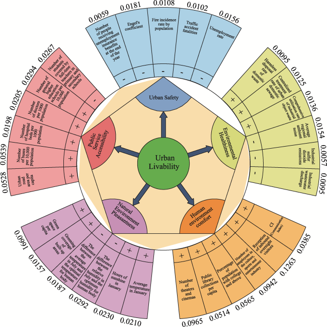
Figure 1 Evaluation index system diagram for urban livability |
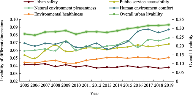
Figure 2 The change trend of the urban livability index from 2005 to 2019 in China |
Table 1 Descriptive statistics and validity tests |
| Variable | Definition | Observation | Mean | Std. dev | Minimum | Maximum | VIF | Fisher-PP |
|---|---|---|---|---|---|---|---|---|
| LnHB | Logarithm of urban livability | 600 | -1.430 | 0.324 | -2.241 | -0.353 | - | 100.06** (0.00) |
| LnEG | Logarithm of economic development | 600 | 17.887 | 1.114 | 14.643 | 20.232 | 3.16 | 244.05*** (0.01) |
| L | Credit scale | 600 | 4.110 | 3.505 | 0.153 | 17.176 | 1.91 | 402.22*** (0.00) |
| SI | Science and technology level | 600 | 3.456 | 0.435 | 2.408 | 4.399 | 1.54 | 522.32*** (0.00) |
| DF | Difference in fiscal adequacy | 600 | -22.917 | 94.565 | -647.209 | 232.062 | 2.13 | 681.84*** (0.00) |
| DLnSU | Difference in logarithm of industrial structure | 600 | 0.037 | 0.109 | -0.341 | 0.429 | 2.59 | 510.32*** (0.00) |
| LnAG | Logarithm of the square of GDP per capita | 600 | 22.459 | 0.975 | 19.913 | 24.299 | 1.77 | 229.07*** (0.00) |
| LnOP | Logarithm of economic openness | 600 | -3.606 | 1.051 | -10.407 | -1.678 | 1.42 | 108.24*** (0.00) |
| LnHP | Logarithm of house price | 600 | 8.886 | 0.591 | 7.634 | 10.432 | 1.98 | 378.63*** (0.00) |
| LnIC | Logarithm of income level | 600 | 10.806 | 0.495 | 9.750 | 11.781 | 3.01 | 700.18*** (0.00) |
Note: Figures in () are the z-values of the coefficients. ***, **, and * denote significance at the 1%, 5%, and 10% levels, respectively. The same as in the following table. |
Table 2 The estimation results of System GMM |
| Variables | Dependent variable: Logarithm of urban livability (LnHB) | |||||
|---|---|---|---|---|---|---|
| Entire sample | Entire sample | Before entering the new normal (2005-2014) | After entering the new normal (2015-2019) | Class-A cities | Class-B cities | |
| Lagged LnHB | 0.403*** | 0.496*** | 0.279*** | 0.856*** | 1.499** | 0.425*** |
| LnEG | 0.019* | -0.104** | -0.043 | 0.028* | -1.378** | -0.093* |
| CS | 0.038** | 0.058* | 0.007 | 1.527* | 0.000 | |
| SI | 0.076* | 0.282** | 0.064* | 3.243** | -0.006* | |
| LnAG | 0.039* | -0.036 | 0.067 | 0.367 | 0.055* | |
| DF | -0.017* | -0.015 | -0.004 | -0.105** | -0.160 | |
| DLnSU | -0.148 | 0.295 | -2.239*** | -1.608 | -2.024 | |
| LnOP | 0.027 | -0.062 | 0.065* | 0.102** | -0.096 | |
| _cons | -0.924*** | -1.842*** | -1.549** | 2.158** | -29.931** | 0.206*** |
| AR(1) | 0.000 | 0.000 | 0.000 | 0.062 | 0.098 | 0.000 |
| AR(2) | 0.427 | 0.214 | 0.915 | 0.819 | 0.249 | 0.160 |
| Sargan Test | 410.000 | 447.910 | 262.240 | 27.940 | 139.350 | 316.74 |
| WALD Test | 10913.12*** | 9765.45*** | 1356.66*** | 5673.21** | 9938.45** | 2367.81*** |
| N | 600 | 600 | 400 | 200 | 195 | 405 |
Note: The values reported for AR(1) and AR(2) are the p-values for the null hypothesis of no one-order and second-order serial correlation the first-differenced residuals. |
Table 3 Results of threshold effect significance test for the entire sample |
| Models | F value | P value | Number of BS | 1% critical value | 5% critical value | 10% critical value | |
|---|---|---|---|---|---|---|---|
| IC | Single threshold | 23.95 | 0.059 | 500 | 51.126 | 41.890 | 37.518 |
| Double threshold | 30.52 | 0.064 | 500 | 38.026 | 31.572 | 27.692 | |
| Triple threshold | 10.42 | 0.898 | 500 | 59.890 | 46.987 | 41.628 | |
| HP | Single threshold | 9.86 | 0.198 | 500 | 16.863 | 14.236 | 11.820 |
| Double threshold | 3.88 | 0.946 | 500 | 16.834 | 14.887 | 13.033 | |
| Triple threshold | 3.70 | 0.966 | 500 | 24.954 | 19.860 | 16.208 | |
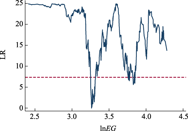
| EG | Single threshold | 25.96 | 0.036 | 500 | 28.962 | 24.857 | 21.545 |
| Double threshold | 9.27 | 0.290 | 500 | 18.330 | 14.137 | 12.624 | |
| Triple threshold | 6.88 | 0.952 | 500 | 37.812 | 31.348 | 28.071 | |
Table 4 Threshold regression results for the entire samples |
| Parameters | Estimated value | t statistic | Confidence interval |
|---|---|---|---|
| (1) α1: LnIC≤11.020 (IC ≤ 61083) | 0.088 | 1.25 | (-0.051, 0.226) |
| α2: 11.020 < LnIC≤11.367 (61083 < IC ≤ 86422) | 0.143** | 2.06 | (0.007, 0.280) |
| α3: 11.367 < LnIC (86422 < IC) | 0.073 | 1.09 | (-0.058, 0.204) |
| L | 0.208*** | 3.90 | (0.103, 0.313) |
| DLnSU | -0.131 | -1.46 | (-0.308, 0.045) |
| LnAG | -0.117*** | -3.50 | (-0.183, -0.051) |
| LnOP | 0.031 | 0.62 | (-0.052, 0.103) |
| SI | 0.012* | 1.21 | (0.098, 0.121) |
| DF | 0.022 | 0.69 | (-0.041, 0.085) |
| _cons | 0.338 | 0.57 | (-0.836, 1.513) |
| R2 | 0.465 | ||
| F statistic | 6.54 | ||
| (2) α1: LnEG ≤ 3.269 (EG ≤ 26.285) | -0.182** | -2.51 | (-0.324, -0.039) |
| α2: 3.269 < LnHP (EG >26.285) | -0.129* | -1.88 | (-0.264, 0.006) |
| L | 0.313*** | 5.79 | (0.207, 0.419) |
| DLnSU | -0.104 | -1.18 | (-0.278, 0.070) |
| LnAG | -0.134*** | -4.23 | (-0.196, -0.072) |
| LnOP | -0.076 | -1.31 | (-0.042, 0.085) |
| SI | 0.128** | 2.52 | (0.227, 0.028) |
| DF | -0.012 | -1.15 | (-0.033, 0.009) |
| _cons | -0.403 | -0.75 | (-1.464, 0.658) |
| R2 | 0.680 | ||
| F statistic | 11.00 |
Note: The robust standard error calculation was adopted in this paper. In the threshold significance test, the number of Bootstrap is 500. The following table is the same. |
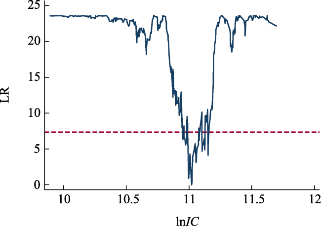
Figure 3 The first estimated threshold of income level in LR ( ) |
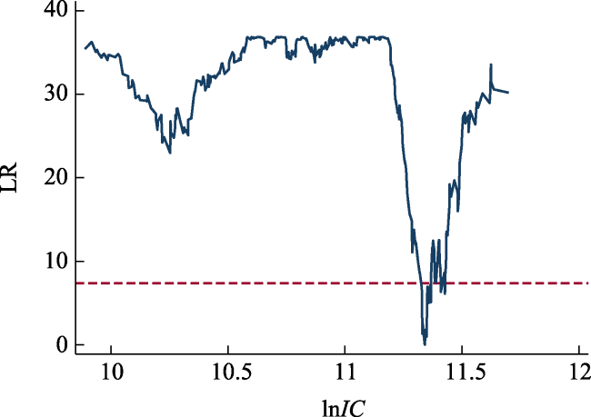
Figure 4 The second estimated threshold of income level in LR ( ) |
Figure 5 The estimated threshold of economic development in LR ( ) |
Table 5 Results of threshold effect significance test for diverse subsamples |
| Samples | Models | F value | P value | Number of BS | 1% critical value | 5% critical value | 10% critical value | |
|---|---|---|---|---|---|---|---|---|
| Class-A cities | IC | Single threshold | 9.14 | 0.590 | 500 | 26.722 | 22.267 | 20.022 |
| Double threshold | 5.72 | 0.698 | 500 | 24.147 | 19.132 | 15.890 | ||
| Triple threshold | 4.72 | 0.882 | 500 | 44.325 | 31.653 | 26.624 | ||
| EG | Single threshold | 8.95 | 0.304 | 500 | 20.653 | 15.632 | 13.278 | |
| Double threshold | 7.08 | 0.226 | 500 | 17.035 | 11.613 | 9.181 | ||
| Triple threshold | 2.74 | 0.884 | 500 | 32.327 | 18.646 | 15.122 | ||
| Class-B cities | IC | Single threshold | 30.86 | 0.039 | 500 | 51.653 | 44.924 | 39.519 |
| Double threshold | 43.1 | 0.000 | 500 | 31.309 | 23.745 | 21.317 | ||
| Triple threshold | 12.93 | 0.998 | 500 | 53.008 | 45.202 | 42.157 | ||
| EG | Single threshold | 21.55 | 0.034 | 500 | 25.015 | 20.541 | 18.838 | |
| Double threshold | 7.51 | 0.526 | 500 | 17.190 | 14.337 | 12.579 | ||
| Triple threshold | 8.17 | 0.986 | 500 | 37.026 | 32.045 | 30.118 | ||
Table 6 Threshold regression results for Class-B cities |
| Parameters | Estimated value | t statistic | Confidence interval |
|---|---|---|---|
| (1) α1: LnIC≤10.962 (IC≤57642) | 0.083 | 1.22 | (-0.052, 0.224) |
| α2: 10.962 < LnIC≤11.321 (57642<IC≤825) | 0.134** | 2.01 | (0.007, 0.282) |
| α3: 11.321 < LnIC (82573<IC) | 0.068 | 1.03 | (-0.056, 0.202) |
| L | 0.211*** | 3.94 | (0.106, 0.317) |
| DLnSU | -0.125 | -1.47 | (-0.303, 0.042) |
| LnAG | -0.117*** | -3.58 | (-0.181, -0.057) |
| LnOP | -0.058 | 0.93 | (0.154, 0.024) |
| SI | 0.014 | 0.23 | (-0.096, 0.124) |
| DF | 0.027 | 0.64 | (-0.042, 0.086) |
| _cons | 0.328 | 0.51 | (-0.833, 1.517) |
| R2 | 0.458 | ||
| F statistic | 6.51 | ||
| (2) α1: LnEG≤3.156 (EG≤23.476) | -0.202** | -2.34 | (-0.371, -0.032) |
| α2: 3.269 < LnEG (EG >23.476) | -0.146* | -1.78 | (-0.308, 0.015) |
| L | 0.287*** | 5.17 | (0.178, 0.396) |
| DLnSU | -0.147 | -1.56 | (-0.333, 0.039) |
| LnAG | -0.132*** | -3.66 | (-0.202, -0.061) |
| LnOP | -0.062 | 0.86 | (-0.141, -0.035) |
| SI | 0.100* | 1.72 | (0.115, 0.215) |
| DF | 0.014 | 0.40 | (-0.053, 0.080) |
| _cons | -1.787*** | -0.65 | (-1.676, -0.844) |
| R2 | 0.532 | ||
| F statistic | 6.18 |
| [1] |
|
| [2] |
|
| [3] |
|
| [4] |
|
| [5] |
|
| [6] |
|
| [7] |
|
| [8] |
|
| [9] |
|
| [10] |
|
| [11] |
|
| [12] |
|
| [13] |
|
| [14] |
|
| [15] |
|
| [16] |
|
| [17] |
|
| [18] |
|
| [19] |
|
| [20] |
|
| [21] |
|
| [22] |
|
| [23] |
|
| [24] |
|
| [25] |
|
| [26] |
|
| [27] |
|
| [28] |
|
| [29] |
|
| [30] |
|
| [31] |
|
| [32] |
|
| [33] |
|
| [34] |
|
| [35] |
|
| [36] |
|
| [37] |
|
| [38] |
|
| [39] |
|
| [40] |
|
| [41] |
|
| [42] |
|
| [43] |
|
| [44] |
|
| [45] |
|
| [46] |
|
| [47] |
|
| [48] |
|
| [49] |
|
| [50] |
|
| [51] |
|
| [52] |
|
| [53] |
|
| [54] |
|
| [55] |
|
| [56] |
|
| [57] |
|
| [58] |
|
| [59] |
|
| [60] |
|
| [61] |
|
| [62] |
|
| [63] |
|
| [64] |
|
| [65] |
|
/
| 〈 |
|
〉 |