Progress on spatial prediction methods for soil particle-size fractions

  • SHI Wenjiao , 1, 2, 3 ,
  • ZHANG Mo 1, 2, 3
Expand
  • 1. Key Laboratory of Land Surface Pattern and Simulation of CAS, Institute of Geographic Sciences and Natural Resources Research, CAS, Beijing 100101, China
  • 2. State Key Laboratory of Resources and Environmental Information System, Institute of Geographic Sciences and Natural Resources Research, CAS, Beijing 100101, China
  • 3. College of Resources and Environment, University of Chinese Academy of Sciences, Beijing 100049, China

Shi Wenjiao, PhD and Professor, geographic information analysis and remote sensing of resources and environment. E-mail:

Received date: 2023-05-19

  Accepted date: 2023-06-09

  Online published: 2023-07-24

Supported by

National Natural Science Foundation of China(41930647)

The Strategic Priority Research Program of the Chinese Academy of Sciences(XDA23100202)

The Strategic Priority Research Program of the Chinese Academy of Sciences(XDA20040301)

State Key Laboratory of Resources and Environmental Information System

Abstract

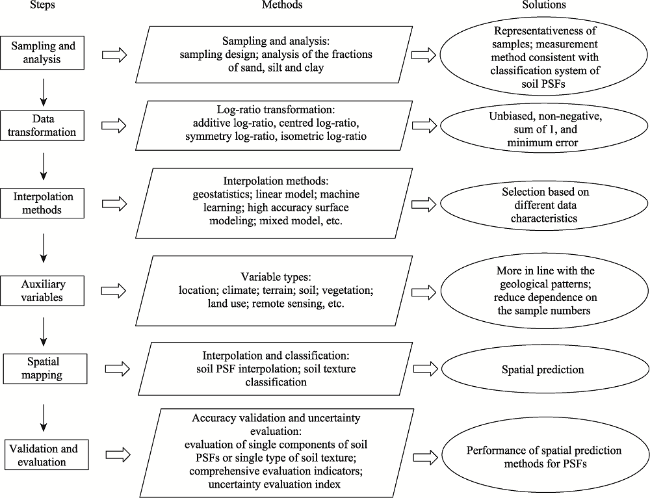
Soil particle-size fractions (PSFs), including three components of sand, silt, and clay, are very improtant for the simulation of land-surface process and the evaluation of ecosystem services. Accurate spatial prediction of soil PSFs can help better understand the simulation processes of these models. Because soil PSFs are compositional data, there are some special demands such as the constant sum (1 or 100%) in the interpolation process. In addition, the performance of spatial prediction methods can mostly affect the accuracy of the spatial distributions. Here, we proposed a framework for the spatial prediction of soil PSFs. It included log-ratio transformation methods of soil PSFs (additive log-ratio, centered log-ratio, symmetry log-ratio, and isometric log-ratio methods), interpolation methods (geostatistical methods, regression models, and machine learning models), validation methods (probability sampling, data splitting, and cross-validation) and indices of accuracy assessments in soil PSF interpolation and soil texture classification (rank correlation coefficient, mean error, root mean square error, mean absolute error, coefficient of determination, Aitchison distance, standardized residual sum of squares, overall accuracy, Kappa coefficient, and Precision-Recall curve) and uncertainty analysis indices (prediction and confidence intervals, standard deviation, and confusion index). Moreover, we summarized several paths on improving the accuracy of soil PSF interpolation, such as improving data distribution through effective data transformation, choosing appropriate prediction methods according to the data distribution, combining auxiliary variables to improve mapping accuracy and distribution rationality, improving interpolation accuracy using hybrid models, and developing multi-component joint models. In the future, we should pay more attention to the principles and mechanisms of data transformation, joint simulation models and high accuracy surface modeling methods for multi-components, as well as the combination of soil particle size curves with stochastic simulations. We proposed a clear framework for improving the performance of the prediction methods for soil PSFs, which can be referenced by other researchers in digital soil sciences.

Cite this article

SHI Wenjiao , ZHANG Mo . Progress on spatial prediction methods for soil particle-size fractions[J]. Journal of Geographical Sciences, 2023 , 33(7) : 1553 -1566 . DOI: 10.1007/s11442-023-2142-6

1 Introduction

Soil particle-size fractions (soil PSFs) are usually expressed as three components for discrete data—sand, silt, and clay. Most of soil physical and chemical characteristics and processes, such as soil moisture, heat and nutrient fluxes, soil composition and stability, as well as soil erosion, are affected by soil PSFs. Soil texture, which is composed of soil PSFs in different proportions, is one of the important attributes affecting soil physical, chemical and hydrological processes. Soil PSF interpolation and soil texture classification are key parameters of soil fertility management, ecosystem service assessment and hydrological models. Accurate spatial prediction of soil PSFs helps understand the simulation processes of these models.
Although soil researchers have reviewed on the digital soil mapping (Shi et al., 2012; Zhu et al., 2018; Zhang et al., 2020a), as compositional data, the spatial mapping of soil PSFs needs to meet the requirements of unbiased, non-negative, sum of 1 (100%) and minimum error (Odeh et al., 2003). The closure effect of soil PSFs shown in the soil texture triangle leads to pseudo-spatial correlation, which may make incorrect results if the statistical indicators in the Euclidean space are directly used (Filzmoser and Hron, 2009). Therefore, it is recommended to use the expression of the Aitchison space (i.e., Simplex) in the spatial prediction of soil PSFs (Aitchison, 1986). As soil PSF data have the characteristics of compositional data, data transformation should be firstly applied in the spatial interpolation, and the spatial prediction method should be chosen based on the data characteristics to meet those requirements and to obtain satisfactory interpolation accuracy and reasonable spatial distributions.
The methods for spatial prediction of soil PSFs involve a series of data transformation methods, different types of interpolation methods, validation of prediction accuracy and evaluation of uncertainty, and ways on improving the prediction accuracy. We reviewed the above issues to provide theory basis of the method selection for spatial prediction of soil PSFs, and also provided useful references for spatial prediction of other soil compositional data.

2 The framework of spatial prediction of soil PSFs

The spatial prediction of soil PSFs includes the sampling and analysis, the data transformation, the interpolation methods, combination of auxiliary variables, spatial mapping, accuracy validation and uncertainty evaluation (Figure 1).
Figure 1 The framework of spatial prediction methods for soil PSFs

2.1 Data transformation methods

There are four widely used types of data transformation methods for soil PSFs, including additive log-ratio (ALR) (Aitchison, 1986), centered log-ratio (CLR) (Aitchison, 1986), symmetry log-ratio (SLR) (Mcbratney et al., 1992; Odeh et al., 2003), and isometric log ratio (ILR) (Egozcue et al., 2003). Different log-ratio transformation methods have different formulas and performance. Some studies have systematically compared and analyzed log-ratio methods by combining them with interpolators, indicating that the ALR is asym-metric in Aitchison space (Wang and Shi, 2017, 2018; Zhang et al., 2020b). In addition, it is highly controversial due to the influence of subjective selection of denominators (Aitchison, 1986). The CLR is also not recommended. Although it is isometric, the sum of the numerator after the transformation is 1, resulting in a collinearity problem and singularity in the covariance matrix (Tolosana-Delgado et al., 2019). The ILR overcomes the above shortcomings. It eliminates model collinearity, and retains the advantages of isometry, scale invariance, and sub-component consistency (Egozcue et al., 2003; Filzmoser and Hron, 2009; Wang and Shi, 2018; Zhang et al., 2020b). Therefore, it has better performance in theory and application. Transformed and back-transformed equations for each method can be found in the reference of Wang and Shi (2017).

2.2 Interpolation methods

The commonly used interpolation methods for soil PSFs include geostatistics (Wang and Shi, 2018; Tolosana-Delgado et al., 2019), linear regression (Huang et al., 2014), machine learning (Zhang et al., 2020b) and so on.

2.2.1 Geostatistics

For the geostatistical methods, spatial prediction of soil PSFs used kriging methods combined with log-ratio transformations, such as log-ratio kriging (Wang and Shi, 2017, 2018), log-ratio cokriging (Tolosana-Delgado et al., 2019), and compositional kriging (CK) (De Gruijter et al. 1997; Taboada et al., 2013).
The geostatistical methods are widely used in spatial interpolation of soil attributes (Shi et al., 2005). Some soil researchers have applied ordinary kriging combined with log-ratio transformations for spatial interpolation of soil PSFs, and others have applied cokriging combined with log-ratio transformations. Both of them can generate satisfactory results (Lark and Bishop, 2007; Niang et al., 2014; Sun et al., 2014; Wang and Shi, 2017, 2018). On this basis, De Gruijter et al. (1997) proposed the CK method, which can simultaneously perform collaborative interpolation on different compositions (Walvoort and De Gruijter, 2001; Odeh et al., 2003). Some studies have improved the CK method and achieved better interpolation accuracy than the previous CK version (van den Boogaart and Tolosana-Delgado, 2008; Tolosana-Delgado and van den Boogaart, 2013). The prediction performance of CK has been proved to be relatively superior (Walvoort and De Gruijter, 2001; Zhang et al., 2011). In addition, both cokriging and CK involve cross-semivariance functions, in which standard variance estimation methods or robust variance estimation methods can be selected (Wang and Shi, 2018). The semivariance function in standard variance estimation is sensitive to outliers, which may overestimate the variance and increase interpolation error (Lark, 2000). To avoid this problem, Lark (2003) proposed robust variance estimation to improve the performance of the semi-variance, which was also confirmed later (Wang and Shi, 2018).

2.2.2 Linear regression

Multiple linear regression (MLR) is a widely used method for soil PSF interpolation, which is easy to express the relationship between soil attributes and environmental covariates, and has the advantages of strong interpretability (Buchanan et al., 2012). Remote sensing, terrain, vegetation and soil data can be combined with MLR as environmental covariates (Huang et al., 2014; Chagas et al., 2016). For spatial prediction of multi-layer soil PSFs, we can also explain various environmental covariates at different depths using MLR (Muzzamal et al., 2018). However, the use of traditional MLR is limited by the fact that the data should follow the normal distribution.
Compared to MLR, the stepwise regression model (SRM) can optimize models in environmental variables. The Akaike’s information criterion (AIC) is used to identify and eliminate redundant variables, and minimize the multicollinearity through statistical indicators and outlier. In spatial prediction of soil PSFs, some studies used MLR and further combined kriging method to improve the model accuracy (Vasques et al., 2016).
The generalized linear model (GLM) has been improved in the requirement of data distribution compared to MLR, which includes response variables with non-normal distribution (Nelder and Wedderburn, 1972). In addition, a link function has been embedded in GLM to connect independent and dependent variables, ensuring that the model meets the assumptions of linear regression. Note that if the link function is selected as Gaussian distribution, its result is completely equivalent to MLR (Nickel et al., 2014).
Generalized additive models (GAM) are extensions of GLM by introducing smoothing functions. GAM can model nonlinear relationships that are more complex than linear relationships derived from GLM (Buchanan et al., 2012). Moreover, the relationship between independent and dependent variables in GAM can be adjusted in a nonparametric method through a scatter graph smoother. Nonparametric regression widens the usual linear assumptions and can better reveal the relationship between independent and dependent variables (Mills et al., 2006).

2.2.3 Machine learning

Machine learning models can achieve both spatial interpolation of soil PSFs and spatial classification of soil texture (Hengl et al., 2015; Taalab et al., 2015; Zhang et al., 2020b). Previous studies found that machine learning models had better performance than linear models (e.g., MLR), showing more suitable prediction based on larger data sets (Hengl et al., 2015, 2017; Silva et al., 2020). However, different machine learning methods have different performance on soil PSF interpolation and soil texture classification. To systematically compare different machine learning methods, researchers compared K-nearest neighbor (KNN), multi-layer perceptron neural network (MLP), random forest (RF), support vector machine (SVM) and extreme gradient boosting (XGB) in the Heihe River Basin, China (Zhang et al., 2020b). They found that among the five machine learning models, tree models like RF and XGB performed better than KNN, MLP, and SVM. RF generated the best accuracy in both soil PSF interpolation and soil texture classification, but its computing time was relatively long. However, XGB predicted using parallel computing method, which is advantageous for processing large-scale data sets (Zhang et al., 2020b).

2.3 Accuracy validation and uncertainty evaluation

The accuracy validation and uncertainty evaluation of soil PSF are similar to other application in soil attributes (Zheng et al., 2003; Li et al., 2004; Lv et al., 2012; Zhang et al., 2020c), mainly include accuracy validation methods, accuracy validation indicators, and uncertainty evaluation indicators.

2.3.1 Accuracy validation methods

Probability sampling is a random sampling method based on classical sampling theory, which recollects new samples for accuracy validation through statistical inference based on design. It has been widely used for evaluating spatial prediction performance and mapping accuracy (Wadoux et al., 2021). Probability sampling has two characteristics. First, the probability of all samples being sampled in a population is positive. Second, the probability of being sampled is known (Wadoux et al., 2021). The most basic probability sampling is random sampling, i.e., the probability of all samples is equal. In addition, there are more complex probability sampling, such as hierarchical random sampling (De Gruijter et al., 2015), balanced sampling (Deville and Tillé, 2004; Brus, 2015), and local pivotal method (Grafström et al., 2012).
Researchers often use data splitting when the numbers of collected samples are limited. It divides data for both training and test, and the advantage is that no additional field sampling work is required (Lark and Bishop, 2007). Data splitting divides the original data sets into two subsets based on defined ratios, training dataset and test dataset (Silva et al., 2020). The training dataset is used for model training, and the test dataset is used for accuracy validation of interpolation results. Dataset can be divided into different proportions in terms of the size of the data, and the training dataset is typically randomly selected at a ratio of 70% to 90%. This process is generally repeated more than 30 times to ensure the reliability of validation results (Wang and Shi, 2017, 2018; Zhang et al., 2020b).
Cross validation, a typical form of data splitting, is a useful method for evaluating model performance, achieving reliable and unbiased results when applied to small datasets (Huang et al., 2014). Cross validation allows the data set to be divided into multiple training sets and test sets. The data is randomly divided into k groups. Each group is used in turn for validation, while the other k-1 groups are used for model training (Hengl et al., 2015). The types of cross validation include k-fold cross validation, leave-one-out cross validation (LOOCV), and nested cross validation. LOOCV may lead to high variance in estimation errors, so k-fold cross validation (e.g. 10-fold cross validation) is more popular (Huang et al., 2014). However, LOOCV is a better choice for some studies with limited numbers of soil samples.

2.3.2 Accuracy validation indicators

The accuracy validation of soil PSF interpolation can include the validation for each soil PSF component or soil texture type, comprehensive validation for multiple PSFs or texture types and so on. For soil PSFs, validation indicators for single component of PSFs include rank correlation coefficient (RCC), mean error (ME), root mean square error (RMSE), mean absolute error (MAE), and coefficient of determination (r2); comprehensive validation indicators include Aitchison distance (AD) and standardized residual sum of squares (STRESS). For soil texture types, validation indicators for single texture type include Precision-Recall curve, comprehensive indicators include overall accuracy and Kappa coefficient.
(1) Validation indicators for single component of soil PSF or texture type
The accuracy indicators for soil PSF interpolation include RCC, ME, RMSE, and r2. The equations are as follows:
$RCC=\frac{{{\sigma }_{Y{{Y}^{*}}\left( rank \right)}}}{{{\sigma }_{Y\left( rank \right)}}{{\sigma }_{{{Y}^{*}}\left( rank \right)}}}$
$ME=\frac{1}{n}\underset{i=1}{\overset{n}{\mathop \sum }}\,\left( {{Y}_{i}}-Y_{i}^{*} \right)$
$RMSE=\sqrt{\frac{1}{n}\underset{i=1}{\overset{n}{\mathop \sum }}\,{{\left( {{Y}_{i}}-Y_{i}^{*} \right)}^{2}}}$
${{r}^{2}}=1-\frac{\sum\limits_{i=1}^{n}{{{\left( Y_{i}^{*}-{{Y}_{i}} \right)}^{2}}}}{\sum\limits_{i=1}^{n}{{{\left( {{Y}_{i}}-{{{\bar{Y}}}_{i}} \right)}^{2}}}}$
where${{\sigma }_{Y\left( rank \right)}}$and${{\sigma }_{{{Y}^{*}}\left( rank \right)}}$are variances for observed and predicted values, respectively, and ${{\sigma }_{Y{{Y}^{*}}\left( rank \right)}}$is the covariance (Hengl et al., 2015). n is the number of observations (soil sampling points for validation). Yi is the observed value of the validation set, and Y*i is the predicted value of the validation set. ${{\bar{Y}}_{i}}$ is the mean of the observed values. ME measures prediction bias, and RMSE measures prediction accuracy. Higher RCC and r2, lower RMSE, and ME closer to 0 represent better model performance.
The accuracy indicators for the soil texture classification include Precision-Recall curves. The probabilities of different soil texture types (sum to 1) obtained during the training and predicting processes of machine learning models were selected to calculate the precision and recall, which indicated the extent of identifying positive cases:
$Recall=\frac{TP}{TP+FN}$
$Precision=\frac{TP}{TP+FP}$
where TP, FP and FN were true positive, false positive and false negative, respectively.
(2) Comprehensive evaluation indicators
For the comprehensive evaluation indicators of soil PSF interpolation accuracy, AD (Aitchison, 1990) and STRESS (Martin-Fernandez et al., 2001) showed the similarity between predicted and observed values, and the equations were as follows:
$AD=\sqrt{\underset{k=1}{\overset{D}{\mathop \sum }}\,{{\left( \ln \frac{Y}{{{\left( \mathop{\prod }_{k=1}^{D}Y \right)}^{\frac{1}{D}}}}-\ln \frac{{{Y}^{*}}}{{{\left( \mathop{\prod }_{k=1}^{D}{{Y}^{*}} \right)}^{\frac{1}{D}}}} \right)}^{2}}}$
$STRESS=\sqrt{\frac{\mathop{\sum }_{i<j}{{\left( A{{D}_{ij}}-AD_{ij}^{*} \right)}^{2}}}{\mathop{\sum }_{i<j}AD_{ij}^{2}}}$
where Yi is the observed value, and Y*i is the predicted value; D is the number of dimensions (for soil PSFs, D is 3); ADij and AD*ij are the ADs between the observed soil PSFs and the predicted soil PSFs at sites i and j.
For the comprehensive evaluation indicators of soil texture types, the overall accuracy is the number of samples of all correctly classified soil texture types divided by the total number of samples of soil texture types in validation sets; the Kappa coefficient represents the consistency between the observed and predicted classes, and the equations are as follows:
$Overall\ Accuracy=\frac{TP+TN}{TP+TN+FP+FN}$
$Kappa=\frac{{{p}_{o}}-{{p}_{e}}}{1-{{p}_{e}}}$
where TP, TN, FP and FN were true positive, true negative, false positive and false negative, respectively. po is the probability of observed agreement (overall accuracy), and pe is the probability of agreement when two classes are unconditionally independent. The ranges of these two indicators are from 0 to1, with higher values indicating better performance.

2.3.3 Uncertainty evaluation indicators

To provide accurate soil PSF prediction at a given location, the applicability indicators should also include the uncertainty of models (Vaysse and Lagacherie, 2017; Liu et al., 2020). Therefore, uncertainty evaluation is another perspective of the evaluation for soil PSF spatial prediction. The uncertainty evaluation indicators for soil PSF interpolation include prediction interval (PI), confidence interval (CI), and standard deviation (SD); the uncertainty evaluation indicators for soil texture classification include confusion index (COI), etc.
One of the commonly used methods for uncertainty evaluation is plotting the upper and lower limits of the 90% prediction interval (PI), i.e., there is a 90% probability that the true value range is between the upper and lower of the PI (Heuvelink, 2013). The PI equation is as follows (Liang et al., 2019):
$PI={{Y}^{*}}\pm 1.64\sqrt{MSE+{{\sigma }^{2}}}$
where Y*, MSE and σ2 are the mean, the mean square error of predicted values, and the variance from multiple validations, respectively, and 1.64 is the z-value corresponding to a 90% probability.
The CI can plus and minus 1.96 times of the standard errors (SE) from the predictions to obtain 95% of the upper and lower prediction limits, respectively. Its equation is as follows (Vitharana et al., 2019):
$CI={{Y}^{*}}\pm 1.96*PSE$
where Y* is the mean of the predicted values; PSE is the standard error of the residual prediction, and 1.96 is the z-value corresponding to a 95% probability.
In addition, the SD can be used as an indicator of model prediction uncertainty (Wang et al., 2017). It measures the degree to which a single point gathers around the average. The SD of validation indicators (such as RMSE) can reflect the uncertainty of the prediction (Liu et al., 2020). The equation of SD is as follows:
$SD=\sqrt{\frac{\mathop{\sum }^{}{{\left( {{Y}_{i}}-\bar{Y} \right)}^{2}}}{n-1}}$
where Yi is the value of the validation indicator at point i; $\bar{Y}~$is the mean value of validation indicator; n is the number of samples.
For the uncertainty evaluation of soil texture classification, models can be evaluated based on the COI of prediction probability (Zhang et al., 2020b), and the equation is shown as follows:
$COI=\frac{\mathop{\sum }_{i=1}^{n}\left[ 1-\left( {{P}_{max,i}}-{{P}_{secmax,i}} \right) \right]}{n}$
where Pmax,i is the highest probability value of soil sampling point i, Psecmax,i is the second highest probability value of soil sampling point i. Models with better performance will have lower COI.

3 Accuracy improvement of soil PSF interpolators

3.1 Improving data distribution through effective data transformation

Data transformation can make data follow normal distribution or be more symmetric, and can also effectively improve the prediction accuracy. Among the log-ratio transformations, the ILR method uses a sequential binary partition (SBP) for compositions, but selecting different SBPs would lead to different results (Zhang and Shi, 2020). Different permutations of components in compositional data can be used to establish ILR orthogonal systems through SBP, i.e., compositional balances (Tolosana-Delgado et al., 2019), which can form multiple sets of ILR data. Multiple compositional balances can lead to different covariance structures, demonstrating different results (Fiserova and Hron, 2011). However, studies of soil PSF interpolation have almost ignored this issue. Few researches compared different SBP options according to accurate evaluation, and analyzed whether these differences were caused by specific data sets or transformation methods. The selection of different SBPs can be based on prior expert knowledge, component biplot (Lloyd et al., 2012), variograms or cross variograms (Fiserova and Hron, 2011; Coenders et al., 2017; Facevicova et al., 2018; Molayemat et al., 2018) and so on. Some studies have used the highest percentage component of soil PSFs as the denominator in data transformation (Martins et al., 2016). However, if all of the three soil PSFs dominated the ILR components, the above methods cannot generate the best results (Tolosana-Delgado et al., 2005). Better performance was produced by using more symmetric ILR components in the SBP selection (Zhang and Shi, 2020). In addition, using log-ratio transformation before modeling could make it more difficult to interpret both trends and residuals. The optimal predicted value after log-ratio transformation may not be the optimal estimate after inverse.

3.2 Choosing appropriate prediction methods according to the data distribution

According to the characteristics of soil PSF data distribution, choosing appropriate spatial prediction methods can effectively improve the prediction accuracy. If data follow the normal distribution and have few outliers, the geostatistical model combined with the log-ratio transformation can reasonably produce the spatial patterns of soil PSFs (Wang and Shi, 2017). For the data with many outliers, using robust variance estimator in log-ratio cokriging method can significantly improve the mapping accuracy (Lark, 2000, 2003; Wang and Shi, 2018). For large-scale study areas with large variation of data sets and difficulty of sampling, such as basin scale (Zhang et al., 2020b), national scale (Akpa et al., 2014), and even global scale (Hengl et al., 2017), in which data always have strong spatial heterogeneity and relative non-normal distributions of sampling points. However, there are various types of environmental covariates. Therefore, methods such as machine learning combined with environmental covariates can be selected to modify the shortage of samples and data distributions.

3.3 Combining auxiliary variables to improve mapping accuracy and distribution rationality

Combining auxiliary variables (i.e., environmental covariates) is one of the important ways to improve the accuracy of soil PSF interpolation, especially for large-scale study areas (Zhang et al., 2020b). Auxiliary variables can be divided into continuous variables (such as elevation, normalized difference vegetation index, soil organic matter, soil bulk density, remote sensing data) and category variables (such as climate, topography, soil, vegetation, land use) (Odeh and Mcbratney, 2000; Buchanan et al., 2012; Akpa et al., 2014; Huang et al., 2014). Combining auxiliary variables can improve not only the accuracy of soil PSF interpolation, but also the rationality of spatial distribution of prediction maps, making more consistent with geological rules.

3.4 Improving interpolation accuracy using hybrid models

Spatial interpolation of soil PSF can use hybrid models to predict the trends and residuals, and then add them as the final prediction results. This hybrid model has been widely used in interpolation of soil properties (Hengl et al., 2004; Shi et al., 2011c; Keskin and Grunwald, 2018). Among them, trends can be predicted by linear regression or machine learning models combining with environmental covariates (Hengl et al., 2018), and the residuals can be predicted using ordinary kriging or high accuracy surface modeling (HASM) (Shi et al., 2011a; 2011b).
Other studies have combined Monte Carlo stochastic simulation with geostatistical model to predict soil particle size curves (PSC) (Menafoglio et al., 2014; Menafoglio et al., 2016b). This method uses the probability density function of soil PSF distribution, and treats these nonnegative and additive values as infinite compositional data, i.e., functional compositions. Compared to traditional methods, Monte Carlo stochastic simulation combined with geostatistics, Bayesian methods, and CLR transformation is more capable of depicting spatial variation and uncertainty of soil PSFs (Menafoglio et al., 2014; Menafoglio et al., 2016b).

3.5 Developing multi-component joint models

Most models predict each soil PSF component as a separate variable, ignoring the relationship among them, especially for log-ratio data. They cannot ensure that three components of back-transformed results are also optimal. It has been shown that using machine learning models (e.g., RF) combined with log-ratio transformed data may lead to biased estimates (Amirian-Chakan et al., 2019). To solve the above problems, it is necessary to develop a multi-component joint model.
Geostatistical models, such as compositional kriging, performs cross-covariance analysis for compositions of log-ratio transformed data, achieving spatial prediction of three soil PSFs. In regression models, Dirichlet regression is an available model for multi-component joint simulation (Hijazi and Jernigan, 2009). For machine learning methods, the multi-variate random forest is an extension of random forest, which can be used as a single model to predict all variables (Segal and Xiao, 2011), which can better consider the integrity of compositions, and generate more suitable in large study areas. Compared to current models that using discrete information from sand, silt, and clay, the Monte Carlo stochastic simulation has significant advantages in obtaining the integrity and continuity of data, making full use of its informative characteristics. Soil PSFs and soil textures can be extracted from the PSC results, achieving the purpose of spatial prediction (Menafoglio et al., 2016a; 2016b; Talská et al., 2018). In addition, HASM can also simulate three components simultaneously by solving equations in the model (Yue et al., 2007; 2016; 2020; Yue, 2011).

4 Conclusions

Based on the framework of spatial prediction method for soil PSFs, we systematically reviewed the research progress of spatial prediction method for soil SPFs from several aspects, such as data transformation method, selection of interpolation method, accuracy validation and uncertainty evaluation, and paths to improve the prediction accuracy of soil PSF. First, data transformation is an important way for the spatial prediction of soil PSFs, which is a key to make soil PSFs meet the requirements, and to improve the spatial prediction accuracy. Among several commonly used log-ratio transformation methods, the performance of ILR transformation is often better than others, so it is recommended in soil PSF interpolation. Secondly, for interpolation methods, we summarized the application and development of geostatistics, linear regression, and machine learning in soil PSF interpolation. Different interpolation methods have advantages and disadvantages, and researchers need to choose according to their needs. Thirdly, the accuracy validation and uncertainty evaluation of spatial prediction for soil PSFs are effective ways to distinguish the prediction performance of different models. We summarized the commonly used validation methods, and these indicators in soil PSF interpolation and soil texture classification. Fourthly, improving data distribution through effective data transformation, choosing appropriate prediction methods according to the data distribution, combining auxiliary variables to improve mapping accuracy and distribution rationality, improving interpolation accuracy using hybrid models, and developing multi-component joint models are effective ways to improve soil PSF prediction accuracy.
In the future, we should consider several perspectives of spatial prediction method of soil PSFs as follows: (1) using more effective data transformation methods to improve data distribution, and considering the principle and mechanism of data transformation; (2) developing multi-component joint models, such as Dirichlet regression, multivariate random forest model and high accuracy surface modeling, to improve prediction accuracy of soil PSFs; (3) introducing soil particle size curves and Monte Carlo stochastic simulation to enhance the integrity and continuity of prediction information, and extracting the soil PSFs information from these curves to realize spatial prediction.
[1]
Aitchison J, 1986. The Statistical Analysis of Compositional Data. London: Chapman and Hall.

[2]
Aitchison J, 1990. Measures of variability for geological data: Comment. Mathematical Geosciences, 22(2): 223-226.

[3]
Amirian-Chakan A, Minasny B, Taghizadeh-Mehrjardi R et al., 2019. Some practical aspects of predicting texture data in digital soil mapping. Soil and Tillage Research, 194: 104289.

[4]
Akpa S I C, Odeh I O A, Bishop T F A et al., 2014. Digital mapping of soil particle-size fractions for Nigeria. Soil Science Society of America Journal, 78(6): 1953-1966.

DOI

[5]
Brus D J, 2015. Balanced sampling: A versatile sampling approach for statistical soil surveys. Geoderma, 253/254: 111-121.

DOI

[6]
Buchanan S, Triantafilis J, Odeh I O A et al., 2012. Digital soil mapping of compositional particle-size fractions using proximal and remotely sensed ancillary data. Geophysics, 77(4): WB201-WB211.

DOI

[7]
Chagas C D, De Carvalho W, Bhering S B et al., 2016. Spatial prediction of soil surface texture in a semiarid region using random forest and multiple linear regressions. CATENA, 139: 232-240.

DOI

[8]
Coenders G, Martin-Fernandez J A, Ferrer-Rosell B, 2017. When relative and absolute information matter: Compositional predictor with a total in generalized linear models. Statistical Modelling, 17(6): 494-512.

DOI

[9]
De Gruijter J J, Minasny B, Mcbratney A B, 2015. Optimizing stratification and allocation for design-based estimation of spatial means using predictions with error. Journal of Survey Statistics and Methodology, 3(1): 19-42.

[10]
De Gruijter J J, Walvoort D J J, Van Gams P F M, 1997. Continuous soil maps: A fuzzy set approach to bridge the gap between aggregation levels of process and distribution models. Geoderma, 77(2): 169-195.

DOI

[11]
Deville J C, Tillé Y, 2004. Efficient balanced sampling: The cube method. Biometrika, 91(4): 893-912.

DOI

[12]
Egozcue J J, Pawlowsky-Glahn V, Mateu-Figueras G et al., 2003. Isometric logratio transformations for compositional data analysis. Mathematical Geosciences, 35(3): 279-300.

[13]
Facevicova K, Hron K, Todorov V et al., 2018. General approach to coordinate representation of compositional tables. Scandinavian Journal of Statistics, 45(4): 879-899.

DOI

[14]
Filzmoser P, Hron K, 2009. Correlation analysis for compositional data. Mathematical Geosciences, 41(8): 905-919.

DOI

[15]
Fiserova E, Hron K, 2011. On the interpretation of orthonormal coordinates for compositional data. Mathematical Geosciences, 43(4): 455-468.

DOI

[16]
Grafström A, Lundström N, Schelin L et al., 2012. Spatially balanced sampling through the pivotal method. Biometrics, 68(2): 514-520.

DOI PMID

[17]
Hengl T, De Jesus J M, Heuvelink G et al., 2017. SoilGrids250m: Global gridded soil information based on machine learning. PLOS ONE, 12(2): e0169748.

[18]
Hengl T, Heuvelink G, Kempen B et al., 2015. Mapping soil properties of Africa at 250 m resolution: Random forests significantly improve current predictions. PLOS ONE, 10(6): e0125814.

[19]
Hengl T, Heuvelink G, Stein A, 2004. A generic framework for spatial prediction of soil variables based on regression-kriging. Geoderma, 120(1/2): 75-93.

DOI

[20]
Hengl T, Nussbaum M, Wright M N et al., 2018. Random forest as a generic framework for predictive modeling of spatial and spatio-temporal variables. PeerJ, 6: 49.

[21]
Heuvelink G, 2013. Uncertainty quantification of GlobalSoilMap products. CRC Press-Taylor and Francis Group, 335-340.

[22]
Hijazi R, Jernigan R, 2009. Modelling compositional data using Dirichlet regression models. Journal of Applied Probability and Statistics, 4: 77-91.

[23]
Huang J, Subasinghe R, Triantafilis J, 2014. Mapping particle-size fractions as a composition using additive log-ratio transformation and ancillary data. Soil Science Society of America Journal, 78(6): 1967-1976.

DOI

[24]
Keskin H, Grunwald S, 2018. Regression kriging as a workhorse in the digital soil mapper’s toolbox. Geoderma, 326: 22-41.

DOI

[25]
Lark R M, 2000. A comparison of some robust estimators of the variogram for use in soil survey. European Journal of Soil Science, 51(1): 137-157.

DOI

[26]
Lark R M, 2003. Two robust estimators of the cross-variogram for multivariate geostatistical analysis of soil properties. European Journal of Soil Science, 54(1): 187-201.

DOI

[27]
Lark R M, Bishop T F A, 2007. Cokriging particle size fractions of the soil. European Journal of Soil Science, 58(3): 763-774.

DOI

[28]
Li X Y, Zhang S W, Wang Z M et al., 2004. Spatial variation and pattern analysis of soil properties in Dehui City of Jilin province. Acta Geographica Sinica, 59(6): 989-997. (in Chinese)

[29]
Liang Z Z, Chen S C, Yang Y Y et al., 2019. High-resolution three-dimensional mapping of soil organic carbon in China: Effects of Soilgrids products on national modeling. Science of the Total Environment, 685: 480-489.

DOI

[30]
Liu F, Zhang G L, Song X D et al., 2020. High-resolution and three-dimensional mapping of soil texture of China. Geoderma, 361: 114061.

[31]
Lloyd C D, Pawlowsky-Glahn V, Jose Egozcue J, 2012. Compositional data analysis in population studies. Annals of the Association of American Geographers, 102(6): 1251-1266.

DOI

[32]
Lv J S, Zhang Z L, Liu Y et al., 2012. Sources identification and hazardous risk delineation of heavy metals contamination in Rizhao city. Acta Geographica Sinica, 67(7): 971-984. (in Chinese)

DOI

[33]
Martins A B T, Bonat W H, Ribeiro P J, 2016. Likelihood analysis for a class of spatial geostatistical compositional models. Spatial Statistics, 17: 121-130.

DOI

[34]
Martin-Fernandez J A, Olea-Meneses R A, Pawlowsky-Glahn V, 2001. Criteria to compare estimation methods of regionalized compositions. Mathematical Geosciences, 33(8): 889-909.

[35]
Mcbratney A B, De Gruijter J J, Brus D J, 1992. Spatial prediction and mapping of continuous soil classes. Geoderma, 54(1): 39-64.

DOI

[36]
Menafoglio A, Guadagnini A, Secchi P, 2014. A kriging approach based on Aitchison geometry for the characterization of particle-size curves in heterogeneous aquifers. Stochastic Environmental Research and Risk Assessment, 28(7): 1835-1851.

DOI

[37]
Menafoglio A, Guadagnini A, Secchi P, 2016a. Stochastic simulation of soil particle-size curves in heterogeneous aquifer systems through a Bayes space approach. Water Resources Research, 52(8): 5708-5726.

DOI

[38]
Menafoglio A, Secchi P, Guadagnini A, 2016b. A class-kriging predictor for functional compositions with application to particle-size curves in heterogeneous aquifers. Mathematical Geosciences, 48(4): 463-485.

DOI

[39]
Mills A J, Fey M V, Grongroft A et al., 2006. Unravelling the effects of soil properties on water infiltration: Segmented quantile regression on a large data set from arid south-west Africa. Australian Journal of Soil Research, 44(8): 783-797.

[40]
Molayemat H, Torab F M, Pawlowsky-Glahn V et al., 2018. The impact of the compositional nature of data on coal reserve evaluation, a case study in Parvadeh IV coal deposit, Central Iran. International Journal of Coal Geology, 188: 94-111.

DOI

[41]
Muzzamal M, Huang J Y, Nielson R et al., 2018. Mapping soil particle-size fractions using additive log-ratio (ALR) and isometric log-ratio (ILR) transformations and proximally sensed ancillary data. Clays and Clay Minerals, 66(1): 9-27.

DOI

[42]
Nelder J A, Wedderburn R W M, 1972. Generalized linear models. Journal of the Royal Statistical Society: Series A (General), 135(3): 370-384.

[43]
Niang M A, Nolin M C, Jego G et al., 2014. Digital mapping of soil texture using RADARSAT-2 polarimetric synthetic aperture radar data. Soil Science Society of America Journal, 78(2): 673-684.

DOI

[44]
Nickel S, Hertel A, Pesch R et al., 2014. Modelling and mapping spatio-temporal trends of heavy metal accumulation in moss and natural surface soil monitored 1990-2010 throughout Norway by multivariate generalized linear models and geostatistics. Atmospheric Environment, 99: 85-93.

DOI

[45]
Odeh I O A, Mcbratney A B, 2000. Using AVHRR images for spatial prediction of clay content in the lower Namoi Valley of eastern Australia. Geoderma, 97(3/4): 237-254.

DOI

[46]
Odeh I O A, Todd A J, Triantafilis J, 2003. Spatial prediction of soil particle-size fractions as compositional data. Soil Science, 168(7): 501-515.

[47]
Segal M, Xiao Y Y, 2011. Multivariate random forests. Wiley Interdisciplinary Reviews: Data Mining and Knowledge Discovery, 1(1): 80-87.

[48]
Shi W J, Du Z P, Song Y J et al., 2011a. High accuracy surface modeling of soil properties based on multi-grid. Geographical Research, 30(5): 861-870. (in Chinese)

[49]
Shi W J, Liu J Y, Du Z P et al., 2011b. High accuracy surface modeling of soil properties based on geographic information. Acta Geographica Sinica, 66(11): 1574-1581. (in Chinese)

[50]
Shi W J, Liu J Y, Du Z P et al., 2011c. Surface modelling of soil properties based on land use information. Geoderma, 162(3/4): 347-357.

DOI

[51]
Shi W J, Yue T X, Shi X L et al., 2012. Research progress in soil property interpolators and their accuracy. Journal of Natural Resources, 27(1): 163-175. (in Chinese)

DOI

[52]
Shi Z, Jin H M, Li Y et al., 2005. Development and application of soft package for geostatistics. Journal of Soil and Water Conservation, (5): 172-175. (in Chinese)

[53]
Silva S H G, Weindorf D C, Pinto L C et al., 2020. Soil texture prediction in tropical soils: A portable X-ray fluorescence spectrometry approach. Geoderma, 362: 114136.

[54]
Sun X L, Wu Y J, Wang H L et al., 2014. Mapping soil particle size fractions using compositional kriging, cokriging and additive log-ratio cokriging in two case studies. Mathematical Geosciences, 46(4): 429-443.

DOI

[55]
Taalab K, Corstanje R, Zawadzka J et al., 2015. On the application of Bayesian networks in digital soil mapping. Geoderma, 259/260: 134-148.

DOI

[56]
Taboada J, Saavedra Á, Iglesias C et al., 2013. Estimating quartz reserves using compositional kriging. Abstract and Applied Analysis, 2013: 716593.

[57]
Talská R, Menafoglio A, Machalová J et al., 2018. Compositional regression with functional response. Computational Statistics & Data Analysis, 123: 66-85.

[58]
Tolosana-Delgado R, Mueller U, van den Boogaart K G, 2019. Geostatistics for compositional data: An overview. Mathematical Geosciences, 51(4): 485-526.

DOI

[59]
Tolosana-Delgado R, Otero N, Pawlowsky-Glahn V et al., 2005. Latent compositional factors in the Llobregat River Basin (Spain) hydrogeochemistry. Mathematical Geosciences, 37(7): 681-702.

[60]
Tolosana-Delgado R, van den Boogaart K G, 2013. Joint consistent mapping of high-dimensional geochemical surveys. Mathematical Geosciences, 45(8): 983-1004.

DOI

[61]
van den Boogaart K G, Tolosana-Delgado R, 2008. “Compositions”: A unified R package to analyze compositional data. Computers and Geosciences, 34(4): 320-338.

DOI

[62]
Vasques G M, Coelho M R, Dart R O et al., 2016. Mapping soil carbon, particle-size fractions, and water retention in tropical dry forest in Brazil. Pesquisa Agropecuaria Brasileira, 51(9): 1371-1385.

DOI

[63]
Vaysse K, Lagacherie P, 2017. Using quantile regression forest to estimate uncertainty of digital soil mapping products. Geoderma, 291: 55-64.

DOI

[64]
Vitharana U W A, Mishra U, Mapa R B, 2019. National soil organic carbon estimates can improve global estimates. Geoderma, 337: 55-64.

DOI

[65]
Wadoux A, Heuvelink G, Bruin S et al., 2021. Spatial cross-validation is not the right way to evaluate map accuracy. Ecological Modelling, 457: 109692.

[66]
Walvoort D J J, De Gruijter J J, 2001. Compositional kriging: A spatial interpolation method for compositional data. Mathematical Geosciences, 33(8): 951-966.

[67]
Wang S, Zhuang Q L, Wang Q B et al., 2017. Mapping stocks of soil organic carbon and soil total nitrogen in Liaoning province of China. Geoderma, 305: 250-263.

DOI

[68]
Wang Z, Shi W J, 2017. Mapping soil particle-size fractions: A comparison of compositional kriging and log-ratio kriging. Journal of Hydrology, 546: 526-541.

DOI

[69]
Wang Z, Shi W J, 2018. Robust variogram estimation combined with isometric log-ratio transformation for improved accuracy of soil particle-size fraction mapping. Geoderma, 324: 56-66.

DOI

[70]
Yue T X, 2011. Surface Modeling:High Accuracy and High Speed Methods. Boca Raton: CRC Press.

[71]
Yue T X, Du Z P, Song D J et al., 2007. A new method of surface modeling and its application to DEM construction. Geomorphology, 91(1): 161-172.

DOI

[72]
Yue T X, Liu Y, Zhao M et al., 2016. A fundamental theorem of Earth’s surface modelling. Environmental Earth Sciences, 75(9): 751.

DOI

[73]
Yue T X, Zhao N, Liu Y et al., 2020. A fundamental theorem for eco-environmental surface modelling and its applications. Science China-Earth Sciences, 63(8): 1092-1112.

DOI

[74]
Zhang G L, Shi Z, Zhu A X et al., 2020a. Progress and perspective of studies on soils in space and time. Acta Pedologica Sinica, 57(5): 1060-1070. (in Chinese)

[75]
Zhang J H, Li G D, Wang Y S et al., 2020c. Spatial characteristics and variation mechanism of different soil organic carbon components in the alluvial/sedimentaryzone of the Yellow River. Acta Geographica Sinica, 75(3): 558-570. (in Chinese)

[76]
Zhang M, Shi W J, 2020. Compositional balance should be considered in soil particle-size fractions mapping using hybrid interpolators. Hydrology and Earth System Sciences Discussions, https://doi.org/10.5194/hess-2020-384. [preprint]

[77]
Zhang M, Shi W J, Xu Z W, 2020b. Systematic comparison of five machine-learning models in classification and interpolation of soil particle size fractions using different transformed data. Hydrology and Earth System Sciences, 24(5): 2505-2526.

DOI

[78]
Zhang S W, Wang S T, Liu N et al., 2011. Comparison of spatial prediction method for soil texture. Transactions of the Chinese Society of Agricultural Engineering, 27(1): 332-339. (in Chinese)

[79]
Zheng Y M, Chen T B, Chen H et al., 2003. Spatial structure and distribution of Ni content in soil of suburbs of Beijing. Acta Geographica Sinica, 58(3): 470-476. (in Chinese)

[80]
Zhu A X, Yang L, Fan N Q et al., 2018. The review and outlook of digital soil mapping. Progress in Geography, 37(1): 66-78. (in Chinese)

DOI

Outlines

/