Research Articles

Investigating the critical influencing factors of snowmelt runoff and development of a mid-long term snowmelt runoff forecasting

  • ZHAO Hongling , 1, 2, 3 ,
  • LI Hongyan , 1, 2, 3, * ,
  • XUAN Yunqing 4 ,
  • BAO Shanshan 5 ,
  • CIDAN Yangzong 1, 2, 3 ,
  • LIU Yingying 1, 2, 3 ,
  • LI Changhai 1, 2, 3 ,
  • YAO Meichu 1, 2, 3
Expand
  • 1. College of New Energy and Environment, Jilin University, Changchun 130021, China
  • 2. Key Laboratory of Groundwater Resources and Environment, Ministry of Education, Jilin University, Changchun 130021, China
  • 3. Jilin Provincial Key Laboratory of Water Resources and Environment, Jilin University, Changchun 130021, China
  • 4. Department of Civil Engineering, Swansea University Bay Campus, Fabian Way, Swansea SA1 8EN, UK
  • 5. Yellow River Engineering Consulting Co. Ltd., Zhengzhou 450003, China
*Li Hongyan, Professor, specialized in hydrology and water resources. E-mail:

Zhao Hongling (1994-), PhD Candidate, specialized in hydrology and water resources. E-mail:

Received date: 2022-03-16

  Accepted date: 2022-12-27

  Online published: 2023-06-26

Supported by

The Key Program of National Natural Science Foundation of China(42230204)

Abstract

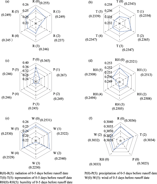
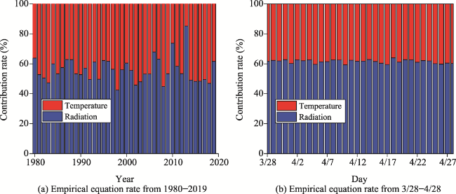
Snowmelt runoff is a vital source of fresh water in cold regions. Accurate snowmelt runoff forecasting is crucial in supporting the integrated management of water resources in these regions. However, the performances of such forecasts are often very low as they involve many meteorological factors and complex physical processes. Aiming to improve the understanding of these influencing factors on snowmelt runoff forecast, this study investigated the time lag of various meteorological factors before identifying the key factor in snowmelt processes. The results show that solar radiation, followed by temperature, are the two critical influencing factors with time lags being 0 and 2 days, respectively. This study further quantifies the effect of the two factors in terms of their contribution rate using a set of empirical equations developed. Their contribution rates as to yearly snowmelt runoff are found to be 56% and 44%, respectively. A mid-long term snowmelt forecasting model is developed using machine learning techniques and the identified most critical influencing factor with the biggest contribution rate. It is shown that forecasting based on Supporting Vector Regression (SVR) method can meet the requirements of forecast standards.

Cite this article

ZHAO Hongling , LI Hongyan , XUAN Yunqing , BAO Shanshan , CIDAN Yangzong , LIU Yingying , LI Changhai , YAO Meichu . Investigating the critical influencing factors of snowmelt runoff and development of a mid-long term snowmelt runoff forecasting[J]. Journal of Geographical Sciences, 2023 , 33(6) : 1313 -1333 . DOI: 10.1007/s11442-023-2131-9

1 Introduction

Snowmelt runoff is a vital recharge source of stream flow and groundwater (Barnett et al., 2005; Jenicek and Ledvinka, 2020), and in the meantime an essential component of water resources (Siderius et al., 2013; Li et al., 2021), supplying fresh water for around one billion people worldwide (Prestrud, 2007; Hock et al., 2010). Accurate and timely forecasting snowmelt runoff also plays an essential role in planning and allocating water resources (Li et al., 2013; Pyankov et al., 2018). However, snowmelt runoff processes often involve many meteorological factors and complex physical processes, which makes it very challenging to accurately simulate and further forecast snowmelt runoff (DeWalle and Rango, 2008; Bergström and Lindström, 2015).
For snowmelt forecasting, it is important to understand first the relationship between the meteorological influencing factors and snowmelt runoff before identifying the critical influencing ones (Vasil Ev et al., 2013). Common methods used in previous studies include, for instance, by analyzing the correlation coefficient between each factor and snowmelt runoff (Nabi et al., 2011; Zhang et al., 2014), or applying a local sensitivity analysis of individual factors (Zhang et al., 2016; Stigter et al., 2017; Zhang et al., 2022). However, these methods often failed to consider the joint effects of multiple factors. Moreover, they largely ignore the interactions among the meteorological factors on snowmelt runoff. These drawbacks inevitably affect the accuracy of identifying the critical influencing factors (Wang et al., 2013). Meanwhile, one must recognize that the effects of these meteorological factors are often associated with a time delay in terms of their contribution to the snowmelt process, i.e., time lags. For example, it has been found that the monthly average temperature has a one-month lag effect on the monthly snowmelt runoff in the Lijiang Basin (He et al., 2010). In the Amu Darya River Basin, the time lag of the precipitation conditions is particularly large, with a lag time ranging from 30 days to 90 days (Wang et al., 2021). Such lags, if not properly represented, can distort the relationship between the meteorological influencing factors and snowmelt runoff, hence introducing errors. How to investigate the critical influencing factors while considering the time lag effect and their interactions remains an important research question to address.
At present, forecasting of snowmelt runoff is primarily based on process-based hydrological models tailored to cold regions, such as HBV (Montero et al., 2016), SRM (Martinec et al., 2008; Xie et al., 2018), UBC (Hasson et al., 2019), CRHM (Pomeroy et al., 2007; Costa et al., 2020) and ARHYTHM (Zhang et al., 2000). However, the forecasting of the snowmelt runoff process generally has a short lead time. Therefore, it fails to forecast snowmelt runoff and meet the needs of flood and drought control. Accurate and timely mid-long term snowmelt runoff forecasting is vital for flood prevention and drought control.
Methods utilized in mid-long term snowmelt forecasting can be roughly classified into two types, i.e., time series analysis based methods and physical cause methods, depending on whether the physical influencing factors are considered. The time series analysis methods are data driven, and often have good adaptability in stable snowmelt runoff areas (Ouyang et al., 2010). However, these methods can face significant challenges when considering the impact of climate change that is manifested by the underlying climatology. The physical cause methods, in comparison, establish and employ the quantitative relationship between the early influencing factors and the later hydrological factors (Singh et al., 2000; Adnan et al., 2017). In recent years, nonlinear models that are based on artificial neural networks (ANN) and support vector regression (SVR) have been gradually applied to the field of mid-long term runoff forecasting (Xu et al., 2000; Corzo and Solomatine, 2007; Guo et al., 2011; Callegari et al., 2015; Feng et al., 2020).
Some studies have analyzed the relationship between meteorological factors and snowmelt runoff and further identified critical factors, however, interactions among the meteorological factors and their joint impacts on snowmelt runoff have not been well investigated. Moreover, the applicability of machine learning based methods in forecasting snowmelt runoff with a long lead time still needs to be explored. In this study, we systematically addressed both of these issues, by (i) firstly, investigating the critical influencing factors and their time lags using a global sensitivity analysis which can examine the effect of interactions among meteorological factors and their joint impacts; (ii) secondly, analyzing the correlation between the snowmelt runoff and influencing factors using a geostatistical analysis method; (iii) thirdly, establishing a set of empirical equations according to the correlation to calculate the contribution rate for seeking forecasting factor; (iv) finally, developing and validating an ANN and SVR based forecasting method for mid-long term snowmelt runoff forecasting with a month lead time using the identified influencing factor with biggest contribution rate.

2 Study area, data, and methods

2.1 Study area

Snowmelt runoff in China occurs primarily in several regions, including, the Northeast, accounting for 10%-25% of the total annual runoff (Li et al., 2019), the Eastern and Northern Inner Mongolia, the North and West of Xinjiang (11.2%) (Li et al., 2020), and Qinghai-Tibet Plateau area (34%) (Bookhagen and Burbank, 2010).
The study area discussed in this paper is the Baishan basin (roughly ranging between 126°28′-128°51′E and 41°42′-43°21′N) located in the mountainous plateau area of the cold region in Northeast China. The basin is the source area of the Second Songhua River, with elevations ranging from 3500 to 6400 m, and a total drainage area of 18,645.4 km2 (Figure 1). The Second Songhua River originates from the Changbaishan Tianchi and consists of two major tributaries: the Toudao Songhua river and the Erdao Songhua river. The area has a typical temperate continental monsoon climate, characterized by cold and long winters and rainy summers.
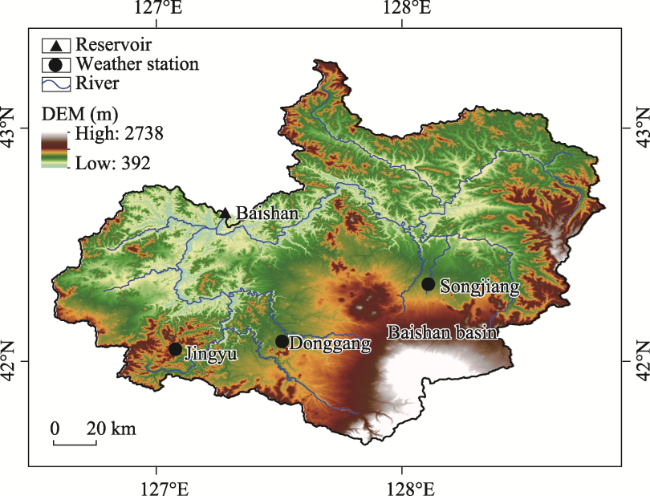
Figure 1 Location of the Baishan basin, river networks, gauging station, and weather stations
The annual average precipitation and temperature of the Baishan Basin are 750 mm and 4.3℃, respectively. Snow depth records for the period of April-November from 1980-2019 were used in this study. These data have been produced by using passive microwave remote sensing and supplied by the National Qinghai-Tibet Plateau Data Center (Che et al., 2008; Dai et al., 2015). The maximum snow depth over this period is 24.6 mm, and the average snow depth is 6.34 mm. Snowmelt runoff is found to occur mainly from 28 March to 28 April annually (Li et al., 2019) where the average annual snowmelt runoff accounts for 34.9% of total runoff in spring (Cidan et al., 2021). The most recent statistics (2018) show that the dominant land use is forest land (accounting for 88% of the study area), followed by farmland (7%) (Figure 2).
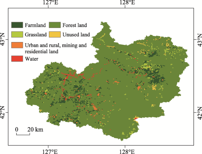
Figure 2 The land use of the Baishan basin

2.2 Data

Several types of data were utilized in this study. Firstly, gauged meteorological data of daily air temperature, daily precipitation (including rain and snow), and total solar radiation at three stations (Jingyu, Donggang, and Songjiang), including have been used in this study. They were provided by the National Meteorological Science Data Center (https://data.cma.cn). In addition, the global sunspot numbers from the World Sunspot Data Center (http://www.sidc.be/silso/datafiles) have also been also used. Secondly, cumulative snowfall was derived using the total precipitation at three meteorological stations from 1 November to 27 March of the following year (https://data.cma.cn). Thirdly, the study also uses the daily flow data from 28 March to 28 April 1980-2019 of the Baishan Reservoir, extracted from the 'Water Yearbook' published by the Baishan Power Plant of the Xinyuan Company of State Grid.
Snowmelt runoff in this study is identified as the flow from 28 March to 28 April because the seasonal permafrost period of the area is from October to April next year (Wang, 2010). Snowmelt runoff is treated as surface runoff, as groundwater recharge is small and stable in this area and rainfall is scarce from March to April.

2.3 Methods

The key methods employed in this study include global sensitivity analysis, geostatistical analysis, Back Propagation (BP) neural network algorithm, and Support Vector Regression (SVR). The work flow is divided into four steps (Figure 3):
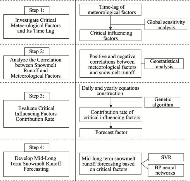
Figure 3 Flow chart describing the framework of the study
Step 1: a global sensitivity analysis based on BP neural networks (Li et al., 2012) was carried out to investigate the critical influencing meteorological factors and the time lag affecting the snowmelt runoff process. Considering the thermal components (temperature and solar radiation), moisture (humidity and precipitation), and air flow components (wind) affecting snowmelt runoff, daily total solar radiation, daily average wind speed, precipitation at 20-20 hours, relative humidity and daily average temperature are selected during snowmelt runoff period from 1980 to 2019.
Step 2: the correlation between the meteorological factors and snowmelt runoff is analyzed using the geostatistical analysis method (Sciarretta et al., 2001). The geostatistical analysis method can identify the positive and negative correlation between meteorological factors and snowmelt runoff.
Step 3: an empirical equation is derived based on the genetic algorithm (Chen et al., 1996). The equation is further used to quantitatively evaluate the contribution of the critical meteorological factors to snowmelt runoff for forecast factor selection.
Finally, after evaluating the contribution of the meteorological factors, the critical meteorological factor is identified as that comes with the most significant contribution rate for mid-long term snowmelt runoff forecasting. Once this is done, a mid-long term snowmelt runoff forecasting model is built using the BP neural network algorithm (Qu et al., 2003) and the SVR to represent the complex nonlinear relationship between the influencing factor and snowmelt runoff.

2.3.1 Global sensitivity analysis

For two related random variables X, the degree of the change of Y caused by the disturbance from X (the independent variable) is called the sensitivity of Y to X. Assuming a non-linear deterministic mapping relationship
Y = f ( X 1 , X 2 , , X i , , X n )
, the relationship can be summarized as follows:
y 1 = f ( x 1 , 1 , x 2 , 1 , , x i , 1 , , x n , 1 ) y 2 = f ( x 1 , 2 , x 2 , 2 , , x i , 2 , , x n , 2 ) y k = f ( x 1 , k , x 2 , k , , x i , k , , x n , k ) y m = f ( x 1 , m , x 2 , m , , x i , m , , x n , m )
where $m$ is the sample size; n is the independent variable dimension. For a change of xi,k+1 from its precedent value xi,k, i.e.,
x i , k + 1 = x i , k + Δ x i , k k + 1
, the corresponding change of yk+1 can be expressed as:
y k + 1 = y k + Δ y k k + 1 = f ( x 1 , k + Δ x 1 , k k + 1 , x 2 , k + Δ x 2 , k k + 1 , , x i , k + Δ x i , k k + 1 , , x n , k + Δ x n , k k + 1 )
According to the Taylor median theorem, Eq.(2) can be rewritten as:
f ( x 1 , k + Δ x 1 , k k + 1 , x 2 , k + Δ x 2 , k k + 1 , , x i , k + Δ x i , k k + 1 , , x n , k + Δ x n , k k + 1 ) f ( x 1 , k , x 2 , k , , x i , k , , x n , k ) + Δ x 1 , k k + 1 x 1 + Δ x 2 , k k + 1 x 2 + + Δ x i , k k + 1 x i + + Δ x n , k k + 1 x n x 1 , k , x 2. k , . . . , x i , k , . . . , x n , k + 1 2 ! Δ x 1 , k k + 1 x 1 + Δ x 2 , k k + 1 x 2 + + Δ x i , k k + 1 x i + + Δ x n , k k + 1 x n 2 x 1 , k , x 2 , k , . . . , x i , k , . . . , x n , k
Combining both Eqs.(2) and (3), it leads to:
Δ y k k + 1 = Δ x 1 , k k + 1 x 1 + Δ x 2 , k k + 1 x 2 + + Δ x i , k k + 1 x i + + Δ x n , k k + 1 x n x 1 , k , x 2 , k , . . . , x i , k , . . . , x n , k + 1 2 ! Δ x 1 , k k + 1 x 1 + Δ x 2 , k k + 1 x 2 + + Δ x i , k k + 1 x i + + Δ x n , k k + 1 x n 2 x 1 , k , x 2 , k , . . . , x i , k , . . . , x n , k
If we let
Δ y k k + 1 y k = η k
, then ηk is the mapping of the independent variable xi,k and its increment
Δ x i , k k + 1
, denoted as g(*).
η k = g ( x 1 , k , x 2 , k , , x i , k , , x n , k , Δ x 1 , k k + 1 , Δ x 2 , k k + 1 , , Δ x i , k k + 1 , , Δ x n , k k + 1 )
The mapping function $g(*)$ is fitted by using BP neural networks. $\Delta x_{i,k\to k+1}=0$ is introduced to calculate the influence of the increment of the independent variable on the dependent variable.
η i , k = g ( x 1 , k , x 2 , k , , x i , k , , x n , k , Δ x 1 , k k + 1 , Δ x 2 , k k + 1 , Δ x i - 1 , k k + 1 , 0 , Δ x i + 1 , k k + 1 , Δ x n , k k + 1 )
Therefore, the disturbance of dependent variables is $\beta_{i,k}=\eta_{i,k}-\eta^{'}_{i,k}$.
The overall disturbance effect of all samples is the sensitivity of the variable i:
${{\beta }_{i}}=\frac{\underset{k=1}{\overset{m}{\mathop{\mathop{\sum }^{}}}}\,\left| {{\beta }_{i,k}} \right|}{m}$

2.3.2 Geostatistical analysis

The geostatistical analysis method is used to study natural or social phenomena that are both spatially structural and random (Wheeler et al., 2013). This paper analyzes the correlation between snowmelt runoff and influencing factors by using the local polynomial interpolation (LPI) method of the geographic analysis module in ArcGIS software. The LPI method is a deterministic interpolation method that uses polynomials on all surfaces and has algorithmic functions corresponding to polynomial sequences (Wang et al., 2014).

2.3.3 Assessment of the contributions

Two forms of empirical equations (yearly and daily) were developed to quantify the effect of the main influencing factors, i.e., air temperature and solar radiation, on snowmelt runoff. The yearly model is aimed to account for the inter-annual variability. In contrast, the daily model attempts to reveal the relationship between the influencing factors and the snowmelt runoff at a daily time step. It should be noted that the daily model is fitted using the multi-year average data for each day, while the yearly model uses the annual data only. Unlike the yearly empirical equation, the daily scale equation needs to consider the time lag influence of temperature and wind speed on snowmelt runoff. The formula form mainly refers to the previous research results (Tian, 2019) and the correlation between snowmelt runoff and influencing factors.
The yearly model Eq.(8) shows the structure of the yearly model
Q ( y ) =   A S y x 1 * ( x 2 * S R y x 3 + x 4 * T y x 5 + x 6 *   W y x 7 +   x 8 * P y x 9 +   x 9 * H u y x 10 )
where Q(y) is runoff depth (mm), ASy is snow accumulation (mm), SRy is average total solar radiation in snowmelt runoff period (MJ/m2); Ty is the average temperature in snowmelt runoff period (°F); Wy is average wind speed (m/s) in snowmelt runoff period; Py is total precipitation during in snowmelt runoff period (mm); Huy is the average relative humidity in snowmelt runoff period (%). x1-x10 are optimized by genetic algorithm. Once calibrated, the equation becomes what is shown in Eq.(9):
Q ( y ) =   A S y 0.69 × ( - 0.3 S R y 0.83 - 0.33 T y 0.9 - 0.99 W y 0.41 +   0.72 P y 0.57 +   0.36 H u y 0.54 )
The daily model Eq.(10) shows the structure of the daily model:
Q ( i ) =   A S x 1 * ( x 2 * S r ( i ) x 3 + x 4 * T ( i - 2 ) x 5 + x 6 *   W ( i - 2 ) x 7 +   x 8 * P ( i ) x 9 +    x 9 * H u ( i ) x 10 )
where Q(i) is the daily runoff depth (mm) under annual average conditions, AS is the accumulated snow volume (mm), and Sr(i) is the mean annual daily total solar radiation (MJ/m2); T(i-2) is the temperature of the two days before the runoff date (°F); W(i-2) is the average wind speed of the previous two days of runoff date (m/s); P(i) is the mean annual daily precipitation (mm); Hu(i) is the mean annual daily relative humidity (%). x1-x10 are also optimized by genetic algorithm. Again, the calibrated version of the daily model is:
Q ( y ) = A S y 0.40 × ( - 0.008 S R y 0.44 - 0.003 T y 0.34 + 0.68 W y 0.93 + 0.96 P y 0.81 + 0.37 H u y 0.59 )

2.3.4 Forecasting model building using BP neural network and SVR

A BP neural network algorithm based on genetic algorithm is used to forecast the snowmelt runoff. The method is divided into two steps. First, the genetic algorithm is used to optimize the initial weight of the network, and then the BP algorithm is used to complete the network training.
The support vector machine (SVM) is a generalized linear classifier for the binary classification of data by supervised learning methods (Vapnik, 1999). Support vector regression is a regression algorithm based on SVM (Dibike et al., 2001). SVR is often used to minimize the margin to the sample point furthest from the optimal hyperplane (Figure 4).
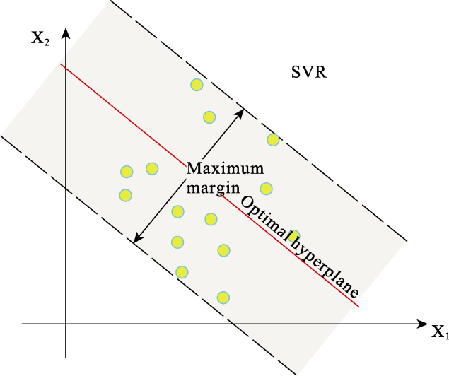
Figure 4 Schematic diagram of the SVR
Suppose training data
( x 11 ,   x 12 , . . . , x 1 n , y 1 ) , . . . ,   ( x l 1 ,   x l 2 , . . . , x ln , y l ) X × R
, where xi1, xi2, …, xln represent the predictor variables and yi represents observed variables. The goal of SVR is to find a function f(x) that makes errors between predictor variables and observed variables less. Mathematically,
f ( x ) = w , x + b , w , x X , b R
where $\langle w,x \rangle$ denotes the dot product in X. w can be obtained by minimizing the Euclidean norm, i.e., $\Arrowvert w \Arrowvert^{2}$. Thus the SVR problem can be formulated as:
min 1 2 w 2 + C i = 1 n ξ i + ξ i *
s . t . y i - f ( x i ) ε + ξ i f ( x i ) - y i ε + ξ i * ξ i , ξ i * 0
where ζi and ζi* are two positive slack variables denoting the training error of the sample with an error tolerance ε. C is a parameter for controlling the model’s empirical risk. To solve this convex quadratic programming problem, the Lagrange function is introduced according to the Karush-Kuhn-Tucker (KKT) condition:
L w , b , a , a * = 1 2 w 2 + C i = 1 n ξ i + ξ i * - i = 1 n a i ξ i + ε - y i + w , ϕ ( x ) + b - i = 1 n a i * ξ i * + ε - y i - w , ϕ ( x ) - b - i = 1 n η i ( ξ i + ξ i * )
The Lagrange dual problem of the original programming problem is obtained:
min 1 2 i , j = 1 n a * i + a i a * j + a j K x i , x j - i = 1 n a i * ( y i - ε ) + i = 1 n a i ( y i - ε ) s . t . i = 1 n a i * - a i = 0 0 a i * , a i C
We solve the dual problem and obtain the optimal solution:
a ¯ = ( a 1 ¯ , a 1 ¯ , . . . , a ¯ n , a n ¯ ) T .
The input of the sample point corresponding to the non-zero vector
a i ¯
or
a i * ¯
in the optimal solution is the support vector. Thus, a nonlinear regression function is constructed as follows:
f x = ( a i ¯ - a i * ¯ ) K x i , x j + b
where
K x i , x j
is the kernel function, and the kernel function used in this paper is the linear function.

2.3.5 Evaluation of the simulation accuracy of the empirical equations

We employ several widely used indexes to evaluate the accuracy, including the coefficient of determination (R2), relative error (RE), and Nash Sutcliffe coefficients (NSE) (Nash and Sutcliffe, 1970) as shown in Eqs.(18)-(20).
R 2 = i = 1 n R s i m , i - R s i m ¯ R o b s , i - R o b s ¯ 2 i = 1 n R s i m , i - R s i m ¯ 2 i = 1 n R o b s , i - R o b s ¯ 2
R E = R m o d , i - R o b s , i / R o b s , i × 100 %
N S E = 1 - i = 1 n ( R o b s , i - R m o d , i ) 2 i = 1 n ( R o b s , i - R o b s , i ¯ ) 2

3 Results

3.1 Investigating critical influencing factors of snowmelt runoff

This section shows the identification of the critical influencing factors using a global sensitivity analysis method. Before identifying the critical factors, the sensitivity of each factor to snowmelt runoff with lags of 0-5 days, is analyzed. As shown in Figure 5a, the sensitivity of solar radiation with a 0 day lag, denoted as R(0), is the largest (0.255) among R(0)-R(5), indicating that the time lag effect of solar radiation on daily snowmelt runoff is 0 days. Similarly, precipitation (P) and relative humidity (RH) show similar behavior, i.e., no time lag effect on daily snowmelt runoff. Temperature (T) and wind speed (W) are found to have a 2-day lag. Compared with the time lag effect of moisture conditions (precipitation and relative humidity), the time lag effect of thermal conditions (temperature and solar radiation) and air flow conditions (wind speed) is more significant. A plausible reason is that moisture conditions affect the snowmelt runoff mainly through the snowmelt process. The thermal and air flow conditions affect the snowmelt runoff through both the snowmelt process and snow sublimation. Among the thermal influence factors, the time lag of solar radiation is more significant than temperature because the ground temperature rise is primarily caused by absorbing solar radiation (Prescott and Collins, 1951).
Figure 5 The sensitivity of each factor to snowmelt runoff with lags of 0-5 days (a-e) and the sensitivity of all factors to snowmelt runoff (f)
Therefore, solar radiation, precipitation, relative humidity on the same day (R(0), P(0), RH(0)), temperature, and wind speed at two days before (T(2), W(2)) are selected as the critical influencing factors. The results show snowmelt runoff is mostly sensitive to solar radiation, followed by air temperature (Figure 5f). It is likely because solar radiation is the primary energy source for snow melting and part of the energy input is used to heat the snow, and the other part is to melt the snow (Meriö, 2015).

3.2 Correlation analysis between snowmelt runoff and influencing factors

The correlations between the snowmelt runoff and influencing factors were analyzed using the geostatistical analysis method described previously. As shown in Figure 6, the relationship between the percentage change of the snowmelt runoff and the change of the meteorological factors is asymmetric where the snowmelt runoff shows a nonlinear response to the meteorological factors. The snowmelt runoff is positively correlated with precipitation and relative humidity but negatively correlated with temperature, solar radiation, and wind. The impact of solar radiation and temperature on snowmelt runoff is closely related to the change in cumulative snowfall. For example, when the total solar radiation increases, the solar radiation is negatively correlated with snowmelt runoff; however, when the solar radiation decreases, the solar radiation impact is positive if the cumulative snowfall changes less. It is because temperature and radiation can affect snowmelt runoff through both the snow melting and sublimation process. When the variation in cumulative snowfall is insignificant, and the solar radiation value is below the multi-year average solar radiation, the solar radiation mainly affects the snowmelt runoff through affecting the snowmelt rate. As the radiation decreases, so does snowmelt runoff. In contrast, when the cumulative snowfall amplitude is large and the radiation decreases, it indirectly affects the snowmelt runoff through sublimation.
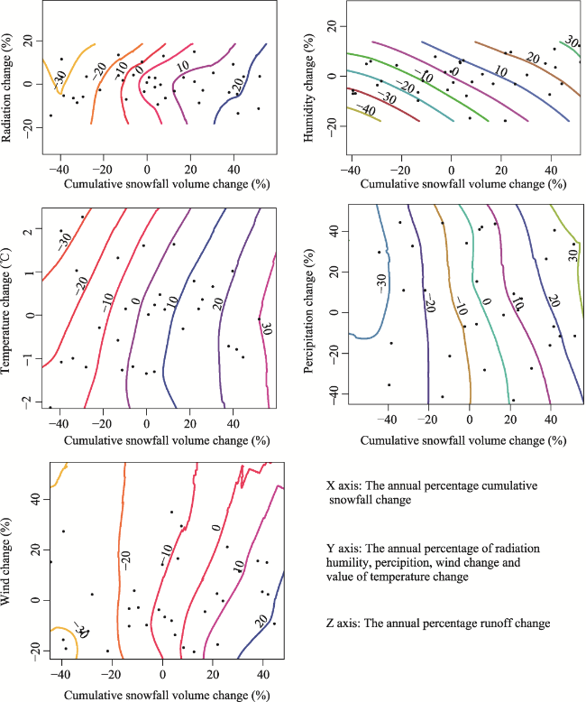
Figure 6 Contour plot of percentage annual snowmelt runoff change as a function of annual percentage solar radiation, precipitation, humidity, wind speed, cumulative snowfall change, and temperature change

3.3 Contribution rate of critical influencing factors to snowmelt runoff

3.3.1 Simulation results

Simulation results from the two empirical models are shown in Figure 7. The coefficient of determination (R2), relative error (RE), and Nash-Sutcliffe efficiency coefficient (NSE) are selected to evaluate the model accuracy. The simulation accuracy of the two empirical models is shown in Table 1, which meets the accuracy requirements as suggested by many researchers (R2 > 0.5 and NSE > 0.4) (Nafees Ahmad et al., 2011), indicating that the models can simulate snowmelt runoff well.
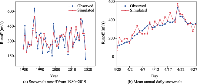
Figure 7 Simulation results of empirical equations on the yearly scale (a) and daily scale (b)
Table 1 Empirical equation simulation results in accuracy
Time scale Calibration (1980-1999) Validation (2000-2019)
R2 NSE RE% R2 NSE RE%
Year 0.83 0.51 16.77 0.65 0.45 16.95
Day 0.67 0.61 17.17 0.63 0.54 9.36

3.3.2 Contribution rate

As shown in Figure 8a, the contribution of temperature and solar radiation to snowmelt runoff, as indicated by the yearly model, is around 56% and 44%, respectively. The higher solar radiation contributions occurred in 2006, 2007, 2010, and 2013 from 1980-2019. It is found that solar radiation made the most significant contribution to snowmelt runoff in 2013 when it was relatively colder, with the lowest average temperature of 0.79℃, below 84% of the annual average, while the solar radiation was close to the annual average. It is worth noting that the average relative humidity was 65% in 2013, and the precipitation was 51mm. It indicates that when the temperature is shallow and the relative humidity is high, the contribution of solar radiation to snowmelt runoff is significant. Also in this case, most energy from solar radiation is used to melt the snow, and only a small part is used to raise the temperature. In comparison, the contribution rate of temperature in 1998 was the highest as the temperature was also the highest from 1980 to 2019, reaching 9℃. Moreover, solar radiation was close to the highest value over the years, reaching 18.9 MJ/m2. In this case, however, most energy from solar radiation is used to raise the temperature, and a small part is used to melt the snow.
Figure 8 Contributions of temperature and solar radiation to snowmelt runoff at yearly (a) and daily (b) scale
As for the daily scale, the contribution rate of solar radiation and temperature to snowmelt runoff is 62% and 38%, respectively (Figure 8b). The difference between daily temperature and solar radiation contribution rate is minor. This is mainly because the variation of the multi-year averaged solar radiation and temperature is small across the month, i.e., from 28 March to 28 April.
Cumulative snowfall and precipitation are important water sources of snowmelt runoff. The contribution rates of cumulative snowfall and precipitation to snowmelt runoff at the yearly scale are 86.43% and 13.57%, respectively (Figure 9). Daily contribution rates of accumulated snowfall and precipitation to snowmelt runoff are 97.68% and 2.32%, respectively. Clearly, the precipitation contribution rate is less than cumulative precipitation because on the one hand, cumulative snowfall is still the primary source of moisture for snowmelt runoff. The cumulative snowfall is the snowfall from 1 November to 27 March in the next year. Precipitation only contains rainfall and snowfall from 27 March to 28 April, which is rare. On the other hand, precipitation mainly affects snowmelt runoff by increasing the ablation rate of accumulated snowfall through enhancing the metamorphism of snow cover (Conway and Benedict, 1994), and improving thermal conductivity (Ocampo Melgar and Meza, 2020).
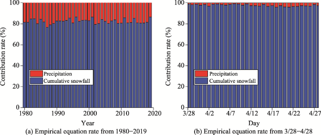
Figure 9 Contributions of cumulative snowfall and precipitation to snowmelt runoff at yearly period (a) and daily scale (b)

3.4 Mid-long term snowmelt runoff forecasting

Following this, two snowmelt runoff forecasting models which have a lead time of one month are developed using the BP neural networks and SVR respectively and the inputs are accumulated snowfall, average solar radiation, and average sunspots during the snowmelt runoff period. This is justified by the fact that accumulated snow is the primary water source of snowmelt runoff in the study area, and solar radiation is one of the critical influencing factors of snowmelt runoff. In addition, sunspots have an essential impact on solar radiation and can be predicted. The forecasting model is trained with the snowmelt runoff data over 1980-2009 and the inputs used are the calculated solar radiation (Duffie and Beckman 1980; Neitsch et al., 2011), the number of sunspots (Li et al., 2019) and the accumulated snowfall from 2010 to 2019.
The accuracy of the forecasting models is assessed against the Chinese national standard, i.e., the Standard for Hydrological Information and Hydrological Forecasting (GB/T 22482-2008, Table 2). According to the standard, ten percent of the multi-year variation of the predictand is taken as the allowable error for the quantitative flow forecast. In our case, the permissible error for the Baishan basin is 49.9 m3·s-1. During the 30 years of the training period, the forecasting model based on BP neural networks (Figure 10a) achieved a qualified rate (QR) of 66.7% (20/30×100%), whilst the qualified rate of the model based on SVR in this period is 70%. For the forecasting period (10 years), the model based on BP neural networks had 6 years of qualified simulations (Figure 10b), hence, the pass rate is 60% (6/10×100%), which achieves a C grade according to Table 2. In comparison, the SVR based model had a QR of 70% and a grade of B. This shows that the SVR method may be more suitable for mid-long term snowmelt runoff prediction in Baishan Basin.
Table 2 Forecast accuracy grade
Grade A B C
Qualified rate (QR) QR≥85% 85%>QR≥70% 70%>QR≥60%
Figure 10 Forecasted snowmelt runoff using BP (a) and SVR (b) and its absolute error (Ae)
To further reveal why the SVR method is superior to the BP neural networks, RMSE indicators (root mean square error) of SVR and BP neural networks are compared since RMSE is more sensitive to outliers (Legates and McCabe Jr, 1999). During the forecasting period, the RMSE for the BP method was 79.63, and for the SVR method was 67.45. That is BP neural network having an over-fitting phenomenon, resulting in poor snowmelt runoff forecasting performance. SVR is built on the principle of structural risk minimization and is based on gradient-based training strategies. Therefore, it can solve overfitting and dimensionality problems (Ren et al., 2018; Yan et al., 2019) and provide relatively good prediction results (Niu et al., 2010; Gaur et al., 2021; Jassim et al., 2022).

4 Discussion

4.1 Achievements and innovations

(1) This paper first analyzes the time lag of meteorological influencing factors on snowmelt runoff. Based on these hysteresis results, a global sensitivity analysis method is used to identify the critical influencing factors of snowmelt runoff. It helps to address the issue that many previous studies ignored the time lag effect and interrelationships among meteorological factors and their joint impacts on snowmelt runoff, as global sensitivity analysis can explore the influence of multiple factors on results simultaneously. The results show that solar radiation is the most sensitive meteorological factor, and the snowmelt runoff is more sensitive to the temperature than precipitation, which is agrees with many previous studies in other parts of China (Luo et al., 2017; Jin et al., 2019).
(2) Previous studies have mainly used the Pearson correlation coefficient (Sedgwick, 2012) to reveal the relationship between meteorological influencing factors and snowmelt runoff (Nabi et al., 2011; Zhang et al., 2014), which is suitable for revealing the degree of linear correlation among variables. In contrast, this paper uses a geostatistical analysis method to reveal the nonlinear correlation between meteorological factors and snowmelt runoff. It was found that the snowmelt runoff is negatively correlated with temperature, solar radiation, and wind speed. This conclusion is consistent with the findings reported by Zhu et al. (2015).
(3) Compared with previous studies (Yang, 2015; Tian et al., 2018), this study significantly has reduced the requirements of multiple input variables for predicting snowmelt runoff, by selecting the critical influencing factors. Based on this, a mid-long term forecasting model with a lead time of one month is implemented. The forecasting model is shown to be able to produce more accurate results compared with those from other methods.

4.2 Applicability and uncertainty

This study shows that using SVR with the selected critical factors is suitable for snowmelt runoff forecasting in cold regions, especially in mountainous areas with insufficient observed data and complex snowmelt runoff processes. To further explore the reliability of the results of SVR, this study analyzed the uncertainty of prediction results with a 90% confidence interval using the hydrological uncertainty processor (HUP) of the Bayesian forecasting system based on the coverage index (CR) (Xiong et al., 2009). The Bayesian Forecasting System is a method proposed by Krzysztofwicz in 1999 to solve the uncertainty problem in hydrological forecasting (Krzysztofowicz, 1999; Krzysztofowicz, 2002). The closer the CR value is to the specified confidence level, the more reliable the results. The CR of SVR forecasting results from 1980-2019 is 88% (Figure 11), close to a 90% confidence interval.
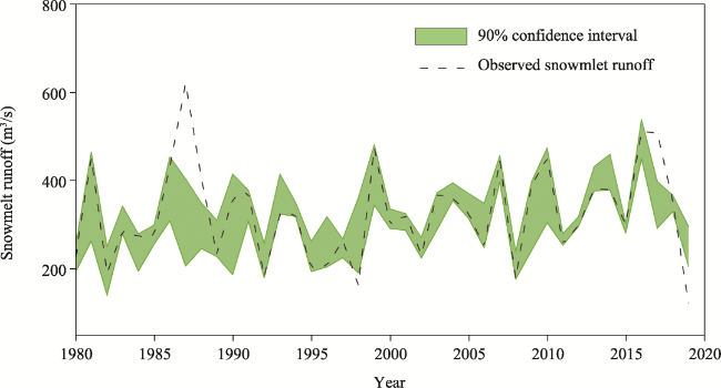
Figure 11 SVR uncertainty analysis results

4.3 Limitations

Although the mid-long term snowmelt runoff forecasting was achieved with fewer data quantities using the BP neural network and SVR model, snowmelt runoff prediction results most likely tend to adapt to major trends rather than extremes. It may lead to an underestimation of the snowmelt runoff peak. Coupling different models is the trend in solving this problem in hydrological research (Hagg et al., 2013; He et al., 2018; Ren et al., 2018). To improve the prediction ability of SVR and BP neural network methods for mid-long term snowmelt runoff, further work is expected to integrate multiple methods with original machine learning methods in future research. For example, the wavelet decomposition pretreatment technology can successfully overcome the non-stationarity of the flow, and the resulting decomposition part of the original sequence represents the specific temporal characteristics of the original series. Integration of wavelet decomposition technique with machine learning methods is expected to improve snowmelt runoff simulation performance.

5 Conclusions

Snowmelt runoff is essential for the integrated management and scheduling of water resources. Due to many meteorological influencing factors and complex physical processes of snowmelt runoff, middle to long term forecasting of snowmelt runoff accuracy is often very low. In this study, we investigate the critical influencing factor of snowmelt runoff before developing a mid-long term snowmelt runoff forecasting. A global sensitivity analysis is first used to investigate the critical influencing meteorological factors and their time lag. To address the complex relationship between influence factors and snowmelt runoff, geostatistical methods were then employed to reveal the correlations, which supports building a new empirical equation to quantitatively evaluate the impact of the key influencing factors on snowmelt runoff. Finally, a mid-long term snowmelt runoff forecasting is developed using the BP neural networks and the SVR. The main findings can be summarized as follows:
(1) Solar radiation is the most critical meteorologic factor of snowmelt runoff, followed by the air temperature. Both factors have different time lags in relation to their influences on snowmelt runoff. The influence of temperature on snowmelt runoff has a 2-day lag, but there is no lag effect of solar radiation.
(2) Snowmelt runoff is negatively correlated with temperature, solar radiation, and wind speed but positively correlated with precipitation and relative humidity. The impact of solar radiation and temperature on snowmelt runoff is closely related to the change in cumulative snowfall.
(3) The contribution rates of solar radiation and temperature at the annual scale to snowmelt runoff are 56% and 44%, respectively. Therefore, solar radiation can be regarded as the critical forecast factor for the mid-long term snowmelt runoff forecast.
(4) The SVR method performs better than BP neural networks in mid-long term snowmelt runoff forecasting.
[1]
Adnan M, Nabi G, Saleem Poomee M et al., 2017. Snowmelt runoff prediction under changing climate in the Himalayan cryosphere: A case of Gilgit River Basin. Geoscience Frontiers, 8(5): 941-949.

DOI

[2]
Barnett T P, Adam J C, Lettenmaier D P, 2005. Potential impacts of a warming climate on water availability in snow-dominated regions. Nature, 438(7066): 303-309.

DOI

[3]
Bergström S, Lindström G, 2015. Interpretation of runoff processes in hydrological modelling: Experience from the HBV approach. Hydrological Processes, 29(16): 3535-3545.

DOI

[4]
Bookhagen B, Burbank D W, 2010. Toward a complete Himalayan hydrological budget: Spatiotemporal distribution of snowmelt and rainfall and their impact on river discharge. Journal of Geophysical Research: Earth Surface, 115(F3).

[5]
Callegari M, Mazzoli P, De Gregorio L et al., 2015. Seasonal river discharge forecasting using support vector regression: A case study in the Italian Alps. Water, 7(5): 2494-2515.

DOI

[6]
Che T, Li X, Jin R et al., 2008. Snow depth derived from passive microwave remote-sensing data in China. Annals of Glaciology, 49: 145-154.

DOI

[7]
Chen G, Wang X, Zhuang Z et al., 1996. Genetic Algorithm and Its Application. Beijing: People Post and Communication Publisher of China.

[8]
Cidan Y, Li H, Yang W et al., 2021. Method to identify composition and production phases of spring runoff in high-latitude mid-temperate regions: A case study in the Second Songhua River Basin, China. Journal of Water and Climate Change, 12(8): 3786-3800.

DOI

[9]
Conway H, Benedict R, 1994. Infiltration of water into snow. Water Resources Research, 30(3): 641-649.

DOI

[10]
Corzo G, Solomatine D, 2007. Knowledge-based modularization and global optimization of artificial neural network models in hydrological forecasting. Neural Networks, 20(4): 528-536.

PMID

[11]
Costa D, Shook K, Spence C et al., 2020. Predicting variable contributing areas, hydrological connectivity, and solute transport pathways for a Canadian Prairie Basin. Water Resources Research, 56(12): e2020W- e27984W.

[12]
Dai L, Che T, Ding Y, 2015. Inter-calibrating SMMR, SSM/I and SSMI/S data to improve the consistency of snow-depth products in China. Remote Sensing, 7(6): 7212-7230.

DOI

[13]
Dewalle D R, Rango A, 2008. Principles of Snow Hydrology. Cambridge: Cambridge University Press.

[14]
Dibike Y B, Velickov S, Solomatine D et al., 2001. Model induction with support vector machines: Introduction and applications. Journal of Computing in Civil Engineering, 15(3): 208-216.

DOI

[15]
Duffie J A, Beckman W A, 1980. Solar Engineering of Thermal Processes. New York: Wiley.

[16]
Feng Z, Niu W, Tang Z et al., 2020. Monthly runoff time series prediction by variational mode decomposition and support vector machine based on quantum-behaved particle swarm optimization. Journal of Hydrology, 583: 124627.

DOI

[17]
Gaur S, Johannet A, Graillot D et al., 2021. Modeling of groundwater level using artificial neural network algorithm and WA-SVR model. In: Groundwater Resources Development and Planning in the Semi-arid Region. Springer: 129-150.

[18]
Guo J, Zhou J, Qin H et al., 2011. Monthly streamflow forecasting based on improved support vector machine model. Expert Systems with Applications, 38(10): 13073-13081.

DOI

[19]
Hagg W, Hoelzle M, Wagner S et al., 2013. Glacier and runoff changes in the Rukhk catchment, upper Amu-Darya Basin until 2050. Global and Planetary Change, 110: 62-73.

DOI

[20]
Hasson S U, Saeed F, Böhner J et al., 2019. Water availability in Pakistan from Hindukush-Karakoram-Himalayan watersheds at 1.5℃ and 2℃ Paris Agreement targets. Advances in Water Resources, 131: 103365.

DOI

[21]
He Y, Pu T, Li Z et al., 2010. Climate change and its effect on annual runoff in Lijiang Basin-Mt. Yulong Region, China. Journal of Earth Science, 21(2): 137-147.

[22]
He Z, Vorogushyn S, Unger-Shayesteh K et al., 2018. The value of hydrograph partitioning curves for calibrating hydrological models in glacierized basins. Water Resources Research, 54(3): 2336-2361.

DOI

[23]
Hock R, Rees G, Williams M W et al., 2010. Contribution from glaciers and snow cover to runoff from mountains in different climates. Hydrological Processes, 20(10): 2089-2090.

DOI

[24]
Jassim M S, Coskuner G, Zontul M, 2022. Comparative performance analysis of support vector regression and artificial neural network for prediction of municipal solid waste generation. Waste Management & Research, 40(2): 195-204.

[25]
Jenicek M, Ledvinka O, 2020. Importance of snowmelt contribution to seasonal runoff and summer low flows in Czechia. Hydrology and Earth System Sciences, 24(7): 3475-3491.

DOI

[26]
Jin H, Ju Q, Yu Z et al., 2019. Simulation of snowmelt runoff and sensitivity analysis in the Nyang River Basin, southeastern Qinghai-Tibetan Plateau, China. Natural Hazards, 99(2): 931-950.

DOI

[27]
Krzysztofowicz R, 1999. Bayesian theory of probabilistic forecasting via deterministic hydrologic model. Water Resources Research, 35(9): 2739-2750.

DOI

[28]
Krzysztofowicz R, 2002. Bayesian system for probabilistic river stage forecasting. Journal of Hydrology, 268(1-4): 16-40.

DOI

[29]
Legates D R, Mccabe Jr G J, 1999. Evaluating the use of “goodness-of-fit” measures in hydrologic and hydroclimatic model validation. Water Resources Research, 35(1): 233-241.

DOI

[30]
Li B, Chen Y, Chen Z et al., 2013. Variations of temperature and precipitation of snowmelt period and its effect on runoff in the mountainous areas of Northwest China. Journal of Geographical Sciences, 23(1): 17-30.

DOI

[31]
Li H, Xie M, Jiang S, 2012. Recognition method for mid- to long-term runoff forecasting factors based on global sensitivity analysis in the Nenjiang River Basin. Hydrological Processes, 26(18): 2827-2837.

DOI

[32]
Li W, Cidan Y, Wang A et al., 2019. Identification of influencing factors and machanism of spring runoff in Baishan watershed, China. Water Resources and Hydropower Engineering, 50(5): 63-72.

[33]
Li W, Li H, Guo X, 2019. Analysis and trend prediction of sunspot activity cycle. Water Resources and Hydropower Engineering, 50(5): 53-62.

[34]
Li Z, Lyu S, Chen H et al., 2021. Changes in climate and snow cover and their synergistic influence on spring runoff in the source region of the Yellow River. Science of The Total Environment, 799: 149503.

DOI

[35]
Li Z, Shi X, Tang Q et al., 2020. Partitioning the contributions of glacier melt and precipitation to the 1971-2010 runoff increases in a headwater basin of the Tarim River. Journal of Hydrology, 583: 124579.

DOI

[36]
Luo K, Tao F, Deng X et al., 2017. Changes in potential evapotranspiration and surface runoff in 1981-2010 and the driving factors in upper Heihe River Basin in Northwest China. Hydrological Processes, 31(1): 90-103.

DOI

[37]
Martinec J, Rango A, Roberts R, 2008. Snowmelt runoff model (SRM) user’s manual. Geographica Bernensia P, 35.

[38]
Meriö L, 2015. The measurement and modeling of snowmelt in sub-Arctic site using low cost temperature loggers. Environmental Engineering: 60-63.

[39]
Montero R A, Schwanenberg D, Krahe P et al., 2016. Moving horizon estimation for assimilating H-SAF remote sensing data into the HBV hydrological model. Advances in Water Resources, 92: 248-257.

DOI

[40]
Nabi G, Latif M, Azhar A H, 2011. The role of environmental parameter (degree day) of snowmelt runoff simulation. Soil & Environment, 30(1).

[41]
Nafees Ahmad H M, Sinclair A, Jamieson R et al., 2011. Modeling sediment and nitrogen export from a rural watershed in eastern Canada using the soil and water assessment tool. Journal of Environmental Quality, 40(4): 1182-1194.

DOI PMID

[42]
Nash J E, Sutcliffe J V, 1970. River flow forecasting through conceptual models (Part I): A discussion of principles. Journal of Hydrology, 10(3): 282-290.

DOI

[43]
Neitsch S L, Arnold J G, Kiniry J R et al., 2011. Soil and water assessment tool theoretical documentation version 2009. Texas Water Resources Institute.

[44]
Niu D, Wang Y, Wu D D, 2010. Power load forecasting using support vector machine and ant colony optimization. Expert Systems with Applications, 37(3): 2531-2539.

DOI

[45]
Ocampo Melgar D, Meza F J, 2020. Exploring the fingerprints of past rain-on-snow events in a central Andean mountain range basin using satellite imagery. Remote Sensing, 12(24): 4173.

DOI

[46]
Ouyang R, Ren L, Cheng W et al., 2010. Similarity search and pattern discovery in hydrological time series data mining. Hydrological Processes, 24(9): 1198-1210.

DOI

[47]
Pomeroy J W, Gray D M, Brown T et al., 2007. The cold regions hydrological model: A platform for basing process representation and model structure on physical evidence. Hydrological Processes, 21(19): 2650-2667.

DOI

[48]
Prescott J A, Collins J A, 1951. The lag of temperature behind solar radiation. Quarterly Journal of the Royal Meteorological Society, 77(331): 121-126.

DOI

[49]
Prestrud P, 2007. Global outlook for ice & snow. UNEP/Earthprint.

[50]
Pyankov S V, Shikhov A N, Kalinin N A et al., 2018. A GIS-based modeling of snow accumulation and melt processes in the Votkinsk Reservoir Basin. Journal of Geographical Sciences, 28(2): 221-237.

DOI

[51]
Qu Y, Li H, Liu H, 2003. Method for optimizing initial weights of ANNS by GAS. Journal of Jilin University Engineering and Technology Edition, 33(2): 11-14.

[52]
Ren G, Cao Y, Wen S et al., 2018. A modified Elman neural network with a new learning rate scheme. Neurocomputing, 286: 11-18.

DOI

[53]
Ren W W, Yang T, Huang C S et al., 2018. Improving monthly streamflow prediction in alpine regions: Integrating HBV model with Bayesian neural network. Stochastic Environmental Research and Risk Assessment, 32(12): 3381-3396.

DOI

[54]
Sciarretta A, Trematerra P, Baumgärtner J, 2001. Geostatistical analysis of Cydia Funebrana (lepidoptera: tortricidae) pheromone trap catches at two spatial scales. American Entomologist, (3): 174-184.

[55]
Sedgwick P, 2012. Pearson’s correlation coefficient. Bmj, 345.

[56]
Siderius C, Biemans H, Wiltshire A et al., 2013. Snowmelt contributions to discharge of the Ganges. Science of the Total Environment, 468: S93-S101.

[57]
Singh P, Ramasastri K S, Kumar N et al., 2000. Correlations between discharge and meteorological parameters and runoff forecasting from a highly glacierized Himalayan Basin. Hydrological Sciences Journal, 45(5): 637-652.

DOI

[58]
Stigter E E, Wanders N, Saloranta T M et al., 2017. Assimilation of snow cover and snow depth into a snow model to estimate snow water equivalent and snowmelt runoff in a Himalayan catchment. The Cryosphere, 11(4): 1647-1664.

DOI

[59]
Tian L, 2019. Research on spring snowmelt runoff in the middle temperate zone: A case study of Baishan Reservoir Basin in the Second Songhua River[D]. Changchun: Jilin University.

[60]
Tian L, Li H, Li F et al., 2018. Identification of key influence factors and an empirical formula for spring snowmelt-runoff: A case study in mid-temperate zone of Northeast China. Scientific Reports, 8(1): 1-12.

[61]
Vapnik V N, 1999. An overview of statistical learning theory. IEEE Transactions on Neural Networks, 10(5): 988-999.

DOI PMID

[62]
Vasil Ev D Y, Gavra N K, Kochetkova E S et al., 2013. Correlation between the total precipitation and the mean and maximum runoff during the snowmelt flood in the Belaya River Basin. Russian Meteorology and Hydrology, 38(5): 351-358.

DOI

[63]
Wang H, Li Y P, Liu Y R et al., 2021. Analyzing streamflow variation in the data-sparse mountainous regions: an integrated CCA-RF-FA framework. Journal of Hydrology, 596: 126056.

DOI

[64]
Wang S, Huang G H, Lin Q G et al., 2014. Comparison of interpolation methods for estimating spatial distribution of precipitation in Ontario, Canada. International Journal of Climatology, 34(14): 3745-3751.

DOI

[65]
Wang S, Huang G H, Veawab A, 2013. A sequential factorial analysis approach to characterize the effects of uncertainties for supporting air quality management. Atmospheric Environment, 67: 304-312.

DOI

[66]
Wang X W, 2010. Study of soil freezing and thawing law and simulation of hydrologic properties in the northern seasonlly frozen soil area[D]. Harbin: Northeast Agricultural University.

[67]
Wheeler D, Shaw G, Barr S, 2013. Statistical Techniques in Geographical Analysis. Routledge.

[68]
Xie S, Du J, Zhou X et al., 2018. A progressive segmented optimization algorithm for calibrating time-variant parameters of the snowmelt runoff model (SRM). Journal of Hydrology, 566: 470-483.

DOI

[69]
Xiong L, Wan M, Wei X et al., 2009. Indices for assessing the prediction bounds of hydrological models and application by generalised likelihood uncertainty estimation. Hydrological Sciences Journal, 54(5): 852-871.

DOI

[70]
Xu Z, Lan Y, Cheng G, 2000. A study on runoff forecast by artificial neural network model. Journal of Glaciology and Geocryology, 22(4): 372-375.

[71]
Yan Z, Liu W, Wen S et al., 2019. Multi-label image classification by feature attention network. IEEE Access, 7: 98005-98013.

DOI

[72]
Yang Q, 2015. Study on spatio-temporal distribution of snow cover in Northeast China and its simulation on snowmelt runoff[D]. Changchun: Jilin University.

[73]
Zhang F, Ahmad S, Zhang H et al., 2016. Simulating low and high streamflow driven by snowmelt in an insufficiently gauged alpine basin. Stochastic Environmental Research and Risk Assessment, 30(1): 59-75.

DOI

[74]
Zhang F, Li L, Ahmad S et al., 2014. Using path analysis to identify the influence of climatic factors on spring peak flow dominated by snowmelt in an alpine watershed. Journal of Mountain Science, 11(4): 990-1000.

DOI

[75]
Zhang Y, Gulimire H, Sulitan D et al., 2022. Monitoring and analysis of snow cover change in an alpine mountainous area in the Tianshan Mountains, China. Journal of Arid Land, 14(9): 962-977.

DOI

[76]
Zhang Z, Kane D L, Hinzman L D, 2000. Development and application of a spatially-distributed arctic hydrological and thermal process model (ARHYTHM). Hydrological Processes, 14(6): 1017-1044.

DOI

[77]
Zhu J, Qi F, Mu X et al., 2015. Snowmelt runoff characteristics and its influencing factors of Songhua River. Bulletin of Soil and Water Conservation, 35(2): 125-130.

Outlines

/