
Journal of Geographical Sciences >
Dynamics of soil loss and sediment export as affected by land use/cover change in Koshi River Basin, Nepal
|
YIGEZ Belayneh, PhD Candidate, E-mail:belayneh@imde.ac.cn |
Received date: 2022-07-19
Accepted date: 2023-03-06
Online published: 2023-06-26
Supported by
Chinese Academy of Sciences (CAS) Overseas Institution Platform Project(131C11KYSB20200033)
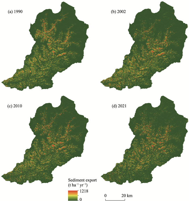
How the dynamics in soil loss (SL) and sedimentation are affected by land use/cover change (LULCC) has long been one of the most important issues in watershed management worldwide, especially in fragile mountainous river basins. This study aimed to investigate the impact of LULCC on SL and sediment export (SE) in eastern regions of the Koshi River basin (KRB), Nepal, from 1990 to 2021. The Random Forest classifier in the Google Earth Engine platform was employed for land use/land cover (LULC) classification, and the Integrated Valuation Ecosystem Services and Trade-offs (InVEST) Sediment Delivery Ratio model was used for SL and SE modeling. The results showed that there was a pronounced increase in forest land (4.12%), grassland (2.35%), and shrubland (3.68%) at the expense of agricultural land (10.32%) in KRB over the last three decades. Thus, the mean SL and SE rates decreased by 48% and 60%, respectively, from 1990 to 2021. The conversion of farmland to vegetated lands has greatly contributed to the decrease in SL and SE rates. Furthermore, the rates of SL and SE showed considerable spatiotemporal variations under different LULC types, topographic factors (slope aspect and gradient), and sub-watersheds. The higher rates of SL and SE in the study area were observed mostly in slope gradient classes between 8° and 35° (accounting for 83%-91%) and sunny and semi-sunny slope aspects (SE, S, E, and SW) (accounting for 57%-65%). Although the general mean rate of SL presented a decreasing trend in the study area, the current mean SL rate (23.33 t ha-1 yr-1) in 2021 is still far beyond the tolerable SL rate of both the global (10 Mg ha-1 yr-1) and the Himalayan region (15 t ha-1 yr-1). Therefore, landscape restoration measures should be integrated with other watershed management strategies and upscaled to hotspot areas to regulate basin sediment flux and secure ecosystem service sustainability.
YIGEZ Belayneh , XIONG Donghong , ZHANG Baojun , BELETE Marye , CHALISE Devraj , CHIDI Chhabi Lal , GUADIE Awoke , WU Yanhong , RAI Dil Kumar . Dynamics of soil loss and sediment export as affected by land use/cover change in Koshi River Basin, Nepal[J]. Journal of Geographical Sciences, 2023 , 33(6) : 1287 -1312 . DOI: 10.1007/s11442-023-2130-x
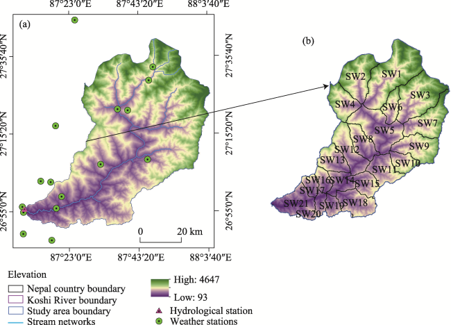
Figure 1 Location of the study area (Koshi River Basin, Nepal): (a) Location and elevation of the study area, and (b) sub-watersheds (SW) of the study. Note: Sub-watersheds in the current study were generated from a 30 m spatial resolution DEM by considering the minimum threshold area of 50 km2 using Arc Hydro tools. |
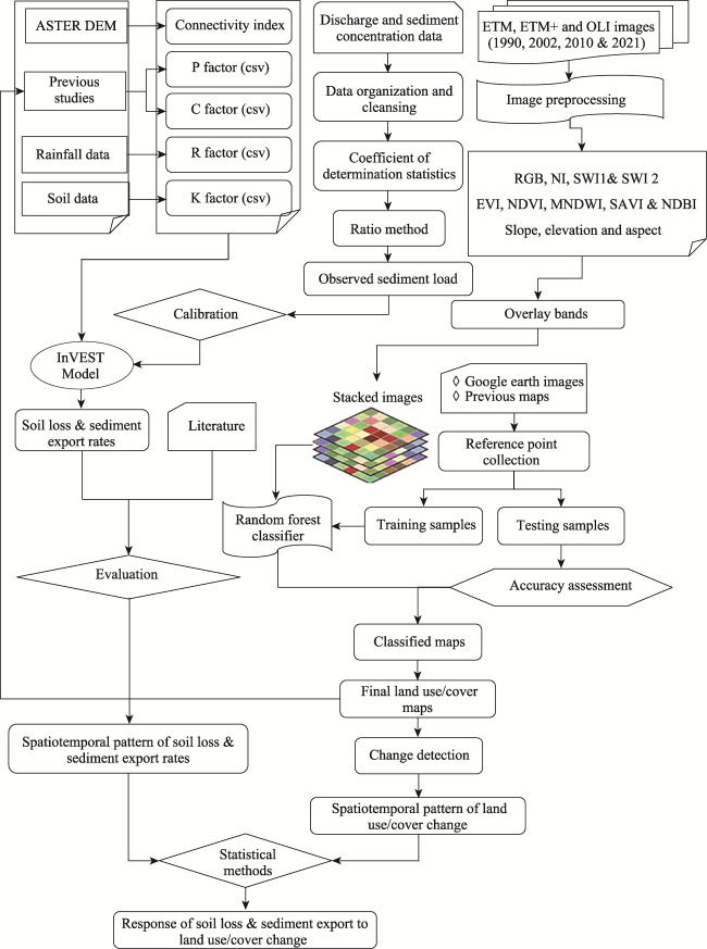
Figure 2 Flow chart of the study methodology |
Table 1 Model performance compared with results of previous studies that have been conducted in the Koshi Basin and Nepal |
| Study area | Methods | SL rate (t ha-1 yr-1) | SE rate (t ha-1 yr-1) | Difference (t ha-1 yr-1) | Author name |
|---|---|---|---|---|---|
| Pakarbas catchment (KRB) | Radionuclide tracing (137Cs and 210Pbex) | 31.29 | -13.92 to 7.96 | Yuan et al. (2021) | |
| Khajuri stream catchment (KRB) | Plot based study | 16 | -29.21 to -7.33 | Ghimire et al. (2013) | |
| Triyuga watershed (KRB) | RUSLE and Williams and Berndt (1972) SDR models | 31 | 3.04 | -14.21-7.67 and -4.45-0.06, respectively | Yigez et al. (2021) |
| The whole Nepal | RUSLE model | 25 | -20.21-1.67 | Koirala et al. (2019) | |
| Kaligandaki River basin (Nepales Himalaya) | SWAT model | 17.3 | 9.81-14.32 | Chinnasamy and Sood (2020) | |
| Jhikhu Khola watershed (KRB) | Radionuclide tracing (137Cs) | 70.17 | 24.96-46.84 | Su et al. (2016) | |
| Current study | InVEST SDR model | 23.33-45.21 | 7.49-2.98 |
Table 2 Soil loss rate, severity classes and priority classes as proposed by Singh et al. (1992) |
| Severity class | Slight | Moderate | High | Very high | Severe | Very severe |
|---|---|---|---|---|---|---|
| SL rate (t ha-1 yr-1) | <5 | 5-10 | 10-20 | 20-40 | 40-80 | >80 |
| Priority class | VI | V | IV | III | II | I |
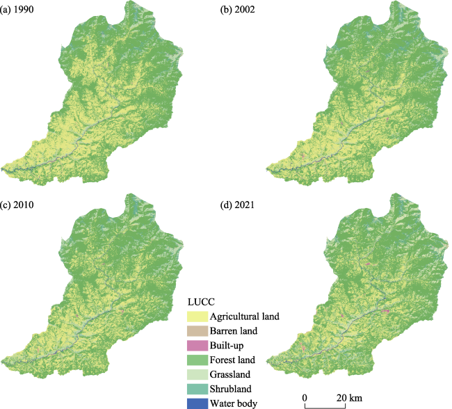
Figure 3 Land use/cover for 1990, 2002, 2010, and 2021 in Koshi River Basin, Nepal |
Table 3 Confusion matrix for classified images |
| LULC | 1990 | 2002 | 2010 | 2021 | ||||||||
|---|---|---|---|---|---|---|---|---|---|---|---|---|
| FS | PA | UA | FS | PA | UA | FS | PA | UA | FS | PA | UA | |
| FT | 90 | 90 | 89 | 90 | 90 | 91 | 94 | 93 | 94 | 95 | 97 | 93 |
| SH | 87 | 79 | 96 | 88 | 85 | 91 | 87 | 83 | 90 | 81 | 75 | 88 |
| GL | 87 | 83 | 90 | 90 | 88 | 92 | 89 | 87 | 91 | 90 | 90 | 90 |
| AG | 91 | 95 | 88 | 91 | 94 | 88 | 92 | 94 | 90 | 95 | 95 | 94 |
| BL | 93 | 88 | 98 | 87 | 87 | 87 | 88 | 87 | 89 | 92 | 94 | 90 |
| WT | 97 | 97 | 98 | 93 | 95 | 90 | 94 | 97 | 92 | 96 | 96 | 96 |
| BU | 90 | 84 | 96 | 84 | 72 | 100 | 91 | 83 | 100 | 97 | 94 | 100 |
| OA | 90 | 90 | 91 | 93 | ||||||||
| KAP | 0.86 | 0.87 | 0.88 | 0.91 | ||||||||
Note: FT-forest land, SH-shrubland, GL-grassland, AG-agricultural land, BL-barren land, BU-built-up area, KAP-Kappa coefficient, OA-overall accuracy, UA-user accuracy, PA-producer accuracy, and FS-F1 score |
Table 4 Areal extent of land use/cover and proportion of land use/cover changes, average soil loss (SL), and sediment export (SE) rate in Koshi River Basin, Nepal from 1990 to 2021 |
| LU class | Area (km2) | Area proportion ∆ (%) | ||||||
|---|---|---|---|---|---|---|---|---|
| 1990 | 2002 | 2010 | 2021 | 1990-2002 | 2002-2010 | 2010-2021 | 1990-2021 | |
| AG | 1176.99 | 973.28 | 892.38 | 744.51 | -4.86 | -1.93 | -5.46 | -10.32 |
| BL | 19.00 | 13.28 | 10.56 | 16.07 | -0.14 | -0.06 | 0.07 | -0.07 |
| BU | 1.00 | 2.31 | 2.51 | 7.54 | 0.03 | 0 | 0.12 | 0.16 |
| FT | 2607.41 | 2702.7 | 2736.2 | 2779.96 | 2.28 | 0.8 | 1.84 | 4.12 |
| GL | 272.65 | 348.35 | 411.49 | 426.61 | 1.81 | 1.51 | 1.87 | 3.68 |
| SH | 100.71 | 136.27 | 124.67 | 199.26 | 0.85 | -0.28 | 1.5 | 2.35 |
| WT | 11.49 | 13.04 | 10.13 | 14.70 | 0.04 | -0.07 | 0.04 | 0.08 |
| SL (t ha-1 yr-1) | 45.21 | 32.18 | 30.31 | 23.33 | -13.03 | -1.87 | -6.98 | -21.88 |
| SE (t ha-1 yr-1) | 7.49 | 4.78 | 4.20 | 2.98 | -2.71 | -0.58 | -1.22 | -4.51 |
Note: FL-forest lands, SH-shrublands, GL-grasslands, AG-agricultural land, BL-barren lands, WT-water, BU- built-up area |
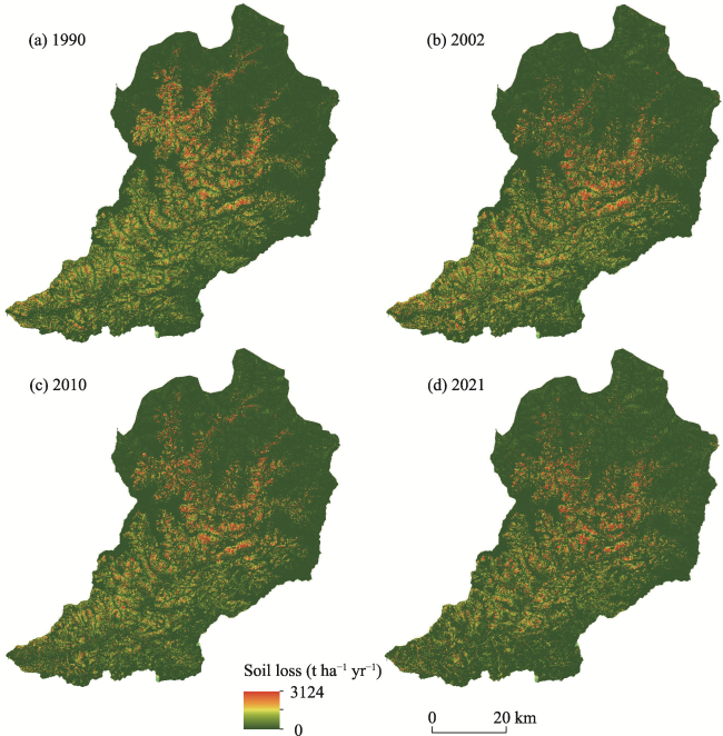
Figure 4 Spatial distribution of soil loss in 1990 (a), 2002 (b), 2010 (c), and 2021 (d) in Koshi River Basin, Nepal |
Figure 5 Spatial distribution of sediment export in 1990 (a), 2002 (b), 2010 (c), and 2021 (d) in Koshi River Basin, Nepal |
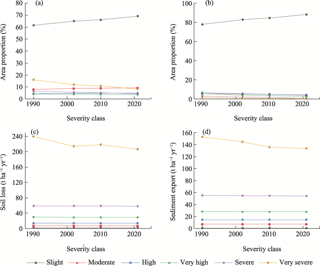
Figure 6 Area proportion of soil loss (a), sediment export (b), and the percentage contribution of each severity class to the basin soil loss (c) and sediment export (d) in 1990, 2002, 2010, and 2021 |
Table 5 Mean (t ha-1 yr-1) and total (*104 t ha-1 yr-1) rate of soil loss and sediment export for different land use/cover from 1990 to 2021 in Koshi River Basin, Nepal |
| Outputs | Year | Forestland | Shrubland | Grassland | Agricultural land | Barren land | Built-up land |
|---|---|---|---|---|---|---|---|
| Mean SL | 1990 | 10.24 | 16.43 | 18.99 | 130.77 | 75.45 | 76.35 |
| 2002 | 7.81 | 11.09 | 18.31 | 107.41 | 78.28 | 10.67 | |
| 2010 | 7.44 | 11.35 | 18.53 | 107.14 | 69.42 | 13.60 | |
| 2021 | 6.36 | 9.74 | 12.92 | 95.20 | 68.81 | 12.36 | |
| Mean SE | 1990 | 1.43 | 2.79 | 2.83 | 22.25 | 16.16 | 17.18 |
| 2002 | 0.98 | 1.66 | 2.36 | 16.52 | 14.91 | 1.36 | |
| 2010 | 0.90 | 1.59 | 2.30 | 15.47 | 13.35 | 1.57 | |
| 2021 | 0.71 | 1.20 | 1.39 | 12.65 | 10.68 | 1.30 | |
| Total SL | 1990 | 267.04 | 16.54 | 51.76 | 1539.10 | 14.33 | 0.76 |
| 2002 | 211.16 | 15.11 | 63.79 | 1045.45 | 10.40 | 0.25 | |
| 2010 | 203.68 | 14.15 | 76.24 | 956.11 | 7.33 | 0.34 | |
| 2021 | 176.80 | 19.41 | 55.10 | 708.79 | 11.06 | 0.93 | |
| Total SE | 1990 | 37.23 | 2.81 | 7.72 | 261.86 | 3.07 | 0.17 |
| 2002 | 26.61 | 2.26 | 8.21 | 160.80 | 1.98 | 0.03 | |
| 2010 | 24.56 | 1.98 | 9.48 | 138.03 | 1.41 | 0.04 | |
| 2021 | 19.81 | 2.39 | 5.94 | 94.17 | 1.72 | 0.10 |
Table 6 Soil loss severity class transition matrix from 1990 to 2021 |
| Year | 2021 | ||||||||
|---|---|---|---|---|---|---|---|---|---|
| Severity class | Slight | Moderate | High | Very high | Severe | Very severe | Total (km2) | (%) | |
| 1990 | Slight | 2378.45 | 48.15 | 30.01 | 21.13 | 36.15 | 74.69 | 2588.57 | 62.00 |
| Moderate | 31.41 | 266.60 | 6.70 | 7.96 | 0.07 | 5.79 | 318.53 | 7.63 | |
| High | 23.63 | 3.64 | 140.11 | 2.72 | 2.16 | 1.45 | 173.71 | 4.16 | |
| Very high | 48.54 | 3.10 | 1.89 | 111.92 | 2.60 | 0.84 | 168.89 | 4.05 | |
| Severe | 120.48 | 0.05 | 0.87 | 2.81 | 133.70 | 4.17 | 262.07 | 6.28 | |
| Very severe | 329.29 | 50.37 | 17.43 | 4.42 | 5.85 | 255.81 | 663.17 | 15.88 | |
| Total (km2) | 2931.79 | 371.92 | 197.02 | 150.95 | 180.53 | 342.74 | 4174.94 | 100.00 | |
| Total (%) | 70.22 | 8.91 | 4.72 | 3.62 | 4.32 | 8.21 | 100.00 | ||
Table 7 Pearson correlation coefficients for the relationship between land use proportion and the average values of soil loss and sediment export in all sub-watersheds from 1990 to 2021 |
| LULC type | 1990 | 2002 | 2010 | 2021 | ||||
|---|---|---|---|---|---|---|---|---|
| SL | SE | SL | SE | SL | SE | SL | SE | |
| FL | -0.45* | -0.51* | -0.39 | -0.47* | -0.55** | -0.57** | -0.21 | -0.32 |
| SH | -0.18 | -0.24 | -0.28 | -0.36 | -0.33 | -0.33 | -0.24 | -0.31 |
| GL | -0.06 | -0.09 | -0.23 | -0.33 | -0.46* | -0.47* | -0.20 | -0.30 |
| AG | 0.64** | 0.63** | 0.69** | 0.77** | 0.68** | 0.70** | 0.71** | 0.75** |
| BL | 0.15 | 0.15 | 0.12 | 0.17 | 0.04 | 0.08 | 0.02 | 0.01 |
| WT | 0.18 | 0.16 | 0.21 | 0.23 | 0.07 | 0.07 | 0.31 | 0.25 |
| BU | -0.08 | -0.05 | 0.29 | 0.18 | -0.08 | -0.07 | 0.36 | 0.36 |
Note: *p<0.05, ** p<0.01; FL-forest lands, SH-shrublands, GL-grasslands, AG-agricultural land, BL-barren lands, WT-water, BU-built-up area |
Table 8 Soil loss and sediment export on different slope gradients in 1990, 2002, 2010, and 2021 in Koshi River Basin, Nepal |
| Slope (°) | Area (km2) | MSL | TSL | ||||||
|---|---|---|---|---|---|---|---|---|---|
| 1990 | 2002 | 2010 | 2021 | 1990 | 2002 | 2010 | 2021 | ||
| 0-5 | 5.94 | 5.78 | 4.72 | 4.82 | 5.10 | 0.34 | 0.27 | 0.23 | 0.25 |
| 5-8 | 9.35 | 16.49 | 13.38 | 13.44 | 13.72 | 1.54 | 2.21 | 1.80 | 1.84 |
| 8-15 | 58.62 | 43.83 | 34.23 | 34.44 | 33.21 | 25.70 | 15.00 | 11.79 | 11.44 |
| 15-25 | 224.57 | 61.13 | 46.39 | 46.30 | 38.37 | 137.29 | 28.36 | 21.48 | 17.77 |
| 25-35 | 249.02 | 43.75 | 30.43 | 26.13 | 18.57 | 108.94 | 13.31 | 7.95 | 4.85 |
| >35 | 177.34 | 30.40 | 17.89 | 16.32 | 8.81 | 53.91 | 5.44 | 2.92 | 1.44 |
| Slope (°) | Area (km2) | MSE | TSE | ||||||
| 1990 | 2002 | 2010 | 2021 | 1990 | 2002 | 2010 | 2021 | ||
| 0-5 | 5.94 | 0.99 | 0.76 | 0.73 | 0.72 | 0.06 | 0.01 | 0.01 | 0.01 |
| 5-8 | 9.35 | 2.79 | 2.08 | 1.99 | 1.89 | 0.26 | 0.06 | 0.04 | 0.04 |
| 8-15 | 58.62 | 7.02 | 4.96 | 4.83 | 4.34 | 4.11 | 0.35 | 0.24 | 0.21 |
| 15-25 | 224.57 | 10.04 | 6.84 | 6.51 | 5.00 | 22.53 | 0.69 | 0.44 | 0.33 |
| 25-35 | 249.02 | 7.40 | 4.63 | 3.64 | 2.36 | 18.41 | 0.34 | 0.17 | 0.09 |
| >35 | 177.34 | 5.01 | 2.61 | 2.10 | 0.97 | 8.88 | 0.13 | 0.05 | 0.02 |
Note: MSL-Mean soil loss (t ha-1 yr-1), TSL-Total soil loss (104 t), MSE-Mean sediment export (t ha-1 yr-1), TSE-Total sediment export (104 t) |
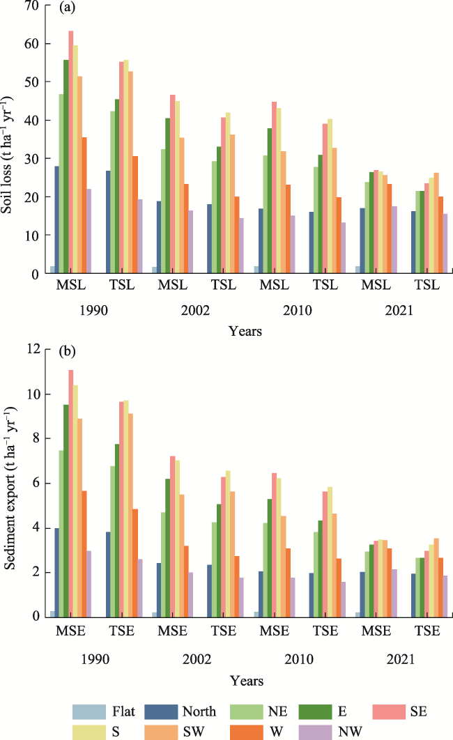
Figure 7 Soil loss in different slope aspects (a) and sediment export in different slope aspects (b) in 1990, 2002, 2010, and 2021 in Koshi River Basin, Nepal(N-north, NE-northeast, E-east, SE-southeast, S-south, SW-southwest, W-west, NW-northwest) |
Table S1 Sources and types of data used in this study |
| Dataset | Source, explanation/purpose |
|---|---|
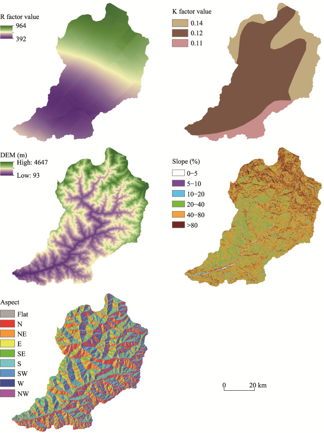
| DEM | We applied a 12.5 m pixel size ASTER GDEM V002 (http://earthexplorer.usgs.gov/) to drive the study area map and topographic factors for the InVEST models. |
| Rainfall data | We used monthly rainfall data of 16 stations from 1989 to 2017 from the Department of Hydrology and Meteorology, Nepal, to calculate the rainfall-runoff erosivity (R) factor of the InVEST model. |
| Soil data | We used a digital soil map (1:5,000,000 scale) consisting of sand, silt, clay, and organic carbon fractions developed by the Food and Agricultural Organization of the United Nations (FAO) and the United Nations Educational, Scientific, and Cultural Organization (UNESCO) (www.fao.org/geonetwork/srv/en/metadata.show?id=14116&currTab=distribution) to calculate the soil erodibility factor of the InVEST models. |
| LULC maps | We used 30 m2 spatial resolution Landsat-5/7/8 images (https://earthengine.google.org) to analyze the spatiotemporal variation of LULC change. |
| SC (g/L) | We used a time series of daily SC data for the years 2006-2013 from the Department of Hydrology Meteorology (DHM), Nepal, to calibrate and validate SL and SE estimation. |
Note: ASTER GDEM V002 = Advanced Space-borne Thermal Emission and Reflection Radiometer Global Digital Elevation Model Version 2; NASA = National Aeronautics and Space Administration; SDR = sediment delivery ratio; InVEST = Integrated Valuation of Ecosystem Services and Tradeoff; LULCC = Land use and land cover; SC = Sediment concentration |
Table S2 InVEST sediment delivery model C and P factor values adopted from previous studies (Wischmeier and Smith, 1978; Kim et al., 2005; Ganasri and Ramesh, 2016; Chalise and Kumar, 2020) |
| LU code | Label | USLE_c | USLE_P |
|---|---|---|---|
| 1 | Forest | 0.003 | 1 |
| 2 | Shrub lands | 0.003 | 1 |
| 3 | Grasslands | 0.01 | 1 |
| 4 | Agricultural lands | 0.63 | 0.5 |
| 5 | Barren lands | 0.45 | 0.7 |
| 6 | Water bodies | 0 | 0 |
| 7 | Snow/Glaciers | 0 | 0 |
| 8 | Built-up | 0.09 | 1 |
Note: USLE_c = cover and management factor; USLE_P = support practice factor |
Table S3 Confusion matrix of land use/cover classification for the year 2021 |
| LULC type | FL | SH | GL | AG | BL | WT | BU | Total | UA (%) | FS |
|---|---|---|---|---|---|---|---|---|---|---|
| FL | 758 | 24 | 8 | 28 | 0 | 0 | 0 | 818 | 93 | 0.95 |
| SH | 10 | 203 | 12 | 3 | 2 | 0 | 0 | 230 | 88 | 0.81 |
| GL | 7 | 18 | 231 | 2 | 0 | 0 | 0 | 258 | 90 | 0.9 |
| AG | 9 | 22 | 6 | 712 | 3 | 0 | 3 | 755 | 94 | 0.95 |
| BL | 0 | 3 | 0 | 2 | 102 | 2 | 4 | 113 | 90 | 0.92 |
| WT | 0 | 0 | 0 | 0 | 2 | 55 | 0 | 57 | 96 | 0.96 |
| BU | 0 | 0 | 0 | 0 | 0 | 0 | 101 | 101 | 100 | 0.97 |
| Total | 784 | 270 | 257 | 747 | 109 | 57 | 108 | 2332 | ||
| PA (%) | 97 | 75 | 90 | 95 | 94 | 96 | 94 | |||
| OA (%) | 93 | |||||||||
| KAP (%) | 91 | |||||||||
Note: FT=forest land, SH=shrubland, GL=grassland, AG=agricultural land, BL=barren land, BU=built-up area, KAP=Kappa coefficient, OA=overall accuracy, UA=user accuracy, PA=producer accuracy, and FS= F1 score |
Table S4 Land use/cover transition matrix from 1990 to 2021 |
| 1990 | 2002 | |||||||
|---|---|---|---|---|---|---|---|---|
| AG | BL | BU | FT | GL | SH | WT | Total | |
| AG | 779.68 | 2.59 | 1.91 | 307.21 | 75.46 | 9.53 | 0.60 | 1176.99 |
| BL | 3.64 | 7.86 | 0.04 | 1.35 | 1.97 | 0.67 | 3.47 | 19.00 |
| BU | 0.52 | 0.05 | 0.25 | 0.17 | 0.01 | 0.00 | 0.00 | 1.00 |
| FT | 144.17 | 1.10 | 0.08 | 2345.82 | 76.36 | 38.53 | 1.36 | 2607.41 |
| GL | 35.78 | 0.52 | 0.02 | 31.57 | 177.97 | 26.72 | 0.07 | 272.65 |
| SH | 8.80 | 0.15 | 0.00 | 15.10 | 15.95 | 60.62 | 0.10 | 100.71 |
| WT | 0.70 | 1.00 | 0.00 | 1.51 | 0.62 | 0.20 | 7.45 | 11.49 |
| Total | 973.28 | 13.28 | 2.31 | 2702.72 | 348.35 | 136.27 | 13.04 | 4189.25 |
| 2002 | 2010 | |||||||
| AG | BL | BU | FT | GL | SH | WT | Total | |
| AG | 691.18 | 1.46 | 1.02 | 185.50 | 68.50 | 24.69 | 0.62 | 972.98 |
| BL | 3.97 | 6.10 | 0.07 | 1.17 | 0.47 | 0.55 | 0.94 | 13.27 |
| BU | 1.02 | 0.00 | 1.04 | 0.22 | 0.02 | 0.00 | 0.00 | 2.31 |
| FT | 145.88 | 0.53 | 0.35 | 2457.62 | 68.05 | 29.29 | 0.47 | 2702.19 |
| GL | 42.62 | 0.69 | 0.02 | 49.76 | 233.88 | 20.88 | 0.16 | 348.01 |
| SH | 6.87 | 0.08 | 0.00 | 39.87 | 40.44 | 48.85 | 0.02 | 136.12 |
| WT | 0.85 | 1.69 | 0.00 | 2.02 | 0.13 | 0.42 | 7.92 | 13.04 |
| Total | 892.38 | 10.56 | 2.51 | 2736.17 | 411.49 | 124.67 | 10.13 | 4187.91 |
| 2010 | 2021 | |||||||
| AG | BL | BU | FT | GL | SH | WT | Total | |
| AG | 557.47 | 3.54 | 4.78 | 211.05 | 78.58 | 36.30 | 0.84 | 892.57 |
| BL | 1.81 | 6.29 | 0.00 | 0.46 | 0.44 | 0.13 | 1.44 | 10.56 |
| BU | 0.62 | 0.05 | 1.67 | 0.15 | 0.02 | 0.00 | 0.01 | 2.52 |
| FT | 150.85 | 1.47 | 0.87 | 2469.99 | 65.77 | 43.68 | 3.85 | 2736.46 |
| GL | 25.75 | 2.63 | 0.21 | 61.87 | 261.68 | 59.39 | 0.18 | 411.70 |
| SH | 7.63 | 0.80 | 0.01 | 36.04 | 20.06 | 59.74 | 0.43 | 124.71 |
| WT | 0.38 | 1.30 | 0.00 | 0.40 | 0.06 | 0.04 | 7.96 | 10.13 |
| Total | 744.51 | 16.07 | 7.54 | 2779.96 | 426.61 | 199.26 | 14.70 | 4188.64 |
Table S5 Dynamics of soil loss (SL), sediment export (SE), and transition in severity class in different sub-watersheds (SWs) of the Koshi River Basin |
| SWs | Area (km2) | SL ( t/ha/year) | SE ( t/ha/year) | ||||||
|---|---|---|---|---|---|---|---|---|---|
| 1990 | 2002 | 2010 | 2021 | 1990 | 2002 | 2010 | 2021 | ||
| SW1 | 534.39 | 34.75 | 19.55 | 14.68 | 13.42 | 5.12 | 2.33 | 1.74 | 1.35 |
| SW2 | 294.23 | 42.63 | 19.22 | 14.92 | 14.28 | 7.17 | 2.23 | 1.71 | 1.48 |
| SW3 | 399.07 | 29.08 | 24.42 | 16.99 | 17.77 | 4.80 | 3.21 | 2.23 | 2.12 |
| SW4 | 189.62 | 53.16 | 25.03 | 21.90 | 20.58 | 8.75 | 3.04 | 2.60 | 2.40 |
| SW5 | 365.17 | 88.66 | 62.13 | 55.03 | 52.72 | 13.76 | 8.67 | 7.57 | 6.66 |
| SW6 | 109.23 | 35.12 | 21.17 | 17.78 | 19.34 | 5.04 | 2.43 | 2.02 | 2.19 |
| SW7 | 264.51 | 18.06 | 16.43 | 12.74 | 13.63 | 2.62 | 2.03 | 1.55 | 1.56 |
| SW8 | 152.88 | 64.60 | 47.68 | 47.03 | 39.03 | 10.59 | 7.11 | 6.78 | 5.38 |
| SW9 | 241.03 | 30.93 | 27.78 | 27.57 | 20.04 | 5.12 | 3.97 | 3.99 | 2.68 |
| SW10 | 110.59 | 27.03 | 22.10 | 26.19 | 19.05 | 3.97 | 2.93 | 3.42 | 2.52 |
| SW11 | 178.08 | 36.53 | 27.82 | 34.25 | 22.46 | 6.06 | 4.15 | 4.98 | 3.26 |
| SW12 | 222.93 | 50.45 | 36.68 | 41.89 | 32.92 | 8.27 | 5.10 | 5.64 | 4.40 |
| SW13 | 161.20 | 59.56 | 41.77 | 48.22 | 32.05 | 10.66 | 6.17 | 6.96 | 4.49 |
| SW14 | 113.44 | 65.07 | 44.77 | 52.05 | 36.08 | 12.69 | 6.94 | 7.80 | 5.19 |
| SW15 | 126.54 | 36.56 | 24.89 | 30.98 | 20.13 | 6.97 | 3.87 | 4.70 | 3.02 |
| SW16 | 78.45 | 64.71 | 47.66 | 52.04 | 35.04 | 11.59 | 6.75 | 7.26 | 4.58 |
| SW17 | 72.45 | 74.87 | 48.44 | 45.53 | 31.51 | 13.63 | 7.00 | 6.35 | 3.91 |
| SW18 | 201.89 | 30.01 | 20.25 | 25.86 | 9.48 | 5.21 | 3.01 | 3.68 | 1.27 |
| SW19 | 65.87 | 38.23 | 24.91 | 27.93 | 13.28 | 7.26 | 4.07 | 4.30 | 2.03 |
| SW20 | 59.36 | 38.51 | 23.34 | 23.45 | 12.45 | 6.90 | 3.31 | 3.16 | 1.60 |
| SW21 | 235.66 | 59.28 | 32.93 | 23.93 | 23.22 | 10.53 | 5.04 | 3.49 | 3.23 |
Table S6 Sediment export severity class transition matrix from 1990 to 2021 |
| Year | 2021 | ||||||||
|---|---|---|---|---|---|---|---|---|---|
| Severity class | Slight | Moderate | High | Very high | Severe | Very severe | Total (km2) | (%) | |
| 1990 | Slight | 3160.71 | 40.32 | 36.20 | 22.96 | 9.94 | 4.10 | 3274.23 | 78.45 |
| Moderate | 127.49 | 84.87 | 4.30 | 0.07 | 0.00 | 0.08 | 216.81 | 5.19 | |
| High | 147.80 | 32.64 | 85.64 | 3.23 | 0.03 | 0.02 | 269.36 | 6.45 | |
| Very high | 132.54 | 0.71 | 29.49 | 54.74 | 1.75 | 0.02 | 219.24 | 5.25 | |
| Severe | 82.19 | 0.01 | 0.61 | 17.23 | 23.84 | 0.65 | 124.52 | 2.98 | |
| Very severe | 51.69 | 0.88 | 0.23 | 0.39 | 6.26 | 10.03 | 69.48 | 1.66 | |
| Total (km2) | 3702.41 | 159.42 | 156.47 | 98.62 | 41.82 | 14.89 | 4173.64 | 100.00 | |
| Total (%) | 88.71 | 3.82 | 3.89 | 2.46 | 1.01 | 0.36 | 100.00 | ||
Figure S1 Spatial distribution of the input data used in this study |
| [1] |
|
| [2] |
|
| [3] |
|
| [4] |
|
| [5] |
|
| [6] |
|
| [7] |
|
| [8] |
|
| [9] |
|
| [10] |
|
| [11] |
|
| [12] |
|
| [13] |
|
| [14] |
|
| [15] |
|
| [16] |
|
| [17] |
FAO/UNESCO, 2007. Digital Soil Map of the World (DSMW), (version 3.6). Rome, Italy.
|
| [18] |
|
| [19] |
|
| [20] |
|
| [21] |
|
| [22] |
|
| [23] |
|
| [24] |
|
| [25] |
ICIMOD, 2018. Understanding Sediment Management. Kathmandu, Nepal.
|
| [26] |
|
| [27] |
|
| [28] |
|
| [29] |
|
| [30] |
|
| [31] |
|
| [32] |
|
| [33] |
|
| [34] |
|
| [35] |
|
| [36] |
|
| [37] |
|
| [38] |
|
| [39] |
|
| [40] |
|
| [41] |
|
| [42] |
|
| [43] |
|
| [44] |
|
| [45] |
|
| [46] |
|
| [47] |
|
| [48] |
|
| [49] |
|
| [50] |
|
| [51] |
|
| [52] |
|
| [53] |
|
| [54] |
|
| [55] |
|
| [56] |
|
| [57] |
|
| [58] |
|
| [59] |
|
| [60] |
|
| [61] |
|
| [62] |
|
| [63] |
|
| [64] |
|
| [65] |
|
| [66] |
|
| [67] |
|
| [68] |
|
| [69] |
|
| [70] |
|
| [71] |
|
| [72] |
|
| [73] |
|
/
| 〈 |
|
〉 |