Research Articles

Spatiotemporal evolution and influencing mechanism of ecosystem service value in the Guangdong-Hong Kong-Macao Greater Bay Area

  • LIU Zhitao , 1, 3 ,
  • WANG Shaojian , 2, * ,
  • FANG Chuanglin 1, 3
Expand
  • 1. Institute of Geographic Sciences and Natural Resources Research, CAS, Beijing 100101, China
  • 2. Guangdong Provincial Key Laboratory of Urbanization and Geo-simulation, School of Geographical Sciences and Planning, Sun Yat-sen University, Guangzhou 510275, China
  • 3. School of Resources and Environment, University of Chinese Academy of Sciences, Beijing 100049, China
*Wang Shaojian, PhD and Professor, specialized in urban geography and urban planning. E-mail:

Liu Zhitao, PhD, specialized in urbanization and its ecological and environmental effects. E-mail:

Received date: 2022-11-16

  Accepted date: 2022-12-22

  Online published: 2023-06-26

Supported by

Fundamental Research Funds for the Central Universities(19lgzd09)

Guangdong Special Support Program

Pearl River S&T Nova Program of Guangzhou(201806010187)

Abstract

Ecosystem services are the media and channels through which ecological elements, structures, functions, and products benefit human society. Regulating the utilization intensity and protection methods of society on the ecosystem according to the ecosystem service value (ESV) and its influencing mechanism is of great significance for achieving the sustainable development goals. This paper takes the Guangdong-Hong Kong-Macao Greater Bay Area (GBA) as the research object and describes the spatiotemporal evolution characteristics of ESV in the GBA from 2000 to 2015. Panel quantile regression is also implemented to increase the understanding of the influencing mechanism of ESV. The main results are as follows: (1) From 2000 to 2015, the total ESV declined with a decreasing rate. The areas of decline were mainly distributed in the central part of the GBA and areas along the Pearl River Estuary. (2) Elasticity index, indicating response of ESV to land use change, reached its peak (1.08). The spatial distribution of elasticity index showed that land use changes brought about more intense ESV variations at the junction of cities. (3) In areas with different ESV levels, the influencing factors have different effects. Land use integrity can only promote ecosystem service capabilities in low-ESV areas. The positive effect of temperature on ecosystem service capacity increases with the increase of ESV, which reflects the self-reinforcement of the ecosystem. Moreover, the negative effect of economic density on ecosystem service capacity decreases with the increase of ESV, which reflects the self-protection of the ecosystem. The combination of such self-reinforcement and self-protection will lead to an ESV gap between the high- and low-ESV areas, and induce the “natural Matthew effect.”

Cite this article

LIU Zhitao , WANG Shaojian , FANG Chuanglin . Spatiotemporal evolution and influencing mechanism of ecosystem service value in the Guangdong-Hong Kong-Macao Greater Bay Area[J]. Journal of Geographical Sciences, 2023 , 33(6) : 1226 -1244 . DOI: 10.1007/s11442-023-2127-5

1 Introduction

Ecosystem services are derived from ecosystem structures, functions, or processes that directly or indirectly contribute to human well-being (Costanza et al., 1997; 2014), and are a collective term for the benefits that humans derive from ecosystems (MEA, 2005). In 1992, the United Nations Environment Office issued the State of the World Environment Report 1972-1992, which sounded the alarm of environmental protection to all countries in the world. In 2000, the United Nations listed “ensuring environmental sustainability” as one of the Millennium Development Goals (MDGs), implying that ecological protection gradually became an important development issue for all countries in the world. In 2005, the United Nations released the Millennium Ecosystem Assessment (MEA) report, which clarified the importance of ecosystem service assessment for ecological conservation. Ecosystem services research on human-nature coexistence has gradually become a global academic hotspot. The spatial patterns of ecosystem services and their evolution reflect the external conditions of regional ecosystems, and the influencing factors of ecosystem services and their mode of action explain the internal mechanisms affecting ecosystems. Grasping the external spatiotemporal evolution of ecosystem services and its intrinsic influencing mechanism is important for identifying regional ecosystem service problems, maintaining regional ecological stability, and promoting regional sustainable development (Guan et al., 2018; Huang et al., 2019a; Qu et al., 2019).
Ecosystem service value (ESV) is a quantitative estimate of ecosystem service capacity, and its assessment methods are mainly divided into two categories: monetary and energetic (Li et al., 2019). Among them, the monetary form of ESV is easy to be understood by the public and used by decision-makers; it can effectively assist in spatial planning, ecological control, and ecological restoration (Crossman and Bryan, 2009; Crossman et al., 2011; de Groot et al., 2012), and is the most widely used assessment method. ESV is the basis for depicting the spatial and temporal evolution of ecosystem services, and its accurate accounting is crucial. However, most studies have only used the “Chinese terrestrial ecosystem service equivalence factor table” proposed by Xie et al. (2003, 2008), which assumes that the same land use type has the same ecosystem service equivalence (Liu et al., 2014; Chen et al., 2018; Huang et al., 2019b), ignoring the potential influence of vegetation luxuriance. In contrast, vegetation affects a variety of ecological processes and plays an important role in ecosystem services such as carbon sink and soil and water conservation, and any accounting of ESV that ignores the growth of vegetation will be obviously inaccurate. Therefore, this paper uses the normalized difference vegetation index (NDVI) to reflect the actual condition of regional vegetation, and combines the equivalent factor method to obtain more accurate and realistic ESV accounting results.
If portraying the spatial pattern of regional ecosystem services is to “know the facts,” exploring the mechanism of regional ecosystem service impacts is to “know the reasons,” which is more helpful to grasp the root causes of ecosystem problems and guide regional ecological construction. The factors influencing ecosystem services can be divided into natural factors (biology, climate, soil, topography) and human factors (land use, social economy). In terms of natural factors, both biological traits and biodiversity affect ecosystem service capacity (Engelhardt and Ritchie, 2001; de Bello et al., 2010; Gamfeldt et al., 2013). The influence of climate on ecosystem services exists in a dual pathway of directly regulating hydrothermal conditions (Wang et al., 2016; Braun et al., 2019) and bringing about indirect effects through influencing biological behavior (Prather et al., 2013). Soil, as a background ecological element for biological growth and hosting, its organic carbon accumulation and water circulation (Wang and Liu, 2013; Milne et al., 2015), and other physicochemical properties have a great impact on ecosystem service functions; topography indirectly regulates ecosystem service functions such as soil retention, water supply capacity, and crop production capacity by influencing ecological conditions such as surface temperature, light intensity, and water storage capacity (Munoz et al., 2014; Han and Dong, 2017; Shoko et al., 2019; Zhu et al., 2019). In terms of human factors, changes in land use type, overall land use pattern, and land use intensity affect the level of ecosystem services (Fu and Zhang, 2014). Socioeconomic factors such as economy and population act as indirect influences on ecosystem services by affecting human social activities such as land development and pollution. The influence mechanism of ecosystem services is complex, and the related studies are not sufficiently deep. Most studies have used correlation analysis (Gong et al., 2017; Zhao et al., 2017; Wang et al., 2020), stepwise regression (Chen et al., 2016; Sun et al., 2018), and logistic regression (Qu et al., 2019) to simply identify the role of influencing factors. Although some studies have considered the interaction between the influencing factors and the spatial variation of the effects (Hou et al., 2018; Dai and Wang, 2020), they have not escaped from the underlying cognitive assumption that the relationship between the independent and dependent variables is fixed, ignoring the possibility that the influencing factors have different effects in regions with different levels of ecosystem services. In contrast, quantile regression models, which can obtain corresponding regression coefficients at different quantile points of the dependent variable, are a frontier regression method in the field of statistics (Chen, 2014). This study introduces the above-mentioned method to explore the differences in the effects of ecosystem service influencing factors at different ESV levels, further improving the understanding of ecosystem service influence mechanisms.
Studies on ecosystem services in China can be divided into three scales according to the research object: local area, urban agglomeration, and national. Value assessment at the local-area scale has the largest number of studies (Deng et al., 2019; You et al., 2019), and the content is mostly focused on the spatial and temporal distribution characteristics of regional ESV, with strong specificity and application, and weak regularity and theory. The national-scale value assessment studies—mainly generated in the early stage of the rise of ecosystem service research—have the characteristics of exploring the spatial distribution patterns of ESV, providing cognition of the national ecosystem service status, and supporting the development of national environmental protection undertakings. For example, He et al. (2005) found that the value of terrestrial ecosystem services was largely consistent with the zonal distribution gradient of vegetation. Wang and Lu (2009) pointed out that economic forest ecosystems have convergent spatial distribution characteristics with hydrothermal conditions and biodiversity. The ESV assessment of national forest and grassland ecosystems has promoted the construction and development of a sustainable economic accounting system in China (Xie et al., 2001; Yu et al., 2005). Research at the urban-agglomeration scale has just started in recent years, and the number of studies is relatively small (Liu et al., 2018; Wang et al., 2019). Overall, there is a lack of research on ecosystem services at the national and urban-agglomeration scales, which have high strategic value for guiding harmonious development of humans and nature. As one of the regions with the highest degree of openness, economic dynamism, and fastest urbanization in China, the high-intensity economic development and urban expansion in the GBA have destroyed the elements, structure, and functions of the original ecological environment, posing a great challenge to its ecological civilization construction. At the same time, as the first greater bay area officially approved by China, the GBA has the strategic responsibility of achieving a high level of coordinated ecological and economic development first and playing a pioneering and exemplary role for other regions. Against the background that China attaches great importance to the construction of ecological civilization, strengthening the study of ecosystem services in the GBA is of great strategic value for supporting the long-term regional development of China.
Therefore, this paper takes the GBA as the research object, introduces the ecological indicator NDVI to improve the precision and accuracy of ESV assessment, and then depicts more accurate spatial and temporal evolution characteristics of ecosystem services. At the same time, we adopt the panel quantile regression model for the first time to explore the differences in the effects of ecosystem service influencing factors at different ESV levels, which opens up a new perspective for the study of ecosystem service influencing mechanisms.

2 Data and methods

2.1 Study area

The Guangdong-Hong Kong-Macao Greater Bay Area (21°25'N-24°30'N, 111°12'E- 115°35'E), together with New York Bay Area, San Francisco Bay Area, and Tokyo Bay Area, is one of the world’s four major bay areas—shouldering the important strategic tasks of opening up to the outside world, promoting the development of “one country, two systems,” and supporting the Belt and Road construction. The GBA consists of nine cities, namely Guangzhou, Shenzhen, Foshan, Dongguan, Huizhou, Zhongshan, Zhuhai, Jiangmen, and Zhaoqing; and two special administrative regions, Hong Kong and Macau (Figure 1), with a total area of 56,000 km2. In terms of natural environment, the GBA has a dense network of rivers and abundant water, with a predominantly subtropical and tropical monsoon climate. The topography is high in the northwest and low in the southeast, with mountains concentrated in the north and plains mainly in the central and coastal areas. In terms of social environment, as of 2019, the population of the GBA exceeded 70 million, and the total GDP reached 11.6 trillion yuan. With 5% of the national population and 0.58% of the national land area, the GBA generates more than 12% of the national GDP, making it one of the most economically dynamic regions in China. High-speed urbanization and economic development bring huge challenges to the construction of ecological civilization in the GBA, and how to realize the synergistic development of economy and ecology has become an important issue for the future development of the GBA.
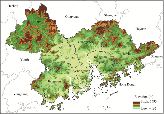
Figure 1 Location of the Guangdong-Hong Kong-Macao Greater Bay Area (GBA)

2.2 Influencing factors and data sources

2.2.1 Influencing factors

The influencing factors of ecosystem services mainly comprise topography, climate, soil, biology, land use type, land use pattern, land use intensity, and socio-economic factors. Due to the limitation of data availability, soil, biological, and land use intensity factors are not included in this paper. Topography factors are not included in this paper because they cannot satisfy the panel data condition due to the availability of 2000 data only. Therefore, the corresponding variables of climate, socio-economic, and land use pattern factors are selected as independent variables in the panel quantile regression. Moreover, although the data form of land use type could not be applied to the panel quantile regression method, land use type is one of the most important influencing factors of ecosystem service (Cord et al., 2017), which can directly affect ESV changes and interactions among ecosystem services (Gomes et al., 2020; Kusi et al., 2020; Schirpke et al., 2020). Considering the importance of the land use type factor and the fact that land use types are susceptible to human regulation, this paper measures the impact of land use type changes on ESV through elasticity coefficients, using global elasticity coefficients to reflect the temporal evolution of land use type impacts on ecosystem service values and local elasticity coefficients to characterize the spatial variation of land use type impacts on ESV.

2.2.2 Regression variables

A total of five independent variables are selected in terms of three influencing factors: climate, socio-economic, and land use structure. In terms of climate, temperature and precipitation are important dimensions characterizing climate conditions and directly influence ESV, with significant spatial variation in their effects (Wang et al., 2016; Braun et al., 2019). Therefore, we select the average annual precipitation (PRE) and the average annual temperature (TEM) as independent variables. In socio-economic aspects, population density indicates the intensity of daily life and economic density indicates the intensity of production activities, and the combination of production and life can reflect the overall socio-economic situation to some extent. Population density (POP) and economic density (GDP) are chosen as independent variables to characterize socio-economics. The data of the above four variables are obtained from the Resource and Environment Science Data Center (RESDC, http://www.resdc.cn). In terms of land use patterns, different land use structures generate different ecological processes and thus provide different levels of ecosystem services (Fu et al., 2013). The average proximity index, which is inversely proportional to the fragmentation of land use structure, reflects the proximity and fragmentation of land use patches and can characterize the land use integrity (Xiao et al., 2001). The mean proximity index (MPI) is selected as the independent variable, and the variable data are obtained using the Patch Analyst module calculated in ArcGIS 10.5. To improve the accuracy of spatial depiction and regression analysis, this paper divides the GBA into a 5 km × 5 km scale grid (2594).
Ecosystem service value (ESV) is used as the dependent variable of this study. Land use data and normalized vegetation index (NDVI) data are applied to account for ESV. Land use data are interpreted from Landsat TM/ETM and Landsat 8 remote sensing images. NDVI data are extracted from SPOT/VEGETATION and MODIS remote sensing images. Both types of data are for four periods—2000, 2005, 2010, and 2015—which are obtained from the RESDC. In this paper, we first reclassify the land use data into six categories: forest, grassland, farmland, construction land, watershed, and unused land. Subsequently, we combine the land classification data, NDVI data, and food price statistics to calculate the ESV of the GBA from 2000 to 2015.

2.3 Methods

2.3.1 Calculation of ESV

Xie et al. (2008) constructed a Chinese ESV equivalent factor table based on the results of Costanza et al. (1997), which is selected as the base equivalent factor table for this paper. Furthermore, by investigating the 2015 Guangdong Statistical Yearbook, China Agricultural Products Price Survey Yearbook, and Guangdong South China Grain Trading Center statistics, the market price of grain per unit production in the GBA is measured, and the base equivalent factor table applicable to the GBA is calculated based on the ESV per unit area of farmland equal to 1/7 of the average grain per unit production market economic value (Table 1). Differences in the degree of vegetation flourishing on land types with vegetation cover (e.g., farmland, woodland, and grassland) can cause the same land types to provide significantly different levels of ecological services (Xu et al., 2012). Therefore, in this paper, the NDVI is used to reflect the vegetation status in the region, and the ESV of the study cells are revised again to finally obtain the ESV of the GBA. The specific formula is:
$SV=\underset{i=1}{\overset{m}{\mathop \sum }}\,\underset{j=1}{\overset{n}{\mathop \sum }}\,\underset{k=1}{\overset{o}{\mathop \sum }}\,{{A}_{ij}}{{B}_{ik}}{{C}_{ik}}$
$~{{C}_{ik}}=\frac{NDV{{I}_{ik}}}{{{\overline{NDVI}}_{i}}}$
where Aij denotes the ecosystem service value coefficient of the jth ecosystem service of the ith land use type, Bik denotes the area of the ith land use type in the kth study cell, Cik denotes the NDVI revision coefficient of the ith land use type in the kth study cell, ${{\overline{NDVI}}_{i}}$ is the mean value of the ith land use type, and NDVIik is the NDVI value of the ith land use type in the kth study cell. i, j, and k denote the land use type, ecosystem service type, and study cell number, respectively, and m, n, and o are the corresponding numbers (m=5, n=9, o=2594).
Table 1 Factor table of ESV per unit area in the GBA (yuan m-2 a-1)
Land use types
Forest Grassland Farmland Watershed Unused land
Providing services 8875 2118 3727 2360 161
Regulating services 38,075 15,820 10,323 97,039 1394
Supporting services 22,872 11,020 6677 10,296 1528
Cultural services 5577 2333 456 11,905 644

2.3.2 Elasticity index

Elasticity is a measure of the degree of response of one variable to changes in another variable. In this paper, we use this approach to measure the percentage change in ESV caused by land use/land cover change (LUCC) (Yuan et al., 2019). The specific formula is:
$E=\left| ~~\frac{(ES{{V}_{{{t}_{1}}}}-ES{{V}_{{{t}_{0}}}})/ES{{V}_{{{t}_{0}}}}}{LUP}~~ \right|~,LUP=\underset{i=1}{\overset{n}{\mathop \sum }}\,\Delta {{L}_{i}}/\underset{i=1}{\overset{n}{\mathop \sum }}\,{{L}_{i}}$
where E denotes the elasticity index of ESV response to land use change, t0 and t1 denote the initial and end period of the study, respectively, LUP denotes the percentage of land use change, ∆Li denotes the area of land use change for the ith land use type, and Li denotes the total area of the ith land use type.

2.3.3 Panel quantile regression model

Panel data have both cross-sectional and temporal dimensions, which increases the sample size relative to cross-sectional or time-series data and can significantly improve the accuracy of regression results. Therefore, this paper analyzes the influencing mechanism of the ESV in the GBA based on four periods of panel data in 2000, 2005, 2010, and 2015. The fixed-effects model and random-effects model are commonly used panel regression models that can identify the relationship between variables as a whole. The Hausman test results show that the fixed-effects model is more suitable for this study, and its specific formula is:
${{y}_{kt}}={{\beta }_{1}}PR{{E}_{kt}}+{{\beta }_{2}}TE{{M}_{kt}}+{{\beta }_{3}}MP{{I}_{kt}}+{{\beta }_{4}}PO{{P}_{kt}}+{{\beta }_{5}}GD{{P}_{kt}}+{{\mu }_{k}}+{{e}_{kt}}$
where β is the regression coefficient,${{y}_{kt}}$is the dependent variable, PREkt etc. are the independent variables, μk is the individual effect whose value is random but does not vary with time, ekt is the disturbance term, and the other parameters are as above.
The panel fixed-effects model focuses on the effect of influence factor x on the conditional expectation E (y | x) of ecosystem service y, but this is actually a mean regression, and in the case where the conditional distribution y | x is not symmetrically distributed, the regression results actually reflect only a part of the relationship between the influencing factor and ecosystem service (Chen, 2014). However, in the quantile regression model, the dependent variable at different quantile points obtains the corresponding coefficient estimates of the independent variables, and it is able to examine the changes in the relationship between influencing factors and ecosystem services in regions with different ESV levels. In addition, quantile regression models based on regression of full sample data can avoid the truncation problem of phased linear regression and have the advantage of being less disturbed by extreme values and can obtain robust coefficient estimates (Koenker and Hallock, 2001). Therefore, in this paper, we use panel quantile regression to explore in depth the factors influencing ecosystem services with the following equation:
${{Q}_{{{y}_{kt}}}}\left( \tau \text{ }\!\!|\!\!\text{ }{{x}_{kt}} \right)={{\beta }_{1}}\left( \tau \right)PR{{E}_{kt}}+{{\beta }_{2}}\left( \tau \right)TE{{M}_{kt}}+{{\beta }_{3}}\left( \tau \right)MP{{I}_{kt}}+{{\beta }_{4}}\left( \tau \right)PO{{P}_{kt}}+{{\beta }_{5}}\left( \tau \right)GD{{P}_{kt}}+{{\mu }_{k}}\left( \tau \right)+{{e}_{kt}}$
where${{Q}_{{{y}_{kt}}}}\left( \tau \text{ }\!\!|\!\!\text{ }{{x}_{kt}} \right)$is the τ conditional quantile of the dependent variable, τ is the quantile (τ ϵ (0, 1)), β(τ) is the regression coefficient at the τ quantile, μk(τ) is the individual effect at the τ quantile, and the other parameters are as above. To show the dynamics of ecosystem service values with the values of influencing factors in more detail, nine quartiles of 0.1–0.9 with 0.1 as the increase were selected as the model quartiles for this study.

3 Results and discussion

3.1 Spatial and temporal evolution of ESV

3.1.1 Temporal evolution of ESV

From 2000 to 2015, the ESV in the GBA continued to decline, from 295.962 billion yuan in 2000 to 282.854 billion yuan in 2015, a total decline of 13.108 billion yuan, with an average annual decline of 874 million yuan. The rapid urbanization in the GBA since the reform and opening up in 1978 has brought enormous pressure on the ecological environment (Luo et al., 2014). Resource consumption and waste emissions from population urbanization have contributed to the reduction of forest biomass and placed pressure on regulating systems such as wetlands. Land use changes induced by spatial, economic, and social urbanization have significantly affected ecosystem service capacity (Zhang et al., 2017), and the ESV in the GBA has declined amid the negative impacts of urbanization. From 2000 to 2005, the ESV declined by 2.36%, accounting for 52.6% of the total decline. However, since 2005, Guangdong Province has implemented the Measures for the Administration of the Transfer of Collective Construction Land Use Rights, which clearly restricts the government’s expropriation of collective construction for real-estate development and can effectively curb market-oriented urban expansion. At the same time, the transfer of collective construction land can prompt rural residents to concentrate in small towns and provide conditions for the re-cultivation of old villages (Tang and Wei, 2006). In 2010, the Guangdong Provincial Government and the State Ministry of Environmental Protection formally signed the Cooperation Agreement on Jointly Promoting and Implementing the Outline of the Plan for the Reform and Development of the Pearl River Delta (2008-2020), and made every effort to promote industrial upgrading and environmental protection infrastructure construction in Guangdong, adopting a series of measures such as no more new coal-fired fuel power plants planned in the Pearl River Delta (PRD) region and banning the construction of highly polluting factories such as ceramic plants and cement plants, which effectively curbed the growth and deterioration of the ecological environment of the PRD region. As a result, the decline of the ESV in the GBA slowed down and stabilized between 2005-2010 and 2010-2015, declining by only 1.05% and 1.08%, respectively. Meanwhile, the four categories of ecosystem sub-services (providing services, regulating services, supporting services, and cultural services) shown in Figure 2 all have similar trends, showing that the ecological conservation measures in the GBA in recent years have begun to bear fruit, and the relationship between humans and nature is gradually improving.
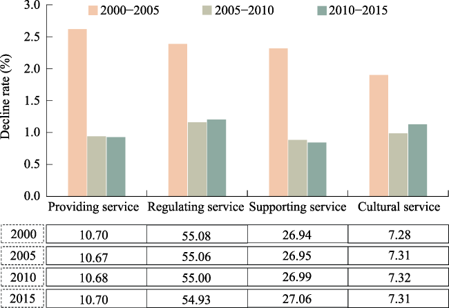
Figure 2 Structure and decline rate of ecosystem sub-service value in the GBA from 2000 to 2015 (%)
In terms of the value structure of ecosystem services in the GBA, the relative proportions of the four types of primary ecosystem services did not change significantly, and the value structure of ecosystem services was relatively stable. Among them, the value of regulating services accounted for the highest proportion, reaching about 55%, which shows that the ecosystem in the GBA mainly plays the role of dissipating human pollution and ensuring ecosystem stability. Accounting for the secondary ecosystem services (food production, raw material production, gas regulation, climate regulation, hydrological regulation, waste treatment, soil conservation, biodiversity, and aesthetic landscape) in the GBA, the results show that the dominant ecosystem service type is hydrological regulating service, and its ESVs from 2000 to 2015 are 552.11, 53.943, 53.199, and 52.481 billion yuan, all taking the top spot in that year, and the decline decreases year by year. The lush vegetation of the GBA and the self-regulating capacity of the Pearl River have provided strong support for hydrological regulating services, and combined with a series of anthropogenic water management measures such as the South Guangdong Clearer Water Action Plan, the water environment in the GBA is expected to further improve. The value of food production services in the GBA is the lowest, with an annual average of less than 7 billion yuan, which is closely related to the industrial characteristics of focusing on the development of manufacturing and service industries.

3.1.2 Spatial distribution of ESV

There are obvious spatial divergences in the changes of ESV in different periods (Figure 3). From 2000 to 2005, 45.77% of the space in the GBA had declining ESV—mainly distributed in the central part of the GBA, both sides of the Pearl River Estuary, central Zhaoqing, and northern Huizhou—which basically overlapped with the space of urban construction land. From 2005 to 2010, the percentage of space where the ESV decreased in the GBA shrank to 42.07%. The space of decline shifted from the central to the periphery of the GBA, distributed in the northwestern part of Zhaoqing, Jiangmen, and most parts of Huizhou. In contrast, the ESV increased in Guangzhou, Dongguan, Shenzhen, Zhuhai, and Zhongshan. The difference in urban development stages is an important reason for this shift. During the 2005-2010 period, most of the space in the central part of the GBA and on both sides of the Pearl River estuary was converted into urban construction land, and cities entered the “stock utilization” stage of construction land, when they focused on improving the efficiency of using existing construction land and reduced the occupation of ecological land. In contrast, the peripheral cities in the GBA are still in the stage of “incremental expansion” of construction land, and the growth rate of urban construction land is relatively fast. In addition, the “double transfer” strategy implemented by Guangdong Province since 2008 has promoted the transfer of labor-intensive industries to the peripheral cities in the GBA, the eastern and western wings of Guangdong, and the mountainous areas in northern Guangdong. The pressure of environmental pollution in the central part of the GBA has also shifted to the periphery in this process. During 2010-2015, the spatial share of reduced ESV in the GBA further shrank to 38.25%, with a fragmented spatial distribution of decline and only small-scale clustering in southern Zhaoqing. As a whole, from 2000 to 2015, the ESV in the GBA decreased over a large area. Among them, the regions with large decreases (more than 1 million yuan) were mainly concentrated in the central part of the GBA and the east coast of the Pearl River Estuary, especially in Dongguan and Shenzhen.
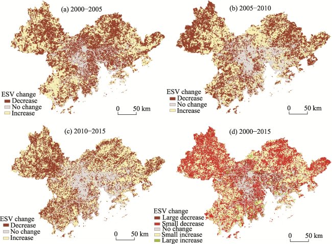
Figure 3 Spatial distribution of ESV variation in the GBA from 2000 to 2015
The hotspot analysis is further used to reveal the spatial clustering characteristics of ESV and its evolution patterns in the GBA from 2000 to 2015 (Figure 4). The spatial clustering characteristics of ESV in half of the GBA are not significant, and the significant areas are dominated by the spatial clustering of high ESV. The high-ESV areas are concentrated in the northeastern and northwestern mountainous areas of the GBA, whereas the low-ESV areas are concentrated in the central part, both sides of the Pearl River estuary, and the coastal area. From 2000 to 2015, the high-ESV area did not change significantly during 2000-2015, whereas the low-ESV area underwent a significant expansion from 2000 to 2005, with the expansion area mainly distributed in Dongguan and Shenzhen. In general, there are obvious zoning differences in ecosystem services within the GBA, with the central and coastal regions becoming the “front line” for urbanization, and the northern mountainous areas becoming the “logistical areas” for ecosystem service.
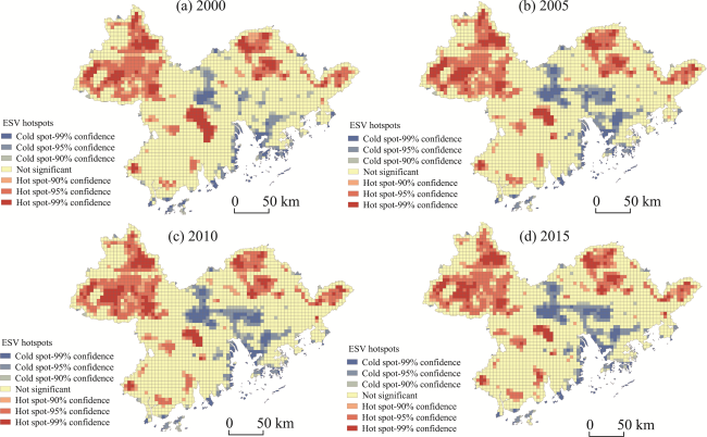
Figure 4 Spatial agglomeration characteristics of ESV in the GBA from 2000 to 2015

3.2 ESV response to land use change

Land use change has a significant impact on ecosystem services (Liu et al., 2015; Li et al., 2016; Guo et al., 2019). In this paper, an elasticity index is introduced to reflect the response of ESV to land use change. During 2000-2015, the area of land use change in the GBA reached 5440.02 km2—mainly concentrated in Dongguan, Guangzhou, Foshan, Zhongshan, Shenzhen, and Zhuhai. Land use types changed the fastest from 2000 to 2005, with a change area of 3585 km2 (Figure 5). The average elasticity of ESV change in the GBA with respect to land use change was 0.38 and 0.31 during 2000-2005 and 2005-2010, respectively, but it jumped to 1.08 during 2010-2015. This result indicates that the disturbance of land use change on ecosystem services was weak during 2000-2010, whereas it increased substantially during 2010-2015. The large area of land use change during 2000-2010 but the lower average elasticity index is due to the fact that the land use conversion in this period was in various directions, including the conversion of forest land and arable land to construction land, and the conversion of forest land and water area to arable land, and the reduction of ESV per unit area of land use change is less. The area of land use change from 2010 to 2015 is small, but it is mainly the conversion of ecological land to urban construction land. This conservation implies the complete loss of ecosystem service capacity and a large change of ESV, which is manifested by a high average elasticity index. From this perspective, the GBA should strengthen the scientific management of urban construction land expansion in the future.
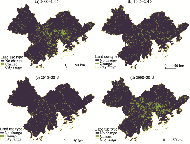
Figure 5 Land use change in the GBA from 2000 to 2015
Precise spatial statistics of the elasticity index during 2000-2015 show that it is higher in the central part of the GBA (Figure 6). The high elasticity index cell clusters at city junctions, and this phenomenon is particularly evident at the Guangzhou-Foshan and Shenzhen-Dongguan junctions. The junctions of Zhaoqing, Huizhou, and Jiangmen with other relatively developed cities also exhibit the characteristics of high elasticity index cell clustering. Since 2009, when the strategic concepts of Guangzhou-Foshan-Zhaoqing, Shenzhen-Dongguan- Huizhou, and Zhuhai-Zhongshan-Jiangmen economic circles were proposed, the level of integration in the GBA has been increasing. Moreover, the construction and human activities at urban junctions have brought about significant declines in ecosystem services. With the increasing connection within the GBA, the urban junction, as the most direct area of urban interaction, is also at risk of ecological land occupation and decline of ecosystem services in the future. How to achieve a win-win situation for ecological protection and economic development through land transfer and innovative land development modes is an important direction to consider for future land use management in the GBA.
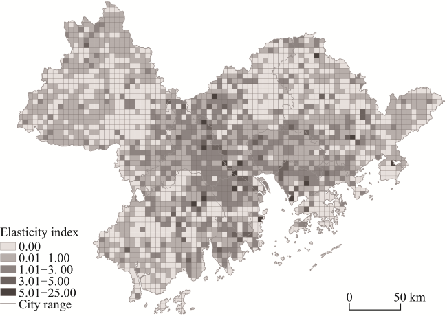
Figure 6 Distribution of elasticity index in the GBA from 2000 to 2015

3.3 Influencing mechanisms of ESV

The panel fixed-effects regression belongs to linear regression, which has a strict assumption of a normal distribution for the dependent variable, whereas the data of the dependent variable in this paper show the distribution characteristics of low kurtosis and left skewness, which rejects the assumption of a normal distribution, so we use the Bloom algorithm to normalize the dependent variable. In contrast, quantile regression does not strongly require that the assumptions of the error term must be satisfied and can be robustly estimated for non-normally distributed variables (Koenker and Hallock, 2001), so the original data are still used in the quantile regression. In addition, the presence of heteroskedasticity reduces the efficiency of panel fixed-effects regressions, and this paper uses robust standard errors to address the heteroskedasticity problem (Chen, 2014). The panel quantile regression is conducted in nine quartiles in this paper, and the specific results are shown in Table 2.
Table 2 Panel regression results of factors influencing ESV in the GBA from 2000 to 2015
Model Coefficients and standard errors
PRE TEM POP GDP MPI
Fixed-effects regression -1.47E-06
(1.59E-06)
1.69E-03***
(5.11E-04)
2.48E-06
(2.58E-06)
-2.92E-06***
(1.11E-06)
1.49E-02
(1.74E-02)
q0.1 regression -121.24
(98.43)
84723.41**
(33532.16)
-431.80
(472.47)
-145.72**
(60.14)
1897395.00**
(859333.60)
q0.2 regression -87.22
(79.58)
87474.14***
(27111.55)
-252.42
(382.00)
-144.63***
(48.63)
1612107.00**
(694778.80)
q0.3 regression -63.99
(68.81)
89352.91***
(23441.90)
-129.90
(330.35)
-143.88***
(42.04)
1417254.00**
(600800.40)
q0.4 regression -40.98
(60.89)
91213.39***
(20740.32)
-8.58
(292.48)
-143.14***
(37.20)
1224297.00**
(531790.40)
q0.5 regression -10.60
(56.55)
93670.10***
(19251.33)
151.63
(271.84)
-142.16***
(34.52)
969503.20**
(494041.20)
q0.6 regression 25.10
(61.81)
96557.23***
(21051.82)
339.91
(297.04)
-141.00***
(37.75)
670069.60
(539974.70)
q0.7 regression 56.87
(74.11)
99126.38***
(25245.84)
507.45
(355.97)
-139.98***
(45.28)
403615.10
(647257.80)
q0.8 regression 91.41
(92.21)
101919.10***
(31414.65)
689.57
(442.78)
-138.87**
(56.34)
113968.60
(805223.40)
q0.9 regression 134.27
(118.18)
105384.80***
(40262.84)
915.57
(567.26)
-137.48*
(72.21)
-245464.60
(1031756.00)

Notes: Robustness standard errors are in parentheses. * indicates p<0.1, ** indicates p<0.05, *** indicates p<0.01.

The panel fixed-effects regression results showed that only TEM and GDP had significant effects on the ESV in the GBA. The positive regression coefficient of TEM indicates that the heat conditions provided by high temperatures contribute significantly to the enhancement of ecosystem quality and ecosystem service capacity. The negative regression coefficient of GDP indicates that human economic activities have a significant coercive effect on the ecological environment, and that high-intensity economic development significantly reduces the ESV.
The results of the panel quantile regression reveal in more detail how the regression coefficients and significance of each variable change with quantile changes, which can help to understand the reasons for the insignificance of some variables in the panel fixed-effects regression and the segmental effects of significant variables. The results of the panel quantile regressions of PRE, POP, and MPI show that the regression coefficients of all three independent variables shift positively and negatively, and this inconsistency in the effects is an important reason for the insignificant results of the panel fixed-effects regressions. The regression coefficient of MPI is significantly positive at the 5% level, implying that the higher the land use integrity, the higher the ESV in areas with low value of ecosystem services. It can be seen that in urban built-up areas where human activities are frequent, ensuring land use integrity and contiguity has a positive effect on increasing ESV.
The panel quantile regression results of TEM show that the regression coefficients of the 0.1 to 0.9 quantiles are significantly positive and gradually increasing, that is, the higher the ESV, the greater the contribution of temperature increase to the improvement of ecosystem service capacity. As a key element of the ecosystem, plants participate in various services such as raw material production, climate regulation, hydrological regulation, and soil conservation, and their growth status plays a decisive role in the ecosystem service function. ESV can also reflect the prosperity of plants. The positive effect of temperature on the enhancement of ecosystem service capacity is therefore more significant in high-ESV areas. The above results suggest that natural conditions such as temperature have a “natural Matthew effect” on ecosystem services. Areas with high ESV have a strong ability to use water and heat to further enhance ecosystem services, whereas areas with low ESV have a weak ability to use water and heat and the rate of ecosystem services enhancement is slow, and the gap between them will be further widened.
The panel quantile regression results of GDP show that the regression coefficients of the 0.1 to 0.9 quantile are all significantly negative and gradually increasing, implying that the higher the value of ecosystem services, the less the economic activities press on ecosystem services. This paper suggests that the reason for this pattern is that the high-ESV areas tend to be pristine and unexplored ecosystems, where few and low-intensity economic activities occur, and the negative impacts of economic activities are weak. The low-ESV areas tend to be more intensely developed areas with higher economic levels, and the negative impacts of economic activities on ecosystem services are significant. It can be seen that although pristine ecological environments far from human society have the strongest ecosystem service capacity and are worthiest of protection, their poor economic development conditions likewise add to their innate protection. In contrast, peri-urban ecosystems close to human society already have a certain basis for economic development and are most vulnerable to coercion from economic activities. In future ecological control in the GBA, emphasis should be placed on protecting partially developed ecosystems from further damage.
The results of the panel quantile regressions give us new insights into the influencing mechanisms of ecosystem services as shown in Figure 7. Self-reinforcement: High-ESV areas with more lush vegetation, richer species, and more efficient ecological cycles are more capable of utilizing natural energy, and their ESV accumulates naturally at a faster rate compared to low-ESV areas. Self-protection: High-ESV areas tend to be spatially located in areas far from cities and will be protected from destruction by constraints such as topography and transportation distance. Low-ESV areas, on the other hand, tend to be located in environments closer to areas of human activity and face greater pressure for anthropogenic development. On the whole, high-ESV areas are significantly stronger than low-ESV areas in terms of self-reinforcement and self-protection capabilities, and the ESV gap between regions will continue to grow in this feedback mechanism.
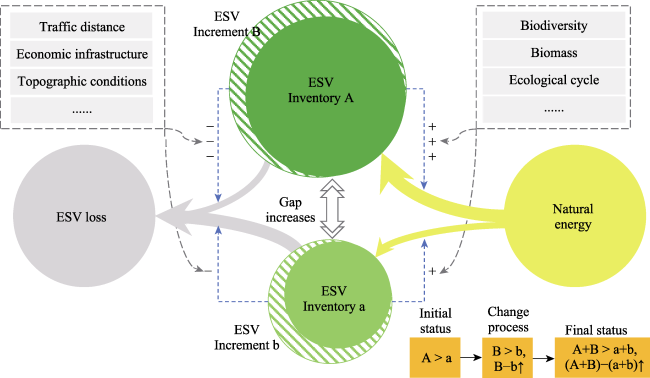
Figure 7 Self-reinforcement and self-protection mechanism of ecosystem service value evolution

4 Conclusions

This paper reveals the spatial and temporal evolution characteristics of the ESV in the GBA, deeply explores the influencing mechanism of the ESV, and obtains the following conclusions:
(1) From 2000 to 2015, the ESV in the GBA continued to decline, totaling 13.108 billion yuan. However, the rate of decline has slowed down significantly since 2005. The values of four sub-services of ecosystem services have a similar trend to the total ESV, among which the value of regulating services has the highest proportion, and hydrological regulating services, which are subordinate to regulating services, are the dominant service type in the GBA. Further analysis of the spatial distribution of ecosystem service value changes revealed that the central part of the GBA and the two sides of the Pearl River estuary are the areas with the greatest decline in ESV. The high-ESV areas are concentrated in the mountainous areas in the northern part of the GBA.
(2) The effect of land use change on the ESV in the GBA was weak in 2000-2010 but strong in 2010-2015. During 2010-2015, the area of land use change in the GBA was small, but the proportion of ecological land converted into urban construction land was higher, bringing about strong changes in ESV. The local elasticity indexes from 2000 to 2015 show that the areas with large ESV impacts from land use change are mainly distributed in urban junctions.
(3) Land use integrity is positively correlated with ESV only in low-ESV areas. The positive effect of temperature on ESV is stronger in areas with higher ESV. The negative effect of economic density on ESV is weaker in areas with higher ESV. Regions with high ESV are highly self-reinforcing and weakly stressed by human activities, whereas the opposite is true for regions with low ESV. Without external intervention, such mechanisms will continue to widen the gap between areas with high and low ESV, creating a “Matthew effect” in ecosystems. Areas with low ESV lack the conditions for natural enhancement and are more vulnerable to human destruction, and should be the focus of ecological protection in the GBA.

5 Limitations and policy implications

As a bridge between the natural environment and human well-being, the study of ecosystem services has become an important issue in the field of human-nature relations research (Zhao et al., 2018). The ESV translates ecological issues into the form of indicators that can be easily interpreted in the public domain to help identify problems, whereas the investigation of ecosystem service influencing mechanisms can help solve problems. Therefore, it must be ensured the ESV assessment reflects the actual situation with good accuracy. As the relationship between humans and nature evolves, the equivalence factor table needs to be updated dynamically to suit the times. With the support of advanced technology, more time-sensitive and local ecological indicators and high-precision remote sensing data should be incorporated into ESV assessment. As a future direction of ESV assessment, models can fully consider ecological processes. In-depth and spatially oriented analysis of ESV influencing mechanisms has high theoretical significance and practical value. Panel quantile regression can divide the dependent variables by quantile points to obtain the impact effects at different ESV levels and then understand the influencing mechanism in depth. However, due to the limitation of model characteristics, non-time-varying factors such as topography cannot be included in the study, and there is the problem of incomplete analysis of the influencing mechanism, which can be combined with other methods to explore the complete influencing mechanism in the future.
Based on the above analysis, the following policy insights are obtained: (i) the ESV at urban junctions is most vulnerable to changes in land use types. With the accelerated integration and networking process in the GBA, strictly controlling the expansion of built-up areas in urban junction areas and improving the intra-city ecological land occupation mechanism are important countermeasures to maintain ecosystem service capacity. (ii) The land use integrity of human gathering areas helps to improve the ESV. For cities in the GBA, continuous expansion of construction land should be the main focus to reduce the ecological land fragmentation caused by urban enclaves, while making full use of the unused land interspersed with construction land. For villages in the GBA, the spatial fragmentation of rural settlements can be appropriately reduced through village integration, which not only saves land resources but also reduces the fragmentation of natural ecosystems by water, electricity, and road networks in rural settlements, and improves the efficiency of social services of administrative and public resources (Long and Tu, 2017). (iii) We should prioritize the protection of ecological environments with low value of ecosystem services, break the “Matthew effect” of ecosystem services by relying on remote sensing technology and accountability systems, and ensure the balanced development of ecosystem service capacity in the whole GBA.
[1]
Braun D, Jong R, Schaepman M E et al., 2019. Ecosystem service change caused by climatological and non-climatological drivers: A Swiss case study. Ecological Applications, 29(4): e01901.

DOI

[2]
Chen D L, Chen Z F, Peng B F, 2018. Spatial differentiation and coupling effect between land ecosystem services value and economic development: A case study of West Dongting Lake area. Geographical Research, 37(9): 1692-1703. (in Chinese)

DOI

[3]
Chen Q, 2014. Advanced Econometrics and Stata Application. Beijing: Adv. Educ. Publishing House.

[4]
Chen S S, Liu K, Bao Y B et al., 2016. Spatial pattern and influencing factors of water conservation service function in Shangluo city. Scientia Geographica Sinica, 36(10): 1546-1554. (in Chinese)

DOI

[5]
Cord A F, Bartkowski B, Beckmann M et al., 2017. Towards systematic analyses of ecosystem service trade-offs and synergies: Main concepts, methods and the road ahead. Ecosystem Services, 28: 264-272.

DOI

[6]
Costanza R, Darge R, De Groot R et al., 1997. The value of the world’s ecosystem services and natural capital. Nature, 6630(387): 253-260.

[7]
Costanza R, De Groot R, Sutton P et al., 2014. Changes in the global value of ecosystem services. Global Environmental Change, 26: 152-158.

DOI

[8]
Crossman N D, Bryan B A, 2009. Identifying cost-effective hotspots for restoring natural capital and enhancing landscape multi-functionality. Ecological Economics, 68: 654-668.

DOI

[9]
Crossman N D, Bryan B A, Summers D M, 2011. Carbon payments and low-cost conservation. Conservation Biology, 25(4): 835-845.

DOI PMID

[10]
Dai E F, Wang Y H, 2020. Spatial heterogeneity and driving mechanisms of water yield service in the Hengduan Mountain region. Acta Geographica Sinica, 75(3): 607-619. (in Chinese)

DOI

[11]
De Bello F, Lavorel S, Diaz S et al., 2010. Towards an assessment of multiple ecosystem processes and services via functional traits. Biodiversity and Conservation, 19(10): 2873-2893.

DOI

[12]
De Groot R, Brander L, Van Der Ploeg S et al., 2012. Global estimates of the value of ecosystems and their services in monetary units. Ecosystem Services, 1(1): 50-61.

DOI

[13]
Deng C X, Zhong X L, Xie B G et al., 2019. Spatial and temporal changes of land ecosystem service value in Dongting Lake area in 1995-2015. Geographical Research, 38(4): 844-855. (in Chinese)

DOI

[14]
Engelhardt K A, Ritchie M E, 2001. Effects of macrophyte species richness on wetland ecosystem functioning and services. Nature, 411(6838): 687-689.

DOI

[15]
Fu B J, Wang S, Su C H et al., 2013. Linking ecosystem processes and ecosystem services. Current Opinion in Environmental Sustainability, 5(1): 4-10.

DOI

[16]
Fu B J, Zhang L W, 2014. Land-use change and ecosystem services: Concepts, methods and progress. Progress in Geography, 33(4): 441-446. (in Chinese)

[17]
Gamfeldt L, Snall T, Bagchi R et al., 2013. Higher levels of multiple ecosystem services are found in forests with more tree species. Nature Communications, 4(1): 1-8.

[18]
Gomes L C, Bianchi F J, Cardoso I M et al., 2020. Land use change drives the spatio-temporal variation of ecosystem services and their interactions along an altitudinal gradient in Brazil. Landscape Ecology, 35(7): 1571-1586.

DOI

[19]
Gong S H, Xiao Y, Zheng H et al., 2017. Spatial patterns of ecosystem water conservation in China and its impact factors analysis. Acta Ecologica Sinica, 37(7): 2455-2462. (in Chinese)

[20]
Guan Q C, Hao J M, Shi X J et al., 2018. Study on the changes of ecological land and ecosystem service value in China. Journal of Natural Resources, 33(2): 195-207. (in Chinese)

[21]
Guo C Y, Gao S, Zhou B Y et al., 2019. Effects of land use change on ecosystem service value in Funiu Mountain based upon a grid square. Acta Ecologica Sinica, 39(10): 3482-3493. (in Chinese)

[22]
Han H Q, Dong Y X, 2017. Assessing and mapping of multiple ecosystem services in Guizhou Province, China. Tropical Ecology, 58(2): 331-346.

[23]
He H, Pan Y Z, Zhu W Q et al., 2005. Measurement of terrestrial ecosystem service value in China. The Journal of Applied Ecology, 16(6): 1122-1127. (in Chinese)

[24]
Hou W J, Gao J B, Dai E F et al., 2018. The runoff generation simulation and its spatial variation analysis in Sanchahe basin as the south source of Wujiang. Acta Geographica Sinica, 73(7): 1268-1282. (in Chinese)

DOI

[25]
Huang M Y, Fang B, Yue W Z et al., 2019a. Spatial differentiation of ecosystem service values and its geographical detection in Chaohu Basin during 1995-2017. Geographical Research, 38(11): 2790-2803. (in Chinese)

[26]
Huang M Y, Yue W Z, Fang B et al., 2019b. Scale response characteristics and geographic exploration mechanism of spatial differentiation of ecosystem service values in Dabie Mountain area, central China from 1970 to 2015. Progress in Chemistry, 74(9): 1904.

[27]
Koenker R, Hallock K F, 2001. Quantile regression. Journal of Economic Perspectives, 15(4): 143-156.

DOI

[28]
Kusi K K, Khattabi A, Mhammdi N et al., 2020. Prospective evaluation of the impact of land use change on ecosystem services in the Ourika watershed, Morocco. Land Use Policy, 97: 104796.

DOI

[29]
Li S C, Tian X J, Wang Y, 2019. Reflections on ecosystem service research. Landscape Architecture Frontiers, 7(1): 82-88. (in Chinese)

DOI

[30]
Li T, Gan X, Yang Z J et al., 2016. Spatial-temporal evolvement of ecosystem service value of Dongting Lake area influenced by changes of land use. The Journal of Applied Ecology, 27(12): 3787-3796. (in Chinese)

[31]
Liu G L, Zhang L C, Zhang Q, 2014. Spatial and temporal dynamics of land use and its influence on ecosystem service value in Yangtze River Delta. Acta Ecologica Sinica, 34(12): 3311. (in Chinese)

[32]
Liu J Y, Wang D C, Zhang L H et al., 2018. Estimation of the ecosystem service value of the Beijing-Tianjin-Hebei urban agglomeration based on multi-boundary improvement. Acta Ecologica Sinica, 38(12): 4192-4204. (in Chinese)

[33]
Liu Y Q, Liao L W, Long H L et al., 2015. Effects of land use transitions on ecosystem services value: A case study of Hunan province. Geographical Research, 34(4): 691-700. (in Chinese)

[34]
Long H L, Tu S S, 2017. Rural restructuring: Theory, approach and research prospect. Acta Geographica Sinica, 72(4): 563-576. (in Chinese)

DOI

[35]
Luo T, Liu Y F, Kong X S, 2014. System coupling between urbanization and eco-environment: Research progress in China. Tropical Geography, 34(2): 266-274. (in Chinese)

[36]
Millennium Ecosystem Assessment MEA, 2005. Ecosystems and Human Well-Being: Synthesis. Island Press.

[37]
Milne E, Banwart S A, Noellemeyer E et al., 2015. Soil carbon, multiple benefits. Environmental Development, 13: 33-38.

DOI

[38]
Munoz J D, Steibel J P, Snapp S et al., 2014. Cover crop effect on corn growth and yield as influenced by topography. Agriculture Ecosystems & Environment, 189: 229-239.

DOI

[39]
Prather C M, Pelini S L, Laws A et al., 2013. Invertebrates, ecosystem services and climate change. Biological reviews of the Cambridge Philosophical Society, 88(2): 327-348.

DOI PMID

[40]
Qu L L, Liu Y S, Zhou Y et al., 2019. Spatio-temporal evolution of ecologically-sustainable land use in the Luoxiao Mountains and responses of its ecosystem services: A case study of Jinggangshan City in Jiangxi Province. Acta Ecologica Sinica, 39(10): 3468-3481. (in Chinese)

[41]
Schirpke U, Tscholl S, Tasser E, 2020. Spatio-temporal changes in ecosystem service values: Effects of land-use changes from past to future (1860-2100). Journal of Environmental Management, 272111068.

[42]
Shoko C, Mutanga O, Dube T, 2019. Remotely sensed C3 and C4 grass species aboveground biomass variability in response to seasonal climate and topography. African Journal of Ecology, 57(4): 477-489.

DOI

[43]
Sun B F, Zhao H, Lu F et al., 2018. Spatial and temporal patterns of carbon sequestration in the northeastern forest regions and its impact factors analysis. Acta Ecologica Sinica, 38(14): 4975-4983. (in Chinese)

[44]
Tang X L, Wei Q Q, 2006. Study on effects and countermeasures on urban land management by the circulation of collective-owned construction land: Taking Guangdong as an example. China Land Science, (3): 19-23. (in Chinese)

[45]
Wang B, Lu S W, 2009. Evaluation of economic forest ecosystem services in China. Tne Journal of Applied Ecology, 20(2): 417-425. (in Chinese)

[46]
Wang H, Zhou S L, Li X B et al., 2016. The influence of climate change and human activities on ecosystem service value. Ecological Engineering, 87: 224-239.

DOI

[47]
Wang W, Sun T, Wang J et al., 2019. Annual dynamic monitoring of regional ecosystem service value based on multi-source remote sensing data: A case of central plains urban agglomeration region. Chinese Geographical Science, 39(4): 680-687.

[48]
Wang Y H, Dai E F, Ma L et al., 2020. Spatiotemporal and influencing factors analysis of water yield in the Hengduan Mountain region. Journal of Natural Resources, 35(2): 371-386. (in Chinese)

DOI

[49]
Wang Y Q, Liu Z P, 2013. Vertical distribution and influencing factors of soil water content within 21-m profile on the Chinese Loess Plateau. Geoderma, 193: 300-310.

[50]
Xiao H, Ouyang Z Y, Zhao J Z et al., 2001. Analysis of landscpa spatial structure in Hainan Island. Acta Ecologica Sinica, 21(1): 20-27. (in Chinese)

[51]
Xie G D, Lu C X, Leng Y F et al., 2003. Ecological assets valuation of the Tibetan Plateau. Journal of Natural Resources, 18(2): 189-196. (in Chinese)

DOI

[52]
Xie G D, Zhang Y L, Lu C X et al., 2001. Study on valuation of rangeland ecosystem services of China. Journal of Natural Resources, 16(1): 47-53. (in Chinese)

DOI

[53]
Xie G D, Zhen L, Lu C X et al., 2008. Expert knowledge based valuation method of ecosystem service in China. Journal of Natural Resources, 23(5): 911-919. (in Chinese)

[54]
Xu L F, Xu X G, Luo T et al., 2012. Services based on land use: A case study of Bohai Rim. Geographical Research, 31(10): 1775-1784. (in Chinese)

[55]
You H M, Han J L, Pan D Z et al., 2019. Dynamic evaluation and driving forces of ecosystem services in Quanzhou bay estuary wetland, China. The Journal of Applied Ecology, 30(12): 4286-4292. (in Chinese)

[56]
Yu X X, Lu S W, Jin F et al., 2005. The assessment of the forest ecosystem services valuation in China. Acta Ecologica Sinica, 25(8): 2096-2102. (in Chinese)

[57]
Yuan S, Zhu C, Yang L et al., 2019. Responses of ecosystem services to urbanization-induced land use changes in ecologically sensitive suburban areas in Hangzhou, China. International Journal of Environmental Research and Public Health, 16(7): 1124.

DOI

[58]
Zhang Q, Gao M, Yang L, 2017. Changes in the spatial structure of ecological land and ecosystem service values in nine key districts of Chongqing City over the past 25 years. Acta Ecologica Sinica, 37(2): 566-575. (in Chinese)

[59]
Zhao W W, Liu Y, Feng Q et al., 2018. Ecosystem services for coupled human and environment systems. Progress in Geography, 37(1): 139-151. (in Chinese)

DOI

[60]
Zhao Z G, Yu D, Han C Y et al., 2017. Ecosystem services value prediction and driving forces in the Poyang Lake eco-economic zone. Acta Ecologica Sinica, 37(24): 8411-8421. (in Chinese)

[61]
Zhu M, He W, Zhang Q et al., 2019. Spatial and temporal characteristics of soil conservation service in the area of the upper and middle of the Yellow River, China. Heliyon, 5(12): e02985.

DOI

Outlines

/