Research Articles

Regional ecosystem services relationships and their potential driving factors in the Yellow River Basin, China

  • SHAO Yajing , 1, 3 ,
  • LIU Yansui , 1, 2, * ,
  • LI Yuheng 2 ,
  • YUAN Xuefeng 3
Expand
  • 1. Yellow River Institute of Shaanxi Province, College of Urban and Environmental Sciences, Northwest University, Xi’an 710127, China
  • 2. Institute of Geographic Sciences and Natural Resources Research, CAS, Beijing 100101, China
  • 3. School of Land Engineering, Chang’an University, Xi’an 710064, China
*Liu Yansui (1965-), Professor, specialized in agricultural and rural geography, human-earth system science and urban-rural development. E-mail:

Shao Yajing (1990-), PhD, specialized in land engineering, urban-rural development, and ecosystem services. E-mail:

Received date: 2022-01-07

  Accepted date: 2022-09-26

  Online published: 2023-05-11

Supported by

National Natural Science Foundation of China(41931293)

The Strategic Priority Research Program of the Chinese Academy of Sciences(XDA23070302)

National Natural Science Foundation of China(42171208)

Abstract

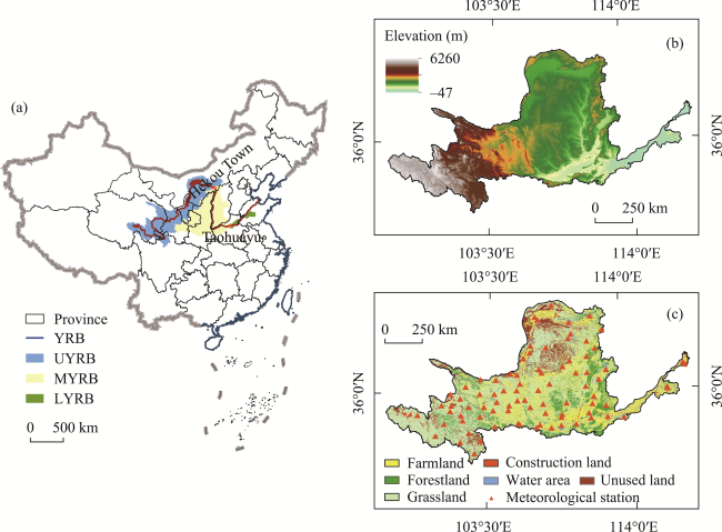
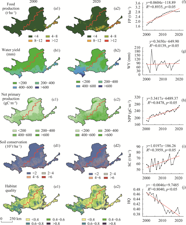
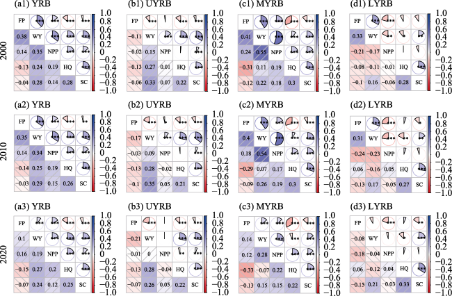
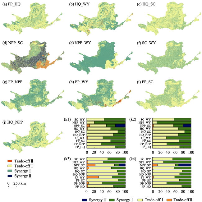
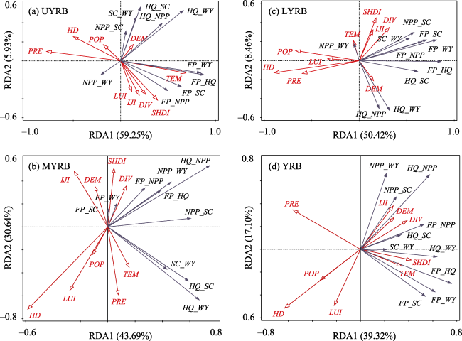
The Yellow River Basin (YRB) occupies an important position in China’s socioeconomic development and ecological conservation efforts. Understanding the spatiotemporal characteristics of the relationships among multiple ecosystem services (ESs) and their drivers is crucial for regional sustainable development and human-earth system coordination. This study simulated food production (FP), water yield (WY), net primary production (NPP), soil conservation (SC), and habitat quality (HQ) in the YRB from 2000 to 2020, and evaluated the spatial evolution and the relationship of ESs at the raster scale. Redundancy analysis was used to identify the impact of natural, socioeconomic, and landscape patterns on the relationship between ESs. The results demonstrated that the average HQ per unit area decreased by 18.10%, while SC, NPP, WY, and FP increased by 42.68%, 47.63%, 30.82%, and 67.10%, respectively, from 2000 to 2020. The relationship between ESs in the YRB was dominated by weak trade-offs and weak synergies at a temporal scale, with the trade-offs strengthened in the Upper Yellow River Basin (UYRB) and the Middle Yellow River Basin (MYRB), and synergies strengthened in the Lower Yellow River Basin (LYRB). At the spatial scale, the relationships between HQ and WY, HQ and SC, HQ and NPP, FP and SC, and FP and HQ were all dominated by trade-offs, while other ES pairs were mostly based on synergistic relationships. In the YRB, the relationships among ESs were mainly influenced by human disturbance, precipitation, and land-use and exploitation intensity. Specifically, the trade-offs among ESs in the UYRB were primarily affected by precipitation, and those in the MYRB and LYRB by human disturbance. The heterogeneity of the landscape could also effectively promote synergies among ESs. This study could provide insights into trade-offs and synergies among ESs and their driving forces and lay a foundation for ecological restoration and sustainable development of ESs in the YRB.

Cite this article

SHAO Yajing , LIU Yansui , LI Yuheng , YUAN Xuefeng . Regional ecosystem services relationships and their potential driving factors in the Yellow River Basin, China[J]. Journal of Geographical Sciences, 2023 , 33(4) : 863 -884 . DOI: 10.1007/s11442-023-2110-1

1 Introduction

Since the 20th century, problems such as global warming, food crises, water shortages, rural impoverishment, biodiversity reduction, and land desertification have occurred frequently (Eliasson, 2015; Liu and Li, 2017; Salehi, 2022). China feeds 20% of the world’s population based on only 9% of the world’s cultivated land, and the conflict between social development and ecological protection is marked (Liu et al., 2005; Liu et al., 2021). The imbalance of the human-earth relationship exacerbates the degradation of ecosystems and the loss of biodiversity, and even threatens the sustainable development of human society (Liu et al., 2020). ESs are the benefits and well-being that people derive from natural ecosystems and serve as a bridge between natural and social ecosystems (Costanza et al., 1997; Fu et al., 2015; Peng et al., 2017). Protecting, restoring, and promoting the sustainable use of terrestrial ecosystems is one of the 17 United Nations Sustainable Development Goals (SDGs) (Cord et al., 2017; Gong et al., 2019; Hu et al., 2021). Ignoring the trade-offs and synergies between ESs may threaten ecosystem security and stability (Haase et al., 2012; Morán-Ordóez et al., 2020). Therefore, understanding the spatiotemporal characteristics of ecosystem services and their relationships under the influence of multiple factors is crucial for regional sustainable development and human-earth system coordination.
Scholars have conducted many practical explorations on the relationship between ESs (Costanza et al., 2017; Nguyen et al., 2018). The research objects involve vegetation, grassland, forest, farmland, and wetland ecosystems (Wu et al., 2017; Morán-Ordóez et al., 2020; Wang et al., 2020; Fei et al., 2021; Guo and Liu, 2022). Various methods, such as the correlation coefficient method, spatial overlay method, ecosystem service trade-off degree model, root mean square error method, and production possibility frontier method, have been used to quantify the interactions among ESs (Bradford and D’Amato, 2012; Yang et al., 2015; Tomscha and Gergel, 2016; Li et al., 2018; Gong et al., 2019). The spatial heterogeneity of the natural geographical environment leads to spatial differences in the relationships between ESs (Su and Fu, 2013; He et al., 2020). For example, in Zimbabwe, South Africa, a synergy relationship existed between water yield (WY) and net primary production (NPP), while in the Fynbos Biome in Cape Town, the southernmost province of South Africa, WY and NPP mainly exist in a trade-off relationship (Chisholm, 2010; Chawanji et al., 2018). The relationship between NPP and soil conservation (SC) in the karst region of southwest China shows synergy, while in the Loess Plateau region it shows trade-offs (Wei et al., 2017; Ran et al., 2020). Due to geographic differences and human activity interference, the trade-offs and synergies between ESs are unevenly distributed in space and vary over time and space (Qiao et al., 2019; Chen et al., 2022). Existing literature has mostly focused on the spatial heterogeneity of the relationship between ESs while ignoring the evolutionary characteristics at the temporal scale, and the driving mechanisms have not been fully explored. Therefore, identifying the temporal evolution and spatial heterogeneity characteristics of trade-offs and synergies among ESs facilitates deepening our understanding of the process of anthropogenic interference with ecosystems.
Numerous studies have shown that regional environmental conditions, natural resource endowments, landscape patterns, and socioeconomic development can determine the relationships between ESs (Bennett et al., 2010; Zhang et al., 2020; Gao and Zuo, 2021). Topography is the basic geographical element that determines the ecological landscape pattern and the distribution of human activities (Hou et al., 2020). Climatic conditions determine the landscape type and configuration (Wang et al., 2020). Rural transformation, urbanization and human activities are key indicators of socioeconomic development and directly influence land use patterns and the extent of utilization (Liu et al., 2019; Han et al., 2020; Tian et al., 2020). Some studies also explored the impact of the implementation of China’s environmental protection policies, such as the Grain for Green Project, Natural Forest Conservation Program, and Prohibition of Grazing and Cutting, on the relationships between ESs (Huang et al., 2019; He et al., 2020; Hu et al., 2021). These studies laid the foundations for further analysis of ES relationships. However, previous studies were more inclined to analyze the influence of natural and socioeconomic factors, and few studies have addressed landscape factors. The comprehensive consideration of multi-factor interaction and human-earth system coupling was obviously insufficient. Landscape characteristics can reflect the influence of people’s activities on land use, potentially affecting multiple ecosystem service functions and positively or negatively affecting the relationships among ESs (Qiu and Turner, 2016; Bai et al., 2020). Therefore, analyzing the mechanisms of natural, socioeconomic, and landscape ecological influences on these relationships can provide a clearer perception of the formation mechanisms of the relationships among ESs and effectively avoid unwise management decisions due to misunderstandings.
The Yellow River Basin (YRB) is an essential ecological barrier, grain production base, and economic zone in China (Lu and Sun, 2019; Geng et al., 2022). As an ecologically fragile area in China and even in the world, problems such as the incongruity of water and sand and the imbalance of water resources seriously restrict the development of the YRB (Wang et al., 2016). Long-term anthropogenic deforestation and steep slope farming have led to the deterioration of the ecological environment in the YRB (Yang et al., 2010; Lu and Sun, 2019). In 2019, China announced the ecological protection and high-quality development of the Yellow River Basin as a major national strategy. Considering the differences in natural resources and socioeconomic development in the upper, middle, and lower reaches of the YRB, exploring the trade-offs and synergies relationships and their driving mechanisms is of practical guidance for the sustainable development of the YRB. Against this background, three aspects were of interest in this study: (1) How did multiple ESs change from 2000 to 2020? (2) What are the characteristics of trade-offs and synergies between ESs at the temporal and spatial scales? (3) Are there significant regional differences in the response of ES trade-offs and synergies to drivers in different regions of the YRB? The results are expected to provide theoretical and technical support for decision-makers to develop differentiated ecological management strategies and high-quality development paths in the YRB.

2 Materials and methods

2.1 Study area

The Yellow River Basin (YRB) originates from the Qinghai-Tibet Plateau, between 32°-42°N and 96°-119°E. The total length of the mainstream of the YRB is 5464 km. The YRB has a total area of 79.5 × 10⁴ km2 (including 4.2 × 10⁴ km2 of internal flow area) (Wang et al., 2004). The YRB spans different geographical units, including the Qinghai-Tibet Plateau, Mongolian Plateau, Loess Plateau, and North China Plain from west to east. The terrain of the YRB is high in the west and low in the east (Figure 1). Hekou Town in Inner Mongolia and Taohuayu in Henan Province are the demarcation points between the upper, middle, and lower reaches of the YRB, respectively (Yang et al., 2010). The YRB has a continental climate, with semi-humid, semi-arid, and arid climates from southeast to northwest and an average annual precipitation of 200-600 mm.
Figure 1 Location of the Yellow River Basin (a), DEM (b), and land-use pattern (c)
According to the Comprehensive Planning of the Yellow River Basin (2012-2030), the YRB flows through the following nine provincial-level regions (hereafter province): Qinghai, Sichuan, Gansu, Ningxia, Inner Mongolia, Shanxi, Shaanxi, Henan, and Shandong. In 2020, the total population of the nine provinces accounted for 29.82% of the total population of China. The GDP of these provinces accounted for about 1/4 of the GDP of China. As an important ecological barrier area, the YRB plays a global and strategic role in China’s economic development and ecological protection.

2.2 Data sources and preparation

Table 1 shows the datasets used in this study. To unify the research scale, all spatial data were unified to the same spatial reference, the projection coordinate was unified as Krasovsky_1940_Albers, and the resolution was unified as 250 m.
Table 1 Datasets sources and descriptions
Category Data sources and description Data source
Land-use/cover dataset Raster data, 30 m × 30 m Resource and Environment Science and Data Center, Chinese Academy of Sciences (http://www.resdc.cn)
Meteorological data Site China Meteorological Science Data Center (http://data.cma.cn/)
Digital elevation model (DEM) Raster, 90 m × 90 m Geospatial Data Cloud (http://www.gscloud.cn/)
Normalized Difference
Vegetation Index (NDVI)
Raster, 250 m × 250 m Geospatial Data Cloud (http://www.gscloud.cn/)
Soil data (soil type, soil texture, soil organic matter content, and root depth) Vector Harmonized World Soil Database V1.2 provided by the Cold and Arid Regions Science Data Center at Lanzhou (http://www.fao.org/soils-portal/soil-survey/soil-maps-and-databases/ harmonized-world-soil-database-v12/en/)
Socioeconomic data Raster, 1000 m × 1000 m Chinese Academy of Sciences Resources Environment Science and Data Center (http://www.resdc.cn/)
Statistical data Statistical Yearbook of nine provincial-level regions distributed along the YRB

2.3 Research methods

2.3.1 Quantification of ecosystem services

(1) Food Production (FP)
FP has a linear relationship with the Normalized Difference Vegetation Index (NDVI) (Potdar et al., 1995; Pereira, 2017). This study draws on the research of Wu et al. (2017) to spatialize and rasterize the FP on the foundation of the NDVI distribution. The specific formula is as follows:
$F{{P}_{i}}=\frac{NDV{{I}_{i}}}{NDV{{I}_{sum}}}\times {{P}_{sum}}$
where FPi is the output of grain, livestock, or aquatic products of the ith grid. Psum is the output of grain, livestock, or aquatic products of the city where the ith raster is located (t·ha‒1·a‒1); NDVIi is the NDVI of the ith grid of farmland or grassland or water area; NDVIsum is the sum of NDVI of farmland, grassland, or water area in the study area.
(2) Water yield (WY)
The annual WY module of the InVEST model version 3.6.0 is applied to estimate the total and average volume of WY. The model is based on the Budyko curve and the regional annual. Y is equal to the difference between annual precipitation and actual evapotranspiration (Budyko, 1974). The basic principles of the model are as follows:
$Y(x)=\left( 1-\frac{AET(x)}{P(x)} \right)\times P(x)$
where Y(x), AET(x), and P(x) are the annual WY (mm), actual annual evapotranspiration (mm), and annual precipitation (mm) of grid x, respectively.
$\frac{AET(x)}{P(x)}=1+\frac{PET(x)}{P(x)}-{{\left[ 1+{{\left( \frac{PET(x)}{P(x)} \right)}^{w}} \right]}^{1/w}}$
$PET(x)={{K}_{c}}({{l}_{x}})\times E{{T}_{0}}(x)$
$w(x)=\frac{Z\times AWC(x)}{P(x)}+1.25$
$AWC=\min ({{D}_{s}}/{{D}_{r}})\times PAWC$
$\begin{align} & PAWC=54.509-0.132\times SAND-0.003\times SAN{{D}^{2}}-0.055\times SILT \\ & -0.006\times SIL{{T}^{2}}-0.738\times CLAY+0.007\times CLA{{Y}^{2}}-2.688\times OM+0.501\times O{{M}^{2}} \\ \end{align}$
$Z=0.2N$
where PET(x) is the annual potential evapotranspiration (mm) of grid x, w(x) is a non-physical parameter of natural climate-soil properties; an empirical parameter. ET0(x) is the reference evapotranspiration of grid x, which is calculated by ET0 Calculator V32. Kc (lx) is the plant transpiration and evaporation coefficient of a specific land-use type in grid x, computed using the kc calculator provided by FAO. PAWC is the available water content of vegetation; SAND, SILT, CLAY, and OM represent the percentage content of soil sand, soil silt, soil clay, and soil organic matter content, respectively. Ds (mm) is the depth of soil, and Dr (mm) is the root depth. Z is an empirical constant reflecting local hydrological conditions (Zhang et al., 2004). N represents the number of days of rainfall in a year (> 1 mm) (Donohue et al., 2012).
(3) Soil conservation (SC)
The SC can be quantified by the Revised Universal Soil Loss Equation (Renard et al., 1997), calculated as follows:
$SC=R\times K\times LS\times (1-C\times P)$
where SC is the amount of soil conservation (t/ha·year). R is the rainfall erosion factor (MJ·mm/ha·h·a), calculated according to the formula proposed by Wischmeier and Smith (1958). K is the soil erodibility factor (t·ha·h/(ha·MJ·mm)), calculated by the EPIC model proposed by Sharpley and Williams (1990). LS is a topographic factor calculated by the soil erosion model topographic factor calculation tool (2.0) provided by the National Earth System Science Data Center. C is the vegetation cover and management factor, dimensionless, calculated according to the method proposed by Cai et al. (2000). P is the conservation support practice factor, dimensionless, calculated referring to Lufafa et al. (2003).
(4) Net Primary Production (NPP)
The CASA (Carnegie Ames-Stanford Approach) model is used to calculate NPP in the YRB (Potter et al., 1993; Liu et al., 2019). The basic principles of the model are as follows:
$NPP(x,t)=APAR(x,t)\times \text{ }\!\!\varepsilon\!\!\text{ }(x,t)$
$APAR(x,t)=SOL(x,t)\times FPAR(x,t)\times 0.5$
$\text{ }\!\!\varepsilon\!\!\text{ }(x,t)={{\text{T}}_{\text{ }\!\!\varepsilon\!\!\text{ }1}}(x,t)\times {{T}_{\text{ }\!\!\varepsilon\!\!\text{ }2}}(x,t)\times {{W}_{\text{ }\!\!\varepsilon\!\!\text{ }}}(x,t)\times {{\text{ }\!\!\varepsilon\!\!\text{ }}_{\max }}$
$FPAR(x,t)=\min \left( \frac{SR(x,t)-S{{R}_{\min }}}{S{{R}_{\max }}-S{{R}_{\min }}},0.95 \right)$
$SR(x,t)=\frac{1+NDVI(x,t)}{1-NDVI(x,t)}$
where NPP(x, t) is the net primary productivity (gC/(m2·a) of grid x at t-month. APAR(x, t) refers to the photosynthetically active radiation (MJ/m2) by grid x in t-month. ε(x, t) is the actual light use efficiency (gC/MJ) of grid x at t-month. SOL(x, t) is the total solar radiation (MJ/m2) of grid x in t-month. FPAR(x, t) is the absorption ratio of incident photosynthetic active radiation by vegetation layer (dimensionless). Tε1(x, t) and Tε2(x, t) are the influence coefficients of low temperature and high temperature on vegetation’s light energy utilization efficiency, respectively. Wε(x, t) represents the water stress coefficient (dimensionless). εmax is the maximum light energy utilization efficiency of vegetation in an ideal condition (gC/MJ). SR (x, t) is the vegetation coefficient ratio of grid x in month t, SRmin and SRmax are the 95% and 5% side percentiles of NDVI for each vegetation type, respectively.
(5) Habitat quality (HQ)
The habitat quality model of the InVEST model is used to assess the HQ of the YRB. The basic principles of the model are as follows:
${{Q}_{xj}}={{H}_{j}}\left( 1-\left( \frac{D_{ij}^{z}}{D_{ij}^{z}+{{K}^{z}}} \right) \right)$
${{D}_{ij}}=\sum\limits_{r=1}^{R}{\sum\limits_{y=1}^{{{Y}_{r}}}{\left( \frac{{{W}_{r}}}{\sum\nolimits_{r=1}^{R}{{{W}_{r}}}} \right)}}{{r}_{y}}{{i}_{rxy}}{{\text{ }\!\!\beta\!\!\text{ }}_{x}}{{S}_{jr}}$
where Qxj is the HQ of land-use type j in raster x; Dxj is the total threat level of land-use type j in raster x; R is the number of threats; Yr is the grid number of threats r; Wr is the weight of threat r, with a value between 0 and 1; ry is the threat value of grid y; irxy is the impact of threat r on the habitat in grid x; βx is the accessibility in grid x; Sjr is the sensitivity of habitat type j to stress factor r; K and Z are proportional factors; Hj is the habitat suitability of land-use type j. In this study, we took farmland, construction land, and roads as threat sources, and the setting of parameters such as the influence distance and the sensitivity of threat factors mainly refers to the research of Fu et al. (2020) and Shui et al. (2018).

2.3.2 Theil-Sen median trend analysis and Mann-Kendall test

Theil-Sen median trend analysis, also known as Sen slope estimation, is a robust trend calculation method for nonparametric statistics (Fensholt et al., 2012). The Theil-Sen median is used to assess the changing trend of ecosystem services on the cell scale. The calculation formula is as follows:
$\text{ }\!\!\beta\!\!\text{ }=\text{m}edian\left( \frac{{{x}_{j}}-{{x}_{i}}}{j-i} \right),\forall j>i$
where β is the changing trend of the ESs; xi and xj are ESs at i and j time, respectively. When β>0, ESs are increasing, conversely, β < 0, ESs are decreasing.
Since Theil-Sen median trend analysis cannot make a significant judgment on the trend of geographic elements changing in the time series, it is also necessary to combine the Mann-Kendall method to test the significance of the trend (Liu et al., 2015). The calculation formula is as follows:
$Z=\left\{ \begin{matrix} \begin{matrix} \frac{S-1}{\sqrt{Var(S)}} \\ 0 \\ \frac{S+1}{\sqrt{Var(S)}} \\ \end{matrix} & \begin{matrix} S>0 \\ S=0 \\ S<0 \\ \end{matrix} \\ \end{matrix} \right.$
$S=\sum_{i=1}^{n-1} \sum_{j=i+1}^{n} \operatorname{sgn}\left(E T_{j}-E T_{i}\right)$
$\operatorname{sgn}\left(E T_{j}-E T_{i}\right)=\left\{\begin{array}{cc}1 & E T_{j}-E T_{i}>0 \\0 & E T_{j}-E T_{i}=0 \\-1 & E T_{j}-E T_{i}<0\end{array}\right.$
$V\text{ar}(S)=\frac{n(n-1)\text{ }(2n+5)}{18}$
where n is the length of the time series, and given a significance level a, when |Z| > Z1-a/2, the data show a significant change during the study period at the a level. When |Z| > 1.96, it indicates that the change trends are significant, when |Z| ≤ 1.96, it indicates that the change trends are not significant.

2.3.3 Measuring the trade-offs and synergies among ESs

(1) Correlation coefficient method
Pearson correlation analysis was used to analyze the overall characteristics of the trade-offs and synergies between ESs (Long et al., 2018; Chen et al., 2022). Before conducting Pearson correlation analysis, we sampled ESs with sample points at equal intervals of 10 km. The correlation analysis was implemented through the R language package.
${{R}_{xy}}=\frac{\sum\nolimits_{i=1}^{n}{\left[ ({{x}_{i}}-\bar{X})({{y}_{i}}-\bar{Y}) \right]}}{\sqrt{\sum\nolimits_{i=1}^{n}{{{({{x}_{i}}-\bar{X})}^{2}}\sum\nolimits_{i=1}^{n}{{{({{y}_{i}}-\bar{Y})}^{2}}}}}}$
where Rxy is the correlation coefficient between features x and y, n is the sample size,$\bar{X}$and $\bar{Y}$represent the means of x and y, xi and yi are the i-th year values of x and y, respectively. Rxy > 0, Rxy < 0, and Rxy = 0 indicate synergistic trade-off, and no-relation between x and y, respectively.
(2) Ecosystem service trade-offs and synergies degree index (ESTD)
The ESTD can reflect the interaction and extent between ESs and can be used to reveal the spatial heterogeneity of the trade-offs and synergies between ESs (Gong et al., 2019). If the ESTD value is positive, it means that the two ESs are in a synergistic relationship. Otherwise, it is a trade-off relationship. ESTD is calculated as follows:
$EST{{D}_{ij}}=\frac{(E{{S}_{ia}}-E{{S}_{ib}})/E{{S}_{ib}}}{(E{{S}_{ja}}-E{{S}_{jb}})/E{{S}_{jb}}}$
where ESTDij is the trade-offs and synergistic relationship between the ith and jth ES; ESia and ESja are the value of ith and jth ES at time a; ESib and ESjb are the value of ith and jth ES at time b, respectively; and a and b represent the end and start of the study period.

2.3.4 Selection and quantification of influencing factors

(1) Selection of influencing factors
Based on the availability of data, we selected 12 factors from natural, socioeconomic, and landscape perspectives, among which natural factors include the Digital Elevation Model (DEM), Temperature (TEM), and Precipitation (PRE); socioeconomic factors include population density (POP), land-use and exploitation intensity (LUI), and human disturbance index (HD); landscape factors include the Interspersion and Juxtaposition index (IJI), Division (DIV), and Shannon’s Diversity Index (SHDI).
Among the influencing factors, the data sources of DEM, TEM, PRE, and NDVI are detailed in section 2.2. LUI reflects the intensity of development and utilization of land resources, which can be expressed as a percentage of the area of construction land. HD can characterize the impact of human activities on ecosystem services, and its calculation can refer to existing studies (Han et al., 2020). The landscape index was also quantified by Fragstats 4.2.
(2) Redundancy analysis (RDA)
RDA is a ranking method of multiple linear regression combined with principal component analysis, which can reveal the relationship between univariate and multivariate or multivariate and multivariate (Legendre, 2008). The results of RDA are displayed in a two-dimensional form on the ranking diagram, and the relationship between explanatory and explained variables can be visualized in a low-dimensional space (Dai et al., 2020; Dou et al., 2020). The angle between the arrows represents the correlation between the variables. If the angle is acute, the smaller the angle, the stronger the positive correlation between the two variables. If the angle is a right angle, it means that the two variables are almost unrelated. If the angle is obtuse, the larger the angle, the stronger the negative correlation between the variables (Jaligot et al., 2019). The Monte Carlo permutation test is used to show whether the explanation of driving forces on the response variables is significant. The RDA was implemented using CANOCO for Windows v5.0. The relationship between ES pairs was the dependent variable, and the natural-socioeconomic-landscape index was the independent variable. All data were normalized and sampled using a 10 km grid before performing the RDA analysis.

3 Results

3.1 Spatiotemporal variation of ESs in the YRB

From 2000 to 2020, the average HQ per unit area in the YRB decreased by 18.10%, while the SC, NPP, WY, and FP increased by 42.68%, 47.63%, 30.82%, and 67.10%, respectively (Figures 2f-2j). Overall, the spatial distribution pattern of five ESs presented as “low in the north and high in the south” (Figures 2a1-2e2). The high-value areas of FP were mainly distributed in the Kuan-chung Plain of the Middle Yellow River Basin (MYRB) and in the North China Plain of the Lower Yellow River Basin (LYRB). The high-value areas of WY were located in Qinghai in the Upper Yellow River Basin (UYRB). The spatial distribution characteristics of NPP and SC were relatively similar, with the high-value areas mainly concentrated in the MYRB and LYRB. The high-value areas of HQ were mainly concentrated in the UYRB and MYRB.
Figure 2 Spatial distribution (a1-e2) and temporal variation (f-j) of five ESs in the Yellow River Basin from 2000 to 2020
According to the results of the Theil-Sen median trend analysis and Mann-Kendall test (Figure 3), NPP, WY, FP, and SC in the YRB were dominated by increasing trends, while from 2000 to 2020, HQ was mainly dominated by decreasing trends. The areas with a non- significant and significant increase of WY accounted for 63.43% and 17.52% of YRB, respectively, among which the areas with significant increases were mainly located in Guyuan, Qingyang, and Pingliang cities in the MYRB, and the Tibetan Autonomous Prefecture of Hainan, Huangnan, and Golog in the UYRB. The spatial evolution of NPP has obvious regional differences, with significantly increased areas accounting for 31.27% of the YRB, mainly concentrated in the MYRB, and non-significantly increased areas accounting for 66.12% of the YRB, mainly distributed in the UYRB and LYRB. SC and FP were both dominated by non-significant increases, accounting for 62.52% and 63.61% of the YRB, respectively, and were mainly distributed in the MYRB and UYRB. The FP in the Kuan-Chung Plain in the MYRB and the North China Plain in the LYRB showed a significant increasing trend, while the SC showed a non-significant decreasing trend. The HQ in 84.82% area of the YRB showed a non-significant decreasing trend, but Yan’an, Yulin, and Qingyang cities in the MYRB, located in the Loess Plateau, showed a non-significant increasing trend.
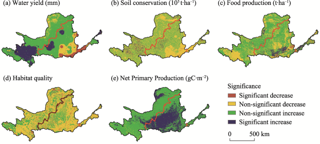
Figure 3 Spatial evolution trends of ESs in the Yellow River Basin from 2000 to 2020

3.2 Trade-offs and synergies of ESs

3.2.1 Temporal variation characteristics of trade-offs and synergies among ESs

Pearson’s correlation coefficients were used to analyze the trade-offs and synergistic relationships among ESs, and the correlation coefficients were classified as highly correlated (|r| ≥ 0.5), moderately correlated (0.3 ≤ |r| < 0.5), and weakly correlated (|r| < 0.3). There are two pairs of trade-offs and eight pairs of synergies in the YRB, and the trade-offs and synergies among 10 pairs of ESs were significant, with correlation coefficients mainly in the range of 0-0.3 (Figure 4).
Figure 4 Pearson correlation between ES pairs in the Yellow River Basin (a), UYRB (b), MYRB (c), and LYRB (d) (Blue and red pies show positive and negative correlations, respectively. Significance levels are *p < 0.05, **p < 0.01, ***p < 0.001.)
In the UYRB, trade-offs exist among FP and WY, FP and NPP, FP and HQ, and FP and SC, and synergies exist among WY and HQ, WY and SC, HQ and SC, and NPP and SC. The synergistic relationship between WY and NPP gradually weakened, and the relationship between NPP and HQ changed from a synergistic relationship to a trade-off relationship. In the MYRB, there are trade-offs between FP and HQ, and FP and SC, and synergies between the other eight pairs of ESs. The relationship between WY and HQ has shifted from synergy to trade-off. In the LYRB, there are trade-offs between FP and NPP, WY and NPP, WY and HQ, NPP and SC, and FP and SC, and synergies between HQ and SC, and WY and SC. The trade-off between FP and HQ, and NPP and HQ weakened while the synergistic relationship increased, and the synergies between FP and WY weakened. In terms of the evolution trends of ES relationships, the trade-offs strengthened while the synergies weakened in UYRB and MYRB. However, the synergies strengthened and trade-offs weakened in the LYRB.

3.2.2 Spatial characteristics of trade-offs and synergies between ESs.

In this study, the ESTD results were classified into four levels through the natural break-point method, including strong trade-off (trade-off II), weak trade-off (trade-off I), strong synergy (synergy II), and weak synergy (synergy I). Among the 10 pairs of ESs, from 2000 to 2020, NPP and WY, FP and NPP, FP and WY, SC and WY, and NPP and SC mainly showed synergistic relationships in the YRB, while other ES pairs were dominated by trade-off relationships. More than 70% of the area in the YRB presented trade-offs between HQ and SC, FP and HQ, and HQ and NPP (Figure 5).
Figure 5 Trade-offs and synergies among ESs in the Yellow River Basin from 2000 to 2020 (k1, k2, k3, and k4 represent the YRB, UYRB, MYRB, and LYRB, respectively.)
The relationships among ESs in the YRB were dominated by weak trade-offs and weak synergies. Compared with other ES pairs, the areas with strong trade-offs and strong synergies between NPP and SC were widely distributed in the YRB, accounting for 8.23% and 21.11% of the YRB area, respectively, while the areas with strong synergy were mainly distributed in Haidong, Xining, and Huangnan in Qinghai, Dingxi, Lanzhou, Linxia, Qingyang, and Pingliang in Gansu, Yulin, and Yan’an in Shaanxi, and Lvliang and Linfen in Shanxi. The areas that showed a strong trade-off relationship were mainly distributed at the junction of Shanxi, Shaanxi, and Henan provinces, including Weinan and Xi’an in Shaanxi, Luoyang in Henan, and Jincheng in Shanxi.

3.3 Driving mechanism of ESs’ trade-offs and synergies

Before performing the redundant analysis, detrended correspondence analysis (DCA) was used to determine whether to choose a linear model or a single peak model. The DCA gradient length values in the YRB, UYRB, MYRB, and LYRB were 2.6, 2.7, 2.2, and 2.8, respectively. They were all less than 3, indicating that the RDA model is more appropriate for revealing the influencing factors of the trade-offs and synergies among ESs. In the RDA analysis, the results of the full-axis Monte Carlo tests in the YRB, UYRB, MYRB, and LYRB were 0.002, 0.002, 0.002, and 0.004 (p < 0.05), respectively, indicating that there were statistically significant relationships between the trade-offs and synergies of 10 ESs pairs and drivers in different regions of the YRB.
The results of RDA showed that the nine factors could explain 61.8% (adjusted R2 = 50.4%), 74.9% (adjusted R2 = 53.1%), 81.3% (adjusted R2 = 64.6%), and 63.3% (adjusted R2 = 43.3%) of the trade-offs and synergistic relationships between the ESs in the YRB, UYRB, MYRB, and LYRB, respectively (Table 2). The statistics on the interpretation degree of the driving factors from the perspective of natural, economic, and landscape patterns showed that the trade-offs and synergies among ESs in the YRB were mainly affected by socioeconomic factors, and the interpretation rate reached 32.7%. Comparing different regions of the YRB, natural factors were the dominant factors in the relationship between ESs in the UYRB, with an explanation degree of more than 40%, and socioeconomic factors were the dominant factors in the relationship between ESs in the MYRB and LYRB, with interpretation rates of 39.5% and 35%, respectively.
Table 2 The percentage of variance explained by drivers in the YRB (p < 0.001)
Drivers YRB UYRB MYRB LYRB
Percentage of variance explained F-value Rank Percentage of variance explained F-value Rank Percentage of variance explained F-value Rank Percentage of variance explained F-value Rank
DEM 2.00 1.10 8 1.80 0.60 9 3.10 0.90 8 2.50 0.50 8
PRE 13.20 7.00 2 35.40 16.60 1 14.30 5.30 2 10.50 2.40 2
TEM 1.70 0.40 9 7.40 8.20 3 4.40 2.20 6 2.20 0.30 9
LUI 10.60 5.30 3 2.20 1.00 8 7.50 3.10 4 3.80 0.90 6
POP 6.20 3.80 4 2.50 1.10 7 2.20 0.60 9 9.60 2.20 3
HD 15.90 10.80 1 5.10 3.50 4 29.80 12.00 1 21.60 20.60 1
IJI 5.20 3.60 5 3.20 1.50 6 7.20 3.10 5 3.20 0.60 7
DIV 4.80 1.90 6 3.50 1.80 5 3.60 1.60 7 4.40 1.60 5
SHDI 2.20 1.50 7 13.80 2.40 2 9.20 1.70 3 5.50 1.70 4
Total 61.80 / / 74.90 / / 81.30 / / 63.30 / /
The cumulative variance percentages of the two axes in the YRB, UYRB, MYRB, and LYRB were 56.42%, 65.18%, 74.33%, and 58.88% respectively. Therefore, the first two principal components could explain more than 50% of the heterogeneity of trade-offs and synergies among ESs (Figure 6). In the YRB (Figure 6d), HD, PRE, and LUI were the main drivers of the trade-offs and synergies among ES pairs. The influence of drivers varied widely in different regions of the YRB. For natural factors in the UYRB (Figure 6a), an increase in PRE would increase the intensity of trade-offs between FP and WY, FP and HQ, FP and SC, and FP and NPP. Conversely, an increase in TEM would intensify the synergies between these service pairs. In the MYRB (Figure 6b), PRE has a correlation with TEM, and the increase in PRE and TEM could strengthen the synergies between SC and WY, HQ and SC, and HQ and WY, and also intensify the trade-offs between FP and WY, FP and HQ, FP and SC, and FP and NPP. In the LYRB, the increase in PRE (Figure 6c) could intensify the trade-offs between all ESs. In terms of socioeconomic factors, HD has the most significant influence on the trade-offs among ESs in the YRB, especially in the MYRB and LYRB, where HD explained 29.8% and 21.6% of the relationships between ESs, respectively. Among socioeconomic factors, there was a high correlation between HD and POP, and their increase could exacerbate the trade-offs between ES pairs, especially between FP and other services. As for landscape factors, SHDI, DIV, and IJI have a positive impact on the synergistic relationship between most ES pairs in the YRB. The increase in SHDI, IJI, and DIV could increase the synergies between FP and other services in the UYRB, the synergies between FP and SC, FP and WY, and FP and NPP in the MYRB, and the synergistic relationship between SC and WY, SC and NPP, and SC and FP in the LYRB.
Figure 6 Redundancy analysis of the ES relationships and driving factors in the Yellow River Basin

4 Discussion

4.1 Spatiotemporal characters in trade-offs and synergies among ESs and the driving factors

Our findings show that the trade-offs and synergies among multiple ESs (FP, NPP, SC, WY, HQ) in the YRB are significantly spatially heterogeneous, consistent with Li et al. (2018). The environmental condition, natural resource endowment, and socioeconomic development lead to variability in the type and intensity of ESs in different regions. In the YRB, FP and WY are mainly in a synergistic relationship in the plateau areas in the UYRB, while they are in a trade-off relationship in the plain areas in the MYRB and LYRB, also confirming the research of Li et al. (2017; 2018). The relationship between FP and WY is often closely related to the amount of rainfall and the development of agricultural production (Dou et al., 2020). The uneven rainfall leads to the spatial heterogeneity of WY in the YRB (Geng et al., 2022). The UYRB is located in arid and semi-arid areas, and agricultural production is more dependent on water production services, implying that there may be synergies between FP and WY. However, in the LYRB and MYRB, China’s main grain production base, the competition between FP and WY is more significant.
The trade-offs and synergies between ESs may change over different periods (Rodríguez et al., 2006). The findings of the correlation analysis identify weak trade-offs and synergies among ESs in the YRB. From 2000 to 2020, in the UYRB and MYRB, the synergies were weakening while the trade-offs were strengthening. However, the synergies were strengthening in the LYRB. Previous studies showed that if the trade-offs and synergistic relationships between ESs were weak, trade-offs and synergy relationships could very easily develop inter-conversion (Li et al., 2018). The evolution of relationships between ESs is often related to regional natural conditions and socioeconomic development. In the UYRB, the relationships between NPP and HQ shifted from synergies to trade-offs, mainly due to pasture degradation and reduced vegetation cover. In the MYRB, especially in the Loess Plateau region, there is a clear greening trend (Cao et al., 2018; He et al., 2020). The increase in vegetation cover significantly improved the HQ, but also increased regional surface evaporation, causing a decline in WY, resulting in a gradual strengthening of the trade-off between HQ and WY. In the LYRB, with the progress of science and technology and the construction of ecological civilization, the relationship between FP and HQ has gradually changed from trade-offs to synergies.
The impact of drivers on the trade-offs and synergies among ESs varied in different regions of the YRB. Xu et al. (2020) found that the relationship between ESs was closely related to regional climate, altitude, population, and other factors, among which human activities were the most significant. Our results found that HD was the main factor leading to the trade-offs and synergies between ESs in the YRB, especially in the MYRB and LYRB. Furthermore, numerous studies have confirmed that increases in population and changes in land-use structure and intensity caused changes in the structure and function of ESs (Liu et al., 2014; Bai et al., 2020; Hou et al., 2020; Liu et al., 2022). It is noteworthy that the landscape factors (IJI, DIV, SHDI) could promote the synergies between FP and other services in the UYRB, MYRB, and LYRB, and this implies that the heterogeneity of the landscape has a positive impact on the synergistic relationship between ESs to some extent. We also found that an increase in precipitation could intensify the synergies between HQ and SC in the MYRB, and the trade-offs between HQ and SC in the LYRB. Previous studies have shown that precipitation, as the primary source of water demand for vegetation in arid and semi-arid areas, was a key factor affecting regional SC (Hou et al., 2020; Zhu et al., 2020). The increase in rainfall could increase soil moisture and intensify regional soil erosion, but with the addition of appropriate environmental protection engineering measures, it could improve the soil retention capacity of the region (Dou et al., 2020; Geng et al., 2022). The spatial heterogeneity of trade-off and synergies among ESs requires variability in the management policies of different stakeholders for different services and the relationships among them (Zheng et al., 2019; Zhang et al., 2022).

4.2 The implications for high-quality development of the YRB

The UYRB is a typical ecologically fragile area in China, with severe water shortages, slow economic development, and limited agricultural production. Liu et al. (2017) identified that water scarcity has seriously affected the availability of freshwater resources and vegetation growth in the UYRB, resulting in a lack of endogenous power for traditional agriculture. Our study showed that the trade-offs between FP and HQ, and FP and SC are prominent in the UYRB, and increases in rainfall exacerbate trade-offs between ESs, especially between FP and other services, while increases in landscape diversity and heterogeneity have a positive impact on synergistic relationships between regional ESs. Therefore, the UYRB should strengthen the construction of water conservancy facilities and implement effective ecological restoration strategies to improve the diversity of the regional ecosystem and give full play to the multifunctional nature of the ecosystem.
The MYRB flows through the Loess Plateau area and carries a large amount of sediment. The Loess soil is loose and susceptible to climate and topographic features, so soil erosion is the greatest stressor to ecosystem services in the region (Bing et al., 2011; Cao et al., 2016; Zhang et al., 2019). In recent years, although the implementation of a series of environmental protection policies has effectively increased the regional vegetation cover, it still has not effectively improved the erosion resistance of regional soils (Jiang et al., 2016). Moreover, some studies have indicated that the increase in vegetation cover in the region may simultaneously lead to a decrease in food production services (Fu et al., 2015). We found that the trade-offs between SC and FP, SC and NPP, and SC and HQ were widely distributed in the MYRB, and the trade-off between them gradually increased under the influence of HD. The MYRB is undergoing rapid urbanization, and the pressure on the environment from population growth will continue to intensify (Zhao et al., 2021). The MYRB should adhere to the concept of green development, improve the conditions of agricultural water conservancy facilities, build wide terraces to ensure regional food security, implement ecological restoration projects to improve regional anti-erosion capacity, and scientifically determine the scale of vegetation restoration to alleviate the pressure on water resources.
The LYRB, especially the central and southern parts of the Jiaodong Peninsula, is the main area for biodiversity conservation and raw material production in the YRB. After 2000, the rapid population growth in the LYRB led to increased environmental pressure, intensifying the spatial imbalance of ESs. The decrease in farmland could reduce FP and the intensity of the trade-offs between FP and other services (Wang et al., 2012). We found that more than 70% of the area of the LYRB showed a trade-off between FP and SC, and FP and HQ. Moreover, the increase in HD, POP, and LUI will intensify the trade-off between ESs in LYRB. Improving the diversity and heterogeneity of ecological landscapes in downstream areas is conducive to promoting the synergistic relationship between ESs.

4.3 Limitations and further study

Mastering the relationships among ESs is a prerequisite for optimizing the supply of ESs and can provide the basis for territorial spatial planning, biodiversity conservation, and ecological restoration (Haase et al., 2012; Chen et al., 2022). Considering the availability of data, five services were selected and quantified using different biophysical models to characterize the ESs of the YRB. Although these five services are typical, they still do not fully reflect the overall characteristics of watershed ecosystem functions and the interaction of human-earth system. The Yellow River is the mother river of the Chinese people and the birthplace of Chinese urban civilization. Cultural services are also one of the important types of services in the YRB. In addition, the Mu Us Desert is located in the northeastern part of the YRB, and the wind and sand control function of the ecosystem cannot be ignored. Therefore, it is necessary to strengthen the quantification of ESs from multiple perspectives and use multiple sources of data in the future to comprehensively reveal the functional characteristics of the ecosystem in the YRB.
Given the complexity and comprehensiveness of ESs and the fact that the relationships among ESs also vary with the study scale and land-use scenarios, we should pay more attention to the formation mechanism and scale-dependent characteristics of ES trade-offs and synergies in different land-use contexts, predicting the evolution of trade-offs and synergistic relationships among ESs, and optimizing them with appropriate scenarios. The future management of ecosystem services should also consider the actual demand of stakeholders and the regional supply level at different spatial and temporal scales to achieve a “win-win” situation of socioeconomic development and ecological conservation under the harmonious coexistence of human and nature and the transformation of rural regional system.

5 Conclusion

This study investigated the spatiotemporal evolution characteristics of five typical ESs (FP, WY, NPP, SC and HQ) and assessed the trade-offs and synergies among ESs in the YRB. We also analyzed the driving factors of the relationships from natural, socioeconomic, and landscape perspectives. The results show that, from 2000 to 2020, in spatial and temporal scales, HQ in the YRB exhibited a decreasing trend, while FP, SC, WY, and NPP showed an increasing trend. Based on correlation analysis and the trade-offs and synergies degree index (ESTD), it was found that the relationships between ESs have changed significantly. Specifically, the relationships between NPP and HQ (in the UYRB), and WY and HQ (in the MYRB) changed from synergies to trade-offs, and the relationship between FP and HQ, and NPP and HQ changed from trade-offs to synergies in the LYRB.
ES relationships are underpinned by multiple factors, and the dominant influences differ across regions of the YRB. Overall, the relationship between ESs was primarily influenced by precipitation in the UYRB and by HD in the MYRB and LYRB. Precipitation promotes trade-offs between FP and WY, FP and HQ, and FP and SC, especially in arid and semi-arid regions. In contrast, in socio-economically developed areas, human disturbances are the main factor in the trade-offs and synergies between ESs. The findings of this study facilitate our understanding of the formation mechanisms of the trade-offs and synergies between ESs and provide a basis for regional ecological restoration, ecological compensation, and territorial spatial planning projects.
[1]
Bai Y, Chen Y, Alatalo J M et al., 2020. Scale effects on the relationships between land characteristics and ecosystem services: A case study in Taihu Lake Basin, China. The Science of the Total Environment, 716: 137083.

DOI

[2]
Bennett E M, Peterson G D, Gordon L J, 2010. Understanding relationships among multiple ecosystem services. Ecology Letters, 12(12): 1394-1404.

DOI

[3]
Bing L F, Shao Q, Liu J Y, et al., 2011. Runoff characteristics in flood and dry seasons in source regions of Changjiang River and Huanghe River based on wavelet analysis. Scientia Geographica Sinica, 31(2): 2323-2328. (in Chinese)

[4]
Bradford J B, D’Amato A W, 2012. Recognizing trade-offs in multi-objective land management. Frontiers in Ecology & the Environment, 10(4): 210-216.

[5]
Budyko M I, 1974. Climate and Life. New York: Academic Press.

[6]
Cai C F, Ding S W, Shi Z H, et al., 2000. Study of applying USLE and geographical information system IDRISI to predict soil erosion in small watershed. Journal of Soil Water Conservation, 14(2): 19-24. (in Chinese)

[7]
Cao S X, Zhang J Z, Chen L et al., 2016. Ecosystem water imbalances created during ecological restoration by afforestation in China, and lessons for other developing countries. Journal of Environmental Management, 183: 843-849.

DOI PMID

[8]
Cao Z, Li Y R, Liu Y S et al., 2018. When and where did the Loess Plateau turn “green”? Analysis of the tendency and breakpoints of the normalized difference vegetation index. Land Degradation & Development, 29(1): 162-175.

DOI

[9]
Chawanji S, Masocha M, Dube T, 2018. Spatial assessment of ecosystem service trade-offs and synergies in Zimbabwe. Transactions of the Royal Society of South Africa, 73(2): 1-8.

DOI

[10]
Chen T T, Peng L, Wang Q, 2022. Response and multiscenario simulation of trade-offs/synergies among ecosystem services to the Grain to Green Program: A case study of the Chengdu-Chongqing urban agglomeration, China. Environmental Science and Pollution Research, 29(22): 33572-33586.

DOI

[11]
Chisholm R A, 2010. Trade-offs between ecosystem services: Water and carbon in a biodiversity hotspot. Ecological Economics, 69(10): 1973-1987.

DOI

[12]
Cord A F, Bartkowski B, Beckmann M et al., 2017. Towards systematic analyses of ecosystem service trade-offs and synergies: Main concepts, methods and the road ahead. Ecosystem Services, 28: 264-272.

DOI

[13]
Costanza R, Arge R, Groot R D et al., 1997. The value of the world’s ecosystem services and natural capital. Nature, 387(15): 253-260.

DOI

[14]
Costanza R, Groot R D, Braat L et al., 2017. Twenty years of ecosystem services: How far have we come and how far do we still need to go? Ecosystem Services, 28: 1-16.

DOI

[15]
Dai X, Wang L C, Huang C B et al., 2020. Spatio-temporal variations of ecosystem services in the urban agglomerations in the middle reaches of the Yangtze River, China. Ecological Indicators, 115: 106394.

DOI

[16]
Donohue R J, Roderick M L, McVicar T R, 2012. Roots, storms and soil pores: Incorporating key ecohydrological processes into Budyko’s hydrological model. Journal of Hydrology, 436: 35-50.

[17]
Dou H S, Li X B, Li S K et al., 2020. Mapping ecosystem services bundles for analyzing spatial trade-offs in inner Mongolia, China. Journal of Cleaner Production, 256: 120444.

DOI

[18]
Eliasson J, 2015. The rising pressure of global water shortages. Nature, 517(7523): 6.

DOI

[19]
Fei S, Su F L, Mi C X et al., 2021. Analysis of driving forces on wetland ecosystem services value change: A case in northeast China. Science of the Total Environment, 751: 141778.

DOI

[20]
Fensholt R, Langanke T, Rasmussen K et al., 2012. Greenness in semi-arid areas across the globe 1981-2007: An Earth Observing Satellite based analysis of trends and drivers. Remote Sensing of Environment, 121: 144-158.

DOI

[21]
Fu B J, Zhang L W, Xu Z H et al., 2015. Ecosystem services in changing land use. Journal of Soils and Sediment, 15(4): 833-843.

DOI

[22]
Fu Y J, Shi X Y, He J et al., 2020. Identification and optimization strategy of county ecological security pattern: A case study in the Loess Plateau, China. Ecological Indicators, 112: 106030.

DOI

[23]
Gao J B, Zuo L Y, 2021. Revealing ecosystem services relationships and their driving factors for five basins of Beijing. Journal of Geographical Sciences, 31(1): 111-129.

DOI

[24]
Geng W L, Li Y Y, Zhang P Y, et al., 2022. Analyzing spatio-temporal changes and trade-offs/synergies among ecosystem services in the Yellow River Basin, China. Ecological Indicators, 138: 108825.

DOI

[25]
Gong J, Liu D Q, Zhang J X, et al., 2019. Trade-offs/synergies of multiple ecosystem services based on land use simulation in a mountain-basin area, western China. Ecological Indicators, 99: 283-293.

DOI

[26]
Guo Y Z, Liu Y S, 2022. Sustainable poverty alleviation and green development in China’s underdeveloped areas. Journal of Geographical Sciences, 32(1): 23-43.

DOI

[27]
Haase D, Schwarz N, Strohbach M et al., 2012. Synergies, trade-offs and losses of ecosystem services in urban regions: An integrating framework with an application for the Leipzig-Halle-Region, Germany. Ecology and Society, 17(3): 22.

[28]
Han R, Feng C C, Xu N Y et al., 2020. Spatial heterogeneous relationship between ecosystem services and human disturbances: A case study in Chuandong, China. Science of the Total Environment, 721: 137818.

DOI

[29]
He J, Shi X Y, Fu Y J et al., 2020. Spatiotemporal pattern of the trade-offs and synergies of ecosystem services after Grain for Green Program: A case study of the Loess Plateau, China. Environmental Science and Pollution Research, 27(24): 30020-30033.

DOI

[30]
Hou Y Z, Zhao W W, Liu Y X et al., 2020. Relationships of multiple landscape services and their influencing factors on the Qinghai-Tibet Plateau. Landscape Ecology, 36(7): 1987-2005.

DOI

[31]
Hu B A, Zhang Z J, Han H R et al., 2021. The Grain for Green Program intensifies trade-offs between ecosystem services in midwestern Shanxi, China. Remote Sensing, 13(19): 3966.

DOI

[32]
Huang L S, Wang B, Niu X et al., 2019. Changes in ecosystem services and an analysis of driving factors for China’s natural forest conservation program. Ecology and Evolution, 9(7): 3700-3716.

DOI

[33]
Jaligot R, Chenal J, Bosch M et al., 2019. Historical dynamics of ecosystem services and land management policies in Switzerland. Ecological Indicators, 101: 81-90.

DOI

[34]
Jiang C, Wang F, Zhang H Y et al., 2016. Quantifying changes in multiple ecosystem services during 2000-2012 on the Loess Plateau, China, as a result of climate variability and ecological restoration. Ecological Engineering, 97: 258-271.

DOI

[35]
Legendre P, 2008. Studying beta diversity: Ecological variation partitioning by multiple regression and canonical analysis. Journal of Plant Ecology, 1(1): 3-8.

DOI

[36]
Li B Y, Chen N C, Wang Y C et al., 2018. Spatio-temporal quantification of the trade-offs and synergies among ecosystem services based on grid-cells: A case study of Guanzhong basin, NW China. Ecological Indicators, 94: 246-253.

DOI

[37]
Li Y J, Zhang L W, Qiu J X et al., 2017. Spatially explicit quantification of the interactions among ecosystem services. Landscape Ecology, 32(6): 1181-1199.

DOI

[38]
Liu J G, Yang H, Gosling S N et al., 2017. Water scarcity assessments in the past, present, and future. Earth’s Future, 5(6): 545-559.

DOI

[39]
Liu X Q, Liu Y S, Wang Y S et al., 2022. Evaluating potential impacts of land use changes on water supply-demand under multiple development scenarios in the dryland region. Journal of Hydrology, 610: 127811.

DOI

[40]
Liu Y S, Fang F, Li Y H, 2014. Key issues of land use in China and implications for policy-making. Land Use Policy, 40: 6-12.

DOI

[41]
Liu Y S, Li Y H, 2017. Revitalize the world’s countryside. Nature, 548(7667): 275-277.

DOI

[42]
Liu Y S, Wang D W, Gao J et al., 2005. Land use/cover changes, the environment, and water resources in Northeast China. Environmental Management, 36(5): 691-701.

DOI

[43]
Liu Y S, Zang Y Z, Yang Y Y, 2020. China’s rural revitalization and development: Theory, technology and management. Journal of Geographical Sciences, 30(12): 1923-1942.

DOI

[44]
Liu Y X, Lu Y H, Fu B J et al., 2019. Quantifying the spatio-temporal drivers of planned vegetation restoration on ecosystem services at a regional scale. Science of the Total Environment, 650: 1029-1040.

DOI

[45]
Liu Y X, Wang Y L, Peng J et al., 2015. Correlations between urbanization and vegetation degradation across the world’s metropolises using DMSP/OLS nighttime light data. Remote Sensing, 7(2): 2067-2088.

DOI

[46]
Liu Z J, Liu Y S, Li Y R, 2019. Extended warm temperate zone and opportunities for cropping system change in the Loess Plateau of China. International Journal of Climatology, 39(2): 658-669.

DOI

[47]
Liu Z J, Zhong H M, Li Y R et al., 2021. Change in grain production in China and its impacts on spatial supply and demand distributions in recent two decades. Journal of Natural Resources, 36 (6): 1413-1425. (in Chinese)

DOI

[48]
Long H L, Ge D Z, Zhang Y N et al., 2018. Changing man-land interrelations in China’s farming area under urbanization and its implications for food security. Journal of Environmental Management, 209: 440-451.

DOI

[49]
Lu D D, Sun D Q, 2019. Development and management tasks of the Yellow River Basin: A preliminary understanding and suggestion. Acta Geographica Sinica, 74(12): 2431-2436. (in Chinese)

DOI

[50]
Lufafa A, Tenywa M M, Isabiryeb M et al., 2003. Prediction of soil erosion in a Lake Victoria basin catchment using a GIS-based Universal Soil Loss model. Agricultural Systems, 76(3): 883-894.

DOI

[51]
Morán-Ordóez A, Ameztegui A, Cáceres D M et al., 2020. Future trade-offs and synergies among ecosystem services in Mediterranean forests under global change scenarios. Ecosystem Services, 45: 101174.

DOI

[52]
Nguyen T H, Maxwell C, Field J L, et al., 2018. High-resolution trade-off analysis and optimization of ecosystem services and disservices in agricultural landscapes. Environmental Modelling & Software, 107: 105-118.

[53]
Peng J, Hu X X, Zhao M Y et al., 2017. Research progress on ecosystem service trade-offs: From cognition to decision-making. Acta Geographica Sinica, 72(6): 960-973. (in Chinese)

DOI

[54]
Pereira L S, 2017. Water, agriculture, and food: Challenges and issues. Water Resources Management, 31: 2985-2999.

DOI

[55]
Potdar M B, Ravindranath S, Ravi N et al., 1995. Spectro-meteorological modeling of sorghum yield using single date IRS LISS-I and rainfall distribution data. Remote Sensing, 16: 467-485.

[56]
Potter C S, Randerson J T, Field C B et al., 1993. Terrestrial ecosystem production: A process model based on global satellite and surface data. Global Biogeochemical Cycles, 7(4): 811-841.

DOI

[57]
Qiao X N, Gu Y Y, Zou C X et al., 2019. Temporal variation and spatial scale dependency of the trade-offs and synergies among multiple ecosystem services in the Taihu Lake Basin of China. Science of the Total Environment, 651: 218-229.

DOI

[58]
Qiu J, Turner M G, 2016. Importance of landscape heterogeneity in sustaining hydrologic ecosystem services in an agricultural watershed. Ecosphere, 6(11): 1-19.

[59]
Ran C, Wang S J, Bai X Y et al., 2020. Trade-offs and synergies of ecosystem services in southwestern China. Environmental Engineering Science, 37(10): 669.

DOI

[60]
Renard K G, Foster G R, Weesies G A et al., 1997. Predicting soil erosion by water: A guide to conservation planning with the revised universal soil loss equation (RUSLE). In: Agricultural Handbook 703 (p. 404). US Department of Agriculture, Washington D.C.

[61]
Rodríguez J P, Beard Jr T D, Bennett E M et al. 2006. Trade-offs across space, time, and ecosystem services. Ecology and Society, 11(1): 28-42.

[62]
Salehi M, 2022. Global water shortage and potable water safety: Today’s concern and tomorrow’s crisis. Environment International, 158: 106936.

DOI

[63]
Sharpley A N, Williams J R, 1990. EPIC-Erosion productivity impact calculator: 1. Model documentation. US Department of Agriculture Technical Bulletin No. 1768. USA Government Printing Office, Washington D.C.

[64]
Shui Y P, Lu H T, Wang H F et al., 2018. Assessment of habitat quality on the basis of land cover and NDVI changes in Lhasa River Basin. Acta Ecologica Sinica, 38(24): 8946-8954. (in Chinese)

[65]
Su C H, Fu B J, 2013. Evolution of ecosystem services in the Chinese Loess Plateau under climatic and land use changes. Global and Planetary Change, 101: 119-128.

DOI

[66]
Tian Y Y, Zhou D Y, Jiang G H, 2020. Conflict or coordination? Multiscale assessment of the spatio-temporal coupling relationship between urbanization and ecosystem services: The case of the Jingjinji Region, China. Ecological Indicators, 117: 106543.

DOI

[67]
Tomscha S A, Gergel S E, 2016. Ecosystem service trade-offs and synergies misunderstood without landscape history. Ecology and Society, 21(1): 43.

[68]
Wang G Q, Wang S Y, Chen Z X, 2004. Land-use/land-cover changes in the Yellow River Basin. Journal of Tsinghua University, 44(9): 1218-1222.

[69]
Wang H, Liu G H, Li Z S et al., 2020. Processes and driving forces for changing vegetation ecosystem services: Insights from the Shaanxi province of China. Ecological Indicators, 112: 106105.

DOI

[70]
Wang S, Fu B J, Piao S L et al., 2016. Reduced sediment transport in the Yellow River due to anthropogenic changes. Nature Geoscience, 9(1): 38-41.

DOI

[71]
Wang S J, Liu J, Wang R Q et al., 2012. Impact of socio-economic development on ecosystem services and its conservation strategies: A case study of Shandong province, China. Environmental Monitoring & Assessment, 184(5): 3212-3229.

[72]
Wei H J, Fan W G, Ding Z Y et al., 2017. Ecosystem services and ecological restoration in the northern Shaanxi Loess Plateau, China, in relation to climate fluctuation and investments in natural capital. Sustainability, 9(2): 199.

DOI

[73]
Wischmeier W H, Smith D D, 1958. Rainfall energy and its relationship to soil loss. Transactions, American Geophysical Union, 39(2): 285-291.

[74]
Wu J, Yan Z, Yu C Q et al., 2017. Land management influences trade-offs and the total supply of ecosystem services in alpine grassland in Tibet, China. Journal of Environmental Management, 193: 70-78.

DOI PMID

[75]
Wu W H, Peng J, Liu Y X et al., 2017. Trade-offs and synergies between ecosystem services in Ordos City. Process in Geography, 36(12): 1571-1581. (in Chinese)

[76]
Xu J Y, Chen J X, Liu Y X, 2020. Partitioned responses of ecosystem services and their trade-offs to human activities in the Belt and Road region. Journal of Cleaner Production, 276(4): 123205.

DOI

[77]
Yang T, Xu C Y, Shao Q et al. 2010. Temporal and spatial patterns of low-flow changes in the Yellow River in the last half-century. Stochastic Environmental Research and Risk Assessment, 24(2): 297-309.

DOI

[78]
Yang X N, Li J, Qin K Y et al., 2015. Trade-offs between ecosystem services in Guanzhong-Tianshui economic region. Acta Geographica Sinica, 70(11): 1762-1773.

DOI

[79]
Zhang J J, Zhu W B, Zhu L Q et al., 2022. Multi-scale analysis of trade-off/synergistic effects of forest ecosystem services in the Funiu Mountain Region, China. Journal of Geographical Sciences, 32(5): 981-999.

DOI

[80]
Zhang X X, Zheng J Y, Ge Q S et al., 2004. Relationships between climate change and vegetation in Beijing using remote sensed data and phenological data. Journal of Plant Ecology, 28(4): 499-506. (in Chinese)

[81]
Zhang Y, Huang C C, Tan Z, et al., 2019. Prehistoric and historic overbank floods in the Luoyang Basin along the Luohe River, middle Yellow River basin, China. Quaternary International, 521: 118-128.

DOI

[82]
Zhang Z Y, Liu Y F, Wang Y H et al., 2020. What factors affect the synergy and trade-off between ecosystem services, and how, from a geospatial perspective? Journal of Cleaner Production, 257: 120454.

DOI

[83]
Zhao X Y, Du Y X, Li H et al., 2021. Spatio-temporal changes of the coupling relationship between urbanization and ecosystem services in the Middle Yellow River. Journal of Natural Resources, 36(1): 131-147. (in Chinese)

DOI

[84]
Zheng H, Wang L J, Wu T, 2019. Coordinating ecosystem service trade-offs to achieve win-win outcomes: A review of the approaches. Journal of Environmental Sciences, 82: 103-112.

DOI

[85]
Zhu Y H, Luo P P, Zhang S et al., 2020. Spatiotemporal analysis of hydrological variations and their impacts on vegetation in semiarid areas from multiple satellite data. Remote Sensing, 12(24): 4177.

DOI

Outlines

/