
Journal of Geographical Sciences >
Separating the effects of two dimensions on ecosystem services: Environmental variables and net trade-offs
|
Zuo Liyuan, specialized in mountain ecosystem services. E-mail: zuoly.17s@igsnrr.ac.cn |
Received date: 2022-10-24
Accepted date: 2022-11-30
Online published: 2023-05-11
Supported by
National Natural Science Foundation of China(42071288)
National Natural Science Foundation of China(41671098)
Kezhen-Bingwei Excellent Young Scientists of the Institute of Geographic Sciences and Natural Resources Research, Chinese Academy of Sciences(2020RC002)
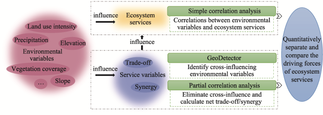
Spatial and temporal changes in ecosystem services (ESs) are driven by two types of factors: environmental factors and trade-offs/synergies between services. In the ecological conservation red line (ECRL) area, in which national ecological security and social sustainable development are guaranteed, it is particularly important to clarify the driving mechanism of ESs for the management of ecosystems. In this study, soil conservation, water yield, and carbon sequestration in Beijing’s ECRL area are quantified, and GeoDetector is used to identify the factors influencing the trade-offs/synergies between ESs. Moreover, partial correlation analysis is used to calculate the net trade-offs/synergies and compare them with the extent to which environmental variables contribute to ESs. The results are as follows: environmental variables and trade-offs/synergies have different effects on the changes in ESs, and their interactions can enhance the determinative power of the corresponding individual variable. The land use intensity is an extremely important factor affecting the trade-offs/synergies between the three services, indicating that rational land use planning in Beijing’s ECRL area is crucial for avoiding the negative impacts of trade-offs and enabling coordinated optimization of ESs. After the elimination of the cross-influence of environmental variables, the trade-offs/synergies change significantly, and the impact of environmental variables on ESs is compared with the net trade-offs/synergies. Environmental variables are the driving forces of the spatiotemporal changes in soil conservation. Precipitation and carbon sequestration have similar effects on water yield. Spatiotemporal changes in carbon sequestration are closely related to the other two services, with smaller influences from environmental variables.
ZUO Liyuan , JIANG Yuan , GAO Jiangbo , DU Fujun , ZHANG Yibo . Separating the effects of two dimensions on ecosystem services: Environmental variables and net trade-offs[J]. Journal of Geographical Sciences, 2023 , 33(4) : 845 -862 . DOI: 10.1007/s11442-023-2109-7
Figure 1 Framework for quantitative separation of ES drivers |
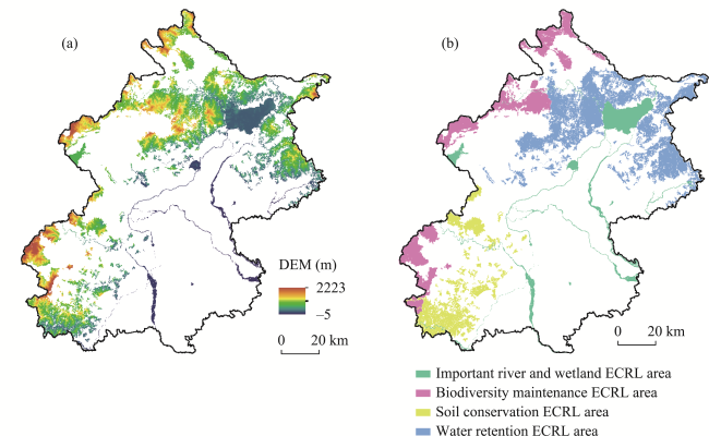
Figure 2 Elevation (a) and sub-regions (b) of the study area (Beijing) |
Table 1 Models used to quantify ESs |
| ESs | Models | Calculation method |
|---|---|---|
| Soil conservation | RUSLE model | $A=R\times K\times LS\times \left( 1-C\times P \right)$ (1) where A denotes soil conservation (t·ha−1·a−1), and R is the rainfall erosion factor. Owing to the significant seasonal differences in the precipitation in the study area, the monthly R factor is calculated and then integrated to the annual scale (Arnoldus et al., 1980). K is the soil erodibility factor, which is calculated based on the soil property data using the erosion productivity impact calculator (EPIC) (Williams et al., 1989). LS is the slope length and steepness factor. High-resolution DEM (9 m) data were used to calculate the LS to fully characterize the complexity of the elevation in the study area (Naipal et al., 2015). C is the cover and management factor, which is calculated based on the NDVI data (Cai et al., 2000). P is the practice factor, which is assigned according to the type of land use with reference to previous research on the North China Plain (Xu et al., 2012). LS, C, and P are dimensionless. |
| Water yield | InVEST model | $Y(x)=\left( 1-\frac{AET(x)}{P(x)} \right)\times P(x)$ (2) where Y(x), AET(x), and P(x) are the annual WY, annual actual evapotranspiration, and annual precipitation in grid unit x, respectively. |
| Carbon sequestration | CASA model | $NP{{P}_{t}}=APA{{R}_{t}}\times {{\varepsilon }_{t}}$ (3) where t is the period over which the NPP accumulated; and APARt and εt are the photosynthetically active radiation (MJ·m−2) and the actual light-use efficiency (gC·MJ−1) absorbed by the vegetation in pixel x in time t, respectively. |
Table 2 Types of interactions between pairs of variables |
| Description | Interaction |
|---|---|
| q(X1∩X2) < Min[q(X1), q(X2)] | Nonlinear weakening |
| Min[q(X1), q(X2)] < q(X1∩X2) < Max[q(X1), q(X2)] | Single factor nonlinear weakening |
| q(X1∩X2) > Max[q(X1), q(X2)] | Double factor |
| q(X1∩X2) = q(X1) + q(X2) | Independent |
| q(X1∩X2) > q(X1) + q(X2) | Nonlinear enhancement |
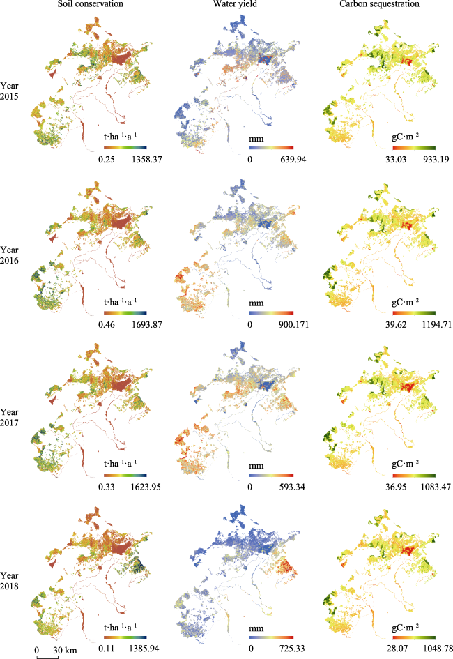
Figure 3 Spatial distribution of ESs in Beijing’s ECRL areas from 2015 to 2018 |
Table S1 Statistics of the mean value of ESs in Beijing’s ECRL areas |
| ESs | Year | Beijing’s ECRL area | Water retention ECRL area | Soil conservation ECRL area | Biodiversity maintenance ECRL area | Important river and wetland ECRL area |
|---|---|---|---|---|---|---|
| Soil conservation (t·ha‒1·a‒1) | 2015 | 345.27 | 379.34 | 510.74 | 357.53 | 42.74 |
| 2016 | 542.72 | 487.59 | 878.95 | 713.40 | 50.46 | |
| 2017 | 438.77 | 411.77 | 677.98 | 566.56 | 43.49 | |
| 2018 | 298.54 | 351.53 | 394.99 | 302.66 | 32.68 | |
| Water yield (mm) | 2015 | 131.92 | 157.08 | 153.93 | 75.57 | 124.24 |
| 2016 | 330.21 | 330.62 | 423.48 | 336.18 | 212.62 | |
| 2017 | 246.92 | 256.64 | 311.55 | 250.39 | 138.20 | |
| 2018 | 143.28 | 184.97 | 135.16 | 89.99 | 114.69 | |
| Carbon sequestration (gC·m‒2) | 2015 | 452.95 | 479.10 | 392.44 | 513.27 | 349.34 |
| 2016 | 516.91 | 532.89 | 451.76 | 618.76 | 379.72 | |
| 2017 | 480.61 | 498.50 | 436.29 | 580.33 | 316.44 | |
| 2018 | 419.44 | 445.56 | 374.40 | 493.48 | 275.07 |
Table 3 The q values of the variables influencing ESs |
| Environmental variables | Services variables | |||||||
|---|---|---|---|---|---|---|---|---|
| Elevation | Vegetation coverage | Land use intensity | Precipitation | Slope | Soil conservation | Water yield | Carbon sequestration | |
| Soil conservation | 0.233 | 0.074 | 0.133 | 0.116 | 0.530 | —— | 0.115 | 0.116 |
| Water yield | 0.062 | 0.194 | 0.443 | 0.283 | 0.099 | 0.139 | —— | 0.173 |
| Carbon sequestration | 0.318 | 0.424 | 0.289 | 0.053 | 0.192 | 0.149 | 0.224 | —— |
Note: The level of significance (p value) is <0.01. |
Table 4 Interaction between ecosystem services and environmental variables |
| Dependent variable | Water yield | Dependent variable | Soil conservation | Dependent variable | Carbon sequestration | |||
|---|---|---|---|---|---|---|---|---|
| Independent variable | Soil conservation | Carbon sequestration | Independent variable | Water yield | Carbon sequestration | Independent variable | Water yield | Soil conservation |
| Elevation | 0.172 | 0.217 | Elevation | 0.318 | 0.267 | Elevation | 0.466 | 0.363 |
| Vegetation coverage | 0.273 | 0.233 | Vegetation coverage | 0.164 | 0.145 | Vegetation coverage | 0.441 | 0.464 |
| Land use intensity | 0.502 | 0.485 | Land use intensity | 0.22 | 0.194 | Land use intensity | 0.332 | 0.335 |
| Precipitation | 0.353 | 0.459* | Precipitation | 0.206 | 0.242* | Precipitation | 0.306* | 0.232* |
| Slope | 0.165 | 0.218 | Slope | 0.579 | 0.566 | Slope | 0.309 | 0.233 |
Note: * denote that the two-factor interaction is nonlinear enhancement, and the others denote that the interaction is bivariate enhancement. |
Table 5 Correlation coefficients between ESs and the proportion of the trade-off/synergy |
| Paired ESs | Excluded factors | Correlation coefficients | Trade-off area percentage (%) | Synergy area percentage (%) |
|---|---|---|---|---|
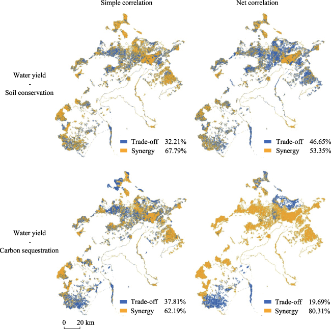
| Water yield- Soil conservation | — | 0.319 | 32.21 | 67.79 |
| Precipitation | 0.070 | 46.26 | 53.74 | |
| Land use intensity | 0.545 | 16.94 | 83.06 | |
| Precipitation and land use intensity | 0.080 | 46.65 | 53.35 | |
| Water yield- Carbon sequestration | — | 0.189 | 37.81 | 62.19 |
| Vegetation coverage | 0.286 | 32.26 | 67.74 | |
| Land use intensity | 0.381 | 25.02 | 74.98 | |
| Vegetation coverage and land use intensity | 0.528 | 19.69 | 80.31 | |
| Soil conservation- Carbon sequestration | — | 0.246 | 37.06 | 62.94 |
| Elevation | 0.379 | 24.37 | 75.63 | |
| Slope | 0.369 | 25.15 | 74.85 | |
| Land use intensity | 0.413 | 21.68 | 78.32 |
Note: The level of significance (p value) is <0.05. |
Figure 4 Spatial distribution of the tradeoff and synergy under simple and net correlations in Beijing |
Table 6 Mean values of the correlation coefficients between ESs and impact variables |
| Environmental variables | Service variables (net correlation) | |||||||
|---|---|---|---|---|---|---|---|---|
| Elevation | Vegetation coverage | Land use intensity | Precipitation | Slope | Soil conservation | Water yield | Carbon sequestration | |
| Soil conservation | 0.257 | 0.006 | 0.095 | 0.435 | 0.436 | — | 0.080 | 0.413* |
| Water yield | 0.014 | 0.048 | 0.129 | 0.599 | 0.090 | 0.080 | — | 0.528 |
| Carbon sequestration | 0.269 | 0.361 | 0.074 | 0.245 | 0.130 | 0.413* | 0.528 | — |
Note: The level of significance (p value) is <0.05. Since the elevation and slope did not change with time, only the first-order partial correlation between soil conservation and carbon sequestration was calculated, and * denotes the first-order partial correlation coefficient after excluding the land use intensity. |
| [1] |
|
| [2] |
|
| [3] |
|
| [4] |
|
| [5] |
|
| [6] |
|
| [7] |
|
| [8] |
|
| [9] |
|
| [10] |
China Council for International Cooperation on Environment and Development, Institutional Innovation of Eco-Environmental Redlining (CCICED), 2014. http://english.mee.gov.cn/Events/Special_Topics/AGM_1/AGM2014/download/201605/P020160524201838208313.pdf.
|
| [11] |
Chinese Ministry of Environmental Protection (CMEP), 2015. Technical Guidelines for the Delimitation of Ecological Conservation Redlines. Beijing, China. https://www.mee.gov.cn/gkml/hbb/bgt/201707/t20170728_418679.htm in Chinese)
|
| [12] |
|
| [13] |
|
| [14] |
|
| [15] |
|
| [16] |
|
| [17] |
|
| [18] |
|
| [19] |
|
| [20] |
|
| [21] |
|
| [22] |
|
| [23] |
|
| [24] |
|
| [25] |
|
| [26] |
|
| [27] |
|
| [28] |
|
| [29] |
Millennium Ecosystem Assessment (MEA), 2005. Ecosystems and Human Well-Being:Synthesis. Washington, DC: Island Press.
|
| [30] |
|
| [31] |
|
| [32] |
|
| [33] |
|
| [34] |
|
| [35] |
|
| [36] |
|
| [37] |
|
| [38] |
|
| [39] |
|
| [40] |
|
| [41] |
State Council of China (SCC), 2018. Beijing’s Ecological Protection Redlines. Beijing, China. http://www.gov.cn/xinwen/2018-07/13/content_5306150.htm. in Chinese)
|
| [42] |
|
| [43] |
|
| [44] |
|
| [45] |
|
| [46] |
|
| [47] |
|
| [48] |
|
| [49] |
|
| [50] |
|
| [51] |
|
| [52] |
|
| [53] |
|
| [54] |
|
| [55] |
|
| [56] |
|
| [57] |
|
| [58] |
|
| [59] |
|
| [60] |
|
| [61] |
|
/
| 〈 |
|
〉 |