Research Articles

Ecological risk assessment and ecological security pattern optimization in the middle reaches of the Yellow River based on ERI+MCR model

  • YANG Lian’an , 1, 2, 3 ,
  • LI Yali 1, 2, 3 ,
  • JIA Lujing 1, 2, 3 ,
  • JI Yongfan 1, 2, 3 ,
  • HU Guigui 1, 2, 3
Expand
  • 1. Shaanxi Key Laboratory of Earth Surface System and Environmental Carrying Capacity, Northwest University, Xi’an 710127, China
  • 2. Yellow River Institute of Shaanxi Province, Northwest University, Xi’an 710127, China
  • 3. College of Urban and Environmental Sciences, Northwest University, Xi’an 710127, China

Yang Lian’an, PhD and Associate Professor, specialized in landscape ecology and agricultural GIS. E-mail:

Received date: 2022-01-03

  Accepted date: 2022-08-25

  Online published: 2023-05-11

Supported by

National Natural Science Foundation of China(41601290)

Abstract

The middle reaches of the Yellow River represent an important area for the protection and development of the Yellow River Basin. Most of the area of the river basin is within the Loess Plateau, which establishes it as a fragile ecological environment. Firstly, using high-resolution data of land use in the watershed from the past 30 years, landscape ecological risk (LER) sample units are defined and an ecological risk index (ERI) model is constructed. Kriging interpolation is used to display the LER spatial patterns, and the temporal and spatial evolution of risk is examined. Secondly, the spatial evolution of land use landscape change (LULC) is analyzed, and the correlation between land use landscape and ecological risk is discussed. Finally, Based on the LER model, a risk-based minimum cumulative resistance (MCR) model is established, and a comprehensive protection and management network system for the ecological source-corridor-node system designed. The results suggest that in the past 30 years, LER has a high spatial correlation and areas with extremely high ecological risks are concentrated in northwest and southeast areas of the region, of which the northwest area accounts for the highest proportion. Risk intensity is closely related to the spatial pattern of land use landscape. ERI values of forestland, grasslands, and unused land and farmland are low, medium, and high, respectively. The trend of risk evolution is “overall improvement and partial deterioration”. Man-made construction and exploitation is the most direct reason for the increase of local ecological risks. The high ecological-risk areas in the northwest are dominated by deserts which reduce excessive interference by human activities on the natural landscape. Recommendations are: high-quality farmland should be protected; forestland should be restored and rebuilt; repair and adjust the existing ecosystem to assist in landscape regeneration and reconstruction; utilize the overall planning vision of “mountain, water, forest, field, lake, grass, sand” to design a management project at the basin scale; adhere to problem-oriented and precise policy implementation.

Cite this article

YANG Lian’an , LI Yali , JIA Lujing , JI Yongfan , HU Guigui . Ecological risk assessment and ecological security pattern optimization in the middle reaches of the Yellow River based on ERI+MCR model[J]. Journal of Geographical Sciences, 2023 , 33(4) : 823 -844 . DOI: 10.1007/s11442-023-2108-8

1 Introduction

Land use landscape change (LULC) is the result of a direct response of human beings to the natural ecosystem (Li et al., 2019b; Darvishi et al., 2020; Zhou et al., 2020; Assaf et al., 2021) and can have a profound impact on environmental quality (Almenar et al., 2019; Sun et al., 2020), can threaten the survival of organisms (Duveiller et al., 2020), can cause many ecological problems and affect the value of ecosystem services (Wu et al., 2020). Complex natural processes and human activities can greatly interfere with the structure and function of landscapes, and ultimately have certain adverse effects on the structure and service functions of ecosystems (Wang et al., 2021b).
Landscape Ecological Risk (LER) is used to evaluate such adverse consequences (Peng et al., 2015; Liu et al., 2018a; Luo et al., 2018; Li et al., 2019a; Wang et al., 2020a). Ecological risk assessment is an integrated system of human and environmental management (Johns et al., 2017; Carriger and Parker, 2021; Mitchell et al., 2021). Evaluating ecological risks based on changes in land-use landscapes is an important means to demonstrate LER and the spatial differentiation of LER (Jin et al., 2019). At present, research on LER mainly focuses on small river basins (e.g., Wang et al., 2017; Liu et al., 2018a; Kang et al., 2020), county areas (Liu et al., 2018a), and urban scales (Chen et al., 2021; Lin et al., 2021). Conclusions are often expressed as LER spatial agglomeration effects, regional differentiation patterns, spatio-temporal evolution characteristics and correlations between risk and land-use properties. Larger regional scales lack more systematic and complete ecological statistics and monitoring data, and there are relatively few large-scale studies (Liu et al., 2015). Many studies choose landscape patterns to establish an index system, and finally establish model algorithms. This paper builds on the results of existing research (Lv et al., 2018; Kang et al., 2020; Li et al., 2020b). We extract a landscape index, use different weights to distinguish different landscape ecological effects, and calculate ERI values with the sample as the statistical unit. This constitutes a complete LER evaluation system.
The ecological security pattern originates from the landscape spatial pattern-ecological process coupling theory (Yu et al., 2009), based on the identification, restoration and reconstruction of elements such as nodes and corridors that play an important role in the structure and function of regional ecosystems, to achieve effective ecological processes. Regulation to ensure the sustainable supply of regional ecosystem services, thereby enhancing human well-being (Peng et al., 2018; Sun et al., 2021). Ecological risk assessment can determine the spatial distribution of ecological problems, and the construction of ecological security patterns can determine the spatial distribution of ecological security. The assessment of ecological risk and ecological security together can be regarded as a complete ecological evaluation system (such as the combination of LER and MCR models), which can be used to display the ecological spatial pattern of the landscape in a study area, and finally be used to propose ecological optimization plans. The process of ecological security pattern construction requires the extraction of ecological security factors. Ecological corridors are the best and possibly only viable paths for maintaining biodiversity, migrating species and tracking climate change (Gregory et al., 2021). Ecological source areas are key to ensure the structural integrity of ecosystems (Li et al., 2020a). Ecological source areas generally refer to areas with high ecological and environmental quality and high ecological stability. Generally, areas with relatively stable ecological service functions, including forestland, rivers, lakes and scenic spots, can be selected as source areas.
Ecological sources are an important foundation for building a regional ecological network, which can provide a variety of high-quality ecosystem services, maintain a high degree of ecosystem stability, and have relatively complete ecological service functions. The process of identifying the spatial differentiation of regional landscape ecological environmental risks is similar to the comprehensive identification of ecological sources. The areas marked as having extremely low landscape ecological risks are those with the highest quality of landscape ecological environment in the basin and those with the same ecological significance as ecological source areas. Therefore, based on the principle of using ecological risk to identify ecological source areas, a risk-based minimum cumulative resistance model (MCR) model was constructed. In order to further strengthen low-risk protection, ecological security pattern identification and optimization of high-risk resistance for 2018 is performed. Through the identification and combination of regional ecological sources and ecological corridors, a spatially closely connected network system is formed (Wang et al., 2021a).
The middle reaches of the Yellow River (MYRB) have become a key management area for the protection and development of the basin, and its ecological value is extremely important. Its ecological sensitivity has been greatly affected by climate change and human activities (Xu, 2015). As population growth and urbanization accelerate, development has created important bottlenecks in the MYRB (Li et al., 2021a). The government has actively adopted ecological restoration policies such as the Three North Shelterbelt Project, the Natural Forest Protection Project, and by returning farmland to forest to affect the direction and intensity of regional land use changes (Qu et al., 2020; Tian et al., 2020).
Within the MYRB, there are regional differences between human disturbance and natural processes, leading to inconsistent spatial distribution of ecological risks (Zhang et al., 2019). Ecological protection in the MYRB needs to identify different goals and tasks for high-quality development based on internal differences, and implement precise policies according to local conditions, e.g.; highlight the management and control of “human” production and life behavior and the optimization of “land” spatial allocation; identify ecological risk areas using monitoring, and based on governance and decision-making needs. Therefore, this paper analyzes the characteristics of LULC, evaluates the impact of land use and landscape pattern changes on ecology, and finally reveals the spatial distribution patterns of LER and their spatio-temporal evolution. It is hoped the results will help guide the prevention and management of ecological risks, and promote ecological protection and high-quality development of the Yellow River Basin.

2 Methodology

2.1 Study area

The MYRB extends from Hekou Town, Togtoh County, Inner Mongolia Autonomous Region, to Taohuayu, Zhengzhou, Henan province (Figure 1). There are 13 third-level river basin areas, including Shaanxi, Shanxi, Gansu, Henan province, Inner Mongolia autonomous region and Ningxia Hui autonomous region. The area is located between 33°24'N-40°30'N and 104°12'E-113°24'E. The MYRB area is about 34.4×10⁴ km2. It accounts for 45.7% of the Yellow River Basin total area. The highest altitude is 3913 m and the lowest is 75 m. Climate types include temperate continental, temperate semi-arid and temperate semi-humid. The highest average annual precipitation is 1129 mm, and the lowest is 318 mm (Figure 1).
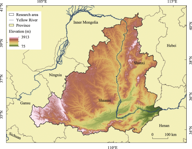
Figure 1 Location of the middle reaches of the Yellow River (MYRB)
Geomorphic features are bounded by the Great Wall, and the Mu Us desert wind-sand plateau to the north. Some 61% of the MYRB area is Loess Plateau, with loose soil, terrain fragmentation and low vegetation coverage. Therefore, heavy rainfall produces strong soil erosion, resulting in floods in the middle reaches carrying a large amount of sediment. The MYRB is the main rainstorm area in the Yellow River basin and the main source area of floods in the lower Yellow River.

2.2 Data sources

Land use data, China ecological function reserve boundary data and Normalized Difference Vegetation Index (NDVI) data was obtained from the Resource and Environment Science and Data Center (http://www.resdc.cn/Default.aspx). Land use landscape data for the MYRB is presented in Figure 2. Data on roads, residential areas, natural reserves and water resource areas were all sourced from the OpenStreetMap website (https://www.openstreetmap.org/). Digital Elevation Model (DEM) data were sourced from the geospatial data cloud site (http://www.gscloud.cn/). The years 1990, 2000, 2010 and 2018 were selected as the research time periods, representing a time scale of nearly 30 years.
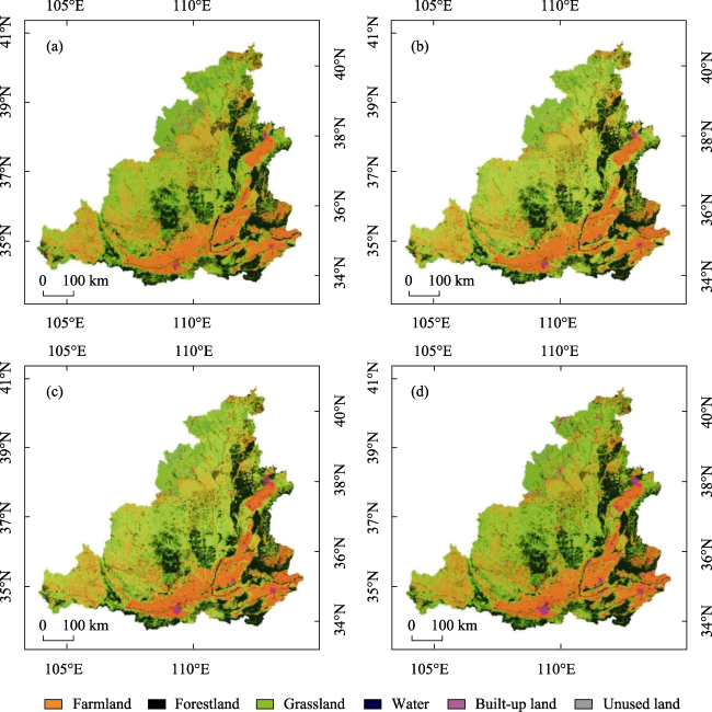
Figure 2 Land-use maps in the middle reaches of the Yellow River in 1990 (a), 2000 (b), 2010 (c) and 2018 (d)

2.3 Research methods

2.3.1 Landscape ecological pattern index

The calculation method for landscape ecological risk index is listed in Table 1.
Table 1 Landscape ecological risk index calculation method
Landscape index Formula Descriptions
Landscape
fragmentation index
${{C}_{i}}={{n}_{i}}/{{A}_{i}}$ Ni is the patches number of landscape class i; Ai is the landscape area. The index represents the process in which the landscape type tends to be complex and discontinuous patches from a single continuous whole, reflecting the degree of fragmentation (Li et al., 2020).The higher the value, the lower the stability of the corresponding landscape ecosystem.
Landscape
splitting index
${{N}_{i}}=\frac{1}{2}\sqrt{\frac{{{n}_{i}}}{A}}\times A/{{A}_{i}}$ A is the total area of all the land class. The index represents the split between different patch individuals in the landscape. The higher the value, the more complex the landscape distribution, the lower the ecological landscape stability, and the higher the ecological risk (Zhang et al., 2016).
Landscape fractal dimension index ${{F}_{i}}=\frac{2\text{ln}({{P}_{i}}/4)}{\ln {{A}_{i}}}$ Pi is the perimeter of landscape class i. The expression describing morphological changes that landscape after being disturbed by risk sources can reflect the human activities impact on the landscape (Pang, 2016). The value range is between 1 and 2, the smaller the value is, the simpler the patch shape is. The larger the value, the more complex the plaque geometry.
Landscape
disturbance
index
${{E}_{i}}=a{{C}_{i}}+b{{N}_{i}}+c{{F}_{i}}$ a=0.5, b=0.3, c=0.2 (Zhao et al., 2019). Quantifying the loss intensity of landscape subjected to external disturbance, the greater the value, the higher the ecological risk (Lin et al., 2019).
Landscape
fragility index
${{V}_{i}}$ Land use fragility: unused land = 6, water = 5, farmland = 4, grassland = 3, forestland = 2, built-up land = 1. After normalization, the index is obtained. The index indicates the ability of different landscape types to resist external disturbances. The smaller the ability to resist external disturbance, the greater the fragility and the higher the ecological risk (Fu et al., 2019).
Landscape
loss index
${{R}_{i}}={{E}_{i}}\times {{V}_{i}}$ The index refers to the difference in the ecological loss of each landscape type when it is disturbed, and it is a combination of the disturbance degree and the vulnerability index (Ye et al., 2020).

2.3.2 Landscape ecological risk index (ERI)

$ER{{I}_{k}}=\underset{i=1}{\overset{N}{\mathop \sum }}\,\frac{{{A}_{ki}}}{{{A}_{k}}}\times {{R}_{i}}$
where Aki is the area of land class i in landscape ecological risk assessment unit k, and Ak is the total area of all land class in landscape ecological risk assessment unit k. Landscape ERI was constructed according to the land use area and landscape loss index Ri. The index is used to describe the comprehensive ecological environment loss extent of the risk sample unit (Liu et al., 2018b; Jin et al., 2019). The sampling principle used was that the landscape sample area was 2-5 times as large as the average patch area, which better reflects the landscape pattern information (Wang et al., 2020b). The ArcGIS10.6 fishing net sampling tool was used, and a 2 km×2 km ecological risk assessment unit was established to construct the landscape risk index model.

2.3.3 Land use landscape change index

Single land use dynamic degree refers to the magnitude and a certain land use landscape type speed in a certain period of time (Zhang and Zang, 2019). Contrasting different periods dynamic can reflect the characteristics and intensity of land use change. The single land use landscape dynamic index is shown in formula (2). Where, LUa and LUb respectively refer to a certain land use area at the beginning and end of the research period; T is the length of the study period in years.
$K=\frac{L{{U}_{b}}-L{{U}_{a}}}{L{{U}_{a}}}\times \frac{1}{T}\times 100\text{ }\!\!%\!\!\text{ }$
The comprehensive land use dynamic degree index expresses the total change rate of all land classes in the study area (Zhang and Zang, 2019), as shown in Formula (3). Where, LUa refers to the number of land type at the beginning of the study period; ΔLUa-b refers to the absolute number of land types converted from a-th to non-a-type land during the study period; T is the length of the study period in years.
$LC=\underset{a=1}{\overset{n}{\mathop \sum }}\,\text{ }\!\!\Delta\!\!\text{ }L{{U}_{a-b}}/2\underset{a=1}{\overset{n}{\mathop \sum }}\,L{{U}_{a}}\times \frac{1}{T}\times 100\text{ }\!\!%\!\!\text{ }$
Mean center and standard deviational ellipse (SDE): Directional distribution analysis is used to demonstrate the variation and dynamic change process of land use (Gao et al., 2018). The area-weighted mean center is the center position of each land use landscape class within the study area, which represents the spatio-temporal pattern of land use. The SDE is created to analyze the spatial characteristics of land class and express its tendency of concentration, dispersion and direction.

2.3.4 Spatial correlation

The global Moran’s I describes whether there is a significant spatial correlation between the attribute values of elements and the adjacent attribute values (Gong et al., 2019; Ye et al., 2020). Its value is between -1 and 1. When Moran’s I is greater than 0, it indicates positive correlation and convergent agglomeration. The local spatial autocorrelation index uses Anselin Local Moran’s I (Lisa) to detect the aggregation area. Through correlation between the same attribute value of the regional sample unit and the adjacent unit to show the local agglomeration and dispersion effects (Ye et al., 2020).

2.3.5 MCR and gravity model

$MCR={{f}_{min}}\left( \underset{j=n}{\overset{i=m}{\mathop \sum }}\,{{D}_{ij}}\times {{R}_{i}} \right)$
where MCR is the minimum cumulative resistance value, fmin is the function of the product between MCR and variable (Dij×Ri), Dij is the distance from the source j to the target source i, Ri is the diffusion resistance coefficient of the landscape unit in a certain direction in space (Huang et al., 2019).
${{G}_{ab}}=\frac{{{N}_{a}}-{{N}_{b}}}{D_{ab}^{2}}=\frac{L_{max}^{2}\text{ln}({{S}_{a}}{{S}_{b}})}{L_{ab}^{2}{{P}_{a}}{{P}_{b}}}$
where Gab is the interaction intensity between patch a and patch b; Na and Nb represent the corresponding weight values of sources a and b, respectively. Dab is the standard value of corridor resistance between source areas (Nie et al., 2021); Lmax is the maximum resistance of all corridors in the study area; Sa and Sb are the areas of patch a and patch b; Lab is the cumulative resistance value of the corridor between patch a and patch b; Pa and Pb are the resistance values of patch a and patch b (Zhang et al., 2021).

3 Results

3.1 Landscape ecological risk assessment and spatial evolution analysis

3.1.1 LER spatial distribution and autocorrelation analysis

Based on the ERI natural breaks value of 4 years as a reference, try to maximize the difference between each level (Kang et al., 2020; Chen et al., 2021), and finally set it to less than 0.0343 (extremely low), 0.0343-0.0420 (low), 0.0420-0.0480 (medium), 0.0480-0.0554 (high), greater than 0.0554 (extremely high). The LER results (Figure 3) show that extremely high-risk areas were concentrated in the northwest and southeast of the MYRB, and their regional distribution shows a shrinking trend over time. Large high-risk areas in the northern and central regions reduced to medium-risk areas over the sampled period. Extremely low-risk areas were distributed in the central, eastern and southern mountainous areas. These areas show sporadic growth, with the most significant growth in the northern and central regions. The proportion of medium-risk areas increased from 24.86% in 1990 to 33.58% in 2018. The proportion of extremely high and high LER regions decreased from 5.40% to 3.91%. The proportion of high-risk areas dropped from 45.08% to 34.08%.
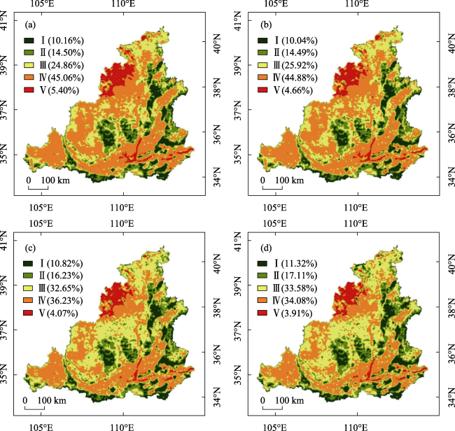
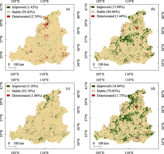
Figure 3 Maps of the landscape ecological risk (LER) in the middle reaches of the Yellow River for 1990 (a), 2000 (b), 2010 (c), and 2018 (d) (Note: I: Extremely low, II: Low, III: Medium, IV: High, V: Extremely high. The number in parentheses is the area percentage of each LER class.)
The Moran’s I of the global spatial correlations in 1990, 2000, 2010, and 2018 were 0.738611, 0.724356, 0.715859, 0.710663. LER presents a spatial agglomeration effect over the entire region. Areas with high LER values have high values in adjacent areas, and areas with low LER values have low values in adjacent areas. The local spatial autocorrelation results (Figure 4) suggest that the “high-high (HH)” agglomeration area and the extremely high landscape ecological risk area had almost the same spatial distributions and were located in the northwest and southeast. The “high” agglomeration area in the southeast spreads to the urban construction area.
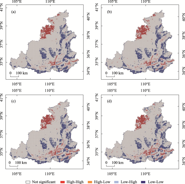
Figure 4 Local spatial autocorrelation (Lisa) of the landscape ecological risk in the middle reaches of the Yellow River for 1990 (a), 2000 (b), 2010 (c), and 2018 (d)

3.1.2 The temporal evolution of the spatial pattern of LER

As Figure 5 shows, from 1990 to 2000, LER increased significantly, and the ecological environment deteriorated more than recovered. From 2000 to 2010, the proportion of ecological restoration was large, reaching 13%. From 2010 to 2018, the risk in the northwest decreased. In short, over the past 30 years (Figure 5d), there has been a significant decrease in LER, the overall landscape ecology has been improved, and local risks have decreased.
Figure 5 Landscape ecological risk change spatial distribution in the middle reaches of the Yellow River for 1990 to 2000 (a), 2000 to 2010 (b), 2010 to 2018 (c), and 1990 to 2018 (d) (The number in the parentheses is the percentage of area for each LER change class.)
The typical LER-increase areas of Zones I, II, and III can be used to observe the relationship between the changes of land use types (Figure 6). Grassland areas in Zone I decreased, while woodland, built-up land and unused land increased. Built-up land, grassland and farmland in Zone II increased, and large areas of forestland were regularly converted into grassland and farmland. The surrounding built-up land grew in patches, with obvious traces of artificial transformation. Farmland and built-up land in Zone III increased significantly, occupying forestland and grassland resources. Vegetation in areas of increased risk clearly degraded. To summarize, spatial patterns of the temporal evolution of ecological risk are significant, and there is a correlation between the transition of ecological risk level and the transfer of land use type, which needs to be further explored.
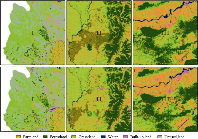
Figure 6 Changes in I, II, III internal land use landscapes in the middle reaches of the Yellow River

3.2 Correlation between LULC and LER

3.2.1 Land use landscape spatial pattern evolution analysis

Farmland is concentrated in the south and southeast plain area. The landscape patches are in the northeast-southwest direction. The average center is located in the central area, which slightly shifted to the northwest after 2000, and there are no obvious changes in the standard deviational ellipse (SDE). Forestland is mainly distributed in the central, eastern, and southern mountainous areas, and the SDE orientation is “northeast-southwest”. Grassland is the most widely distributed, second only to farmland, and for this land-use type the SDE orientation is “northeast-southwest” and the mean center is located in the northwest. The center of gravity did not change significantly. Patches of land-use associated with water resources were orientated in the “north-south” direction, and with the center moving to the southeast. Built-up land is mainly distributed in urban areas with rapid economic development. The SDE direction for built-up land is “northeast-southwest” and the mean center is located in the central region and experienced a large shift to the north after 2000. Unused land is concentrated in the Mu Us Sandy Land in the northwest. For unused land the SDE shows a “northeast-southwest” direction, and the ellipse showed a shrinking trend. The mean center is located in the northwest and moves southwest (Figure 7).
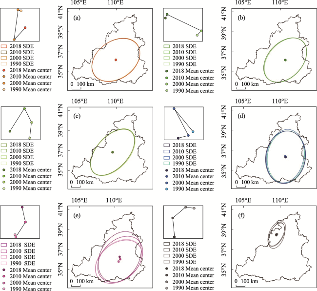
Figure 7 Map of land use landscape center of gravity transfer in the middle reaches of the Yellow River (a. farmland, b. forestland, c. grassland, d. water, e. built-up land, f. unused land)
Tables 2 and 3 are obtained by calculating the land use change index. The MYRB land-use landscape structure is farmland > grassland > forestland > built-up land > unused land > water. Over the study period, the proportion of farmland first increased and then decreased with the year 2000 as the turning point. Forests and grasslands showed a clear growth trend. The area of built-up land increased from 2.21% in 1990 to 4.47% in 2018, and then continued to increase. The proportion of unused land continuously declined as it was converted into forestland, farmland and grassland. 10.47% of unused land was converted into grassland. Some of the unused land was transferred to farmland and built-up land. The comprehensive dynamic degree of land use was 0.08%, 0.34% and 0.53% during each time period, indicating that the overall land-use pattern has changed strongly over the past 30 years, and the degree of use has been continuously improved. After 2000, the rate of land-use pattern change has increased significantly, while the stability of land-use landscape pattern has declined.
Table 2 Landscape area (CA, ha) and dynamic attitude towards change (K, %)
Landscape type CA1990 CA2000 CA2010 CA2018 K1990-2000 K2000-2010 K2010-2018
Farmland 13,782,030.00 13 801,271.76 13 017,665.97 12,768,659.91 0.01% -0.57% -0.24%
Forestland 6,696,526.00 6 686,714.07 6 915,599.91 6,895,743.93 -0.01% 0.34% -0.04%
Grassland 11,809,910.00 11 854,688.40 12 061,886.94 12,032,993.97 0.04% 0.17% -0.03%
Water 387,730.20 365,374.26 356,842.44 359,651.79 -0.58% -0.23% 0.10%
Farmland 758,543.20 846,784.35 1 241,309.34 1 534,453.02 1.16% 4.66% 2.95%
Unused land 936,875.30 816,729.57 778,366.08 772,511.13 -1.28% -0.47% -0.09%
Table 3 Land use landscape transfer matrix (ha)
1990 2018
Farmland Forestland Grassland Water Built-up land Unused land
Farmland 11,207,331.31 172,954.17 1,182,919.46 70,113.81 105,260.4 29,646.18
Forestland 339,738.88 6,151,248.53 380,353.58 6169.55 4390.65 13,539.76
Grassland 1,517,517.39 318,377.66 9,959,568.41 24,525.11 17,426.69 195,166.24
Water 61,514.68 7256.91 26,310.13 257,050.99 1859.36 5646.93
Built-up land 639,541.75 40,772.37 176,650.21 16,966.44 628,571.43 31,902.79
Unused land 14,218.80 4379.22 80,871.1 11,162.46 993.94 660,868.86

3.2.2 Correlation LER and land-use landscape evolution

There are differences in the LER generated by land-use landscape types, and the differences are described below using changes in the landscape index (Table 4). The number of farmland patches is the largest, with a growth rate of 5% from 2010 to 2018, the landscape fragmentation index increased by 14.29%, the landscape disturbance index and landscape loss index increased, the stability decreased, and the ecological loss increased. The fragmentation index of forestland landscape increased, with the largest increase from 2000 to 2010. The number of grassland patches ranks second, the patch shapes are complex, and the landscape fractal dimension index is greater than 1.5, which is greatly disturbed by human activities. From 2000 to 2010, the number of built-up land patches increased by 14.7%, the fragmentation index decreased by 21.82%, the split index decreased by 26.94%, the landscape fractal dimension index increased, and the connectivity of landscape patches increased. The number of unused land parcels continued to increase, with a growth rate of 29.71% from 2010 to 2018. Taking the year 2000 as the node, the fractal dimension of unused land increases, the desert patches become fragmented, from simple to complex, and the degree of landscape connection decreases.
Table 4 Land use landscape pattern index
Land use
landscape
Year Splitting
index
Fractal dimension
index
Disturbance
index
Fragility
index
Loss
index
Farmland 1990 0.00064 1.50357 0.30091 0.19050 0.05732
2000 0.00065 1.50424 0.30104 0.19050 0.05735
2010 0.00068 1.50343 0.30089 0.19050 0.05732
2018 0.00072 1.50536 0.30129 0.19050 0.05740
Forestland 1990 0.00094 1.45330 0.29094 0.09524 0.02771
2000 0.00095 1.45419 0.29112 0.09524 0.02773
2010 0.00095 1.45698 0.29168 0.09524 0.02778
2018 0.00096 1.45772 0.29183 0.09524 0.02779
Grassland 1990 0.00060 1.51036 0.30225 0.14286 0.04318
2000 0.00060 1.51063 0.30231 0.14286 0.04319
2010 0.00057 1.50714 0.30160 0.14286 0.04309
2018 0.00059 1.50803 0.30178 0.14286 0.04311
Water 1990 0.00474 1.43508 0.28844 0.23810 0.06868
2000 0.00495 1.43915 0.28932 0.23810 0.06888
2010 0.00504 1.43523 0.28856 0.23810 0.06870
2018 0.00543 1.44353 0.29034 0.23810 0.06913
Built-up land 1990 0.00829 1.47142 0.29678 0.04762 0.01413
2000 0.00748 1.46844 0.29593 0.04762 0.01409
2010 0.00546 1.47005 0.29565 0.04762 0.01408
2018 0.00453 1.46758 0.29488 0.04762 0.01404
Unused land 1990 0.00944 1.38924 0.28068 0.28571 0.08020
2000 0.00211 1.39525 0.27968 0.28571 0.07991
2010 0.00246 1.40134 0.28101 0.28571 0.08029
2018 0.00283 1.40724 0.28230 0.28571 0.08066
The following correlation analysis is carried out from the perspective of the spatial distribution and evolution of land-use landscape and LER (Figure 8). Extremely high-risk areas are dominated by farmland, grassland and unused land. Farmland in the high-risk area constitutes about 59%, and grassland about 30%. The medium-risk areas are mainly farmland and grassland. The forestland and grassland areas dominate in low-risk areas. Extremely low-risk areas are dominated by forestland, accounting for about 80%. From 1990 to 2018, the proportion of farmland and unused land in extremely high-risk areas decreased, and forestland increased. Forestland also increased in high-risk areas. Farmland in the medium-risk areas increased, while forestland and grassland decreased. Forestland in extremely low-risk areas decreased. After 2000, built-up land in various risk areas increased significantly.
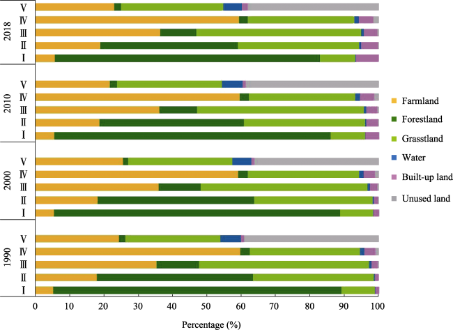
Figure 8 The proportion of land use landscape area in landscape ecological risk areas in the middle reaches of the Yellow River from 1990 to 2018

3.3 Ecological security pattern based on the landscape ecological risk

3.3.1 Ecological security factors based on the MCR Model

Following the concepts of the MCR model, extremely low and low LER areas are regarded as ecological sources, and 14 of these larger source areas are used for security pattern analysis. An ecological security assessment was performed based on the results of an ecological risk analysis for 2018. Resistance grade values were first assigned (Table 5) to each resistance factor grade, and then 4000 random sample points were applied to extract resistance factor values. Spatial principal component analysis was then used to spatially reduce the indicators and perform KMO (0.624) analysis. As a result, there are three principal components with eigenvalues greater than 1, and the comprehensive weight of each factor is calculated according to the contribution rate of the principal component and the eigenvalue (Tables 6 and 7). Finally, the resistance surface is obtained by superimposing calculations based on the weight value in ArcGIS 10.6 (Figure 9a).
Table 5 Resistance factor evaluation system and weights
Resistance factors Resistance level
Unit 1 2 3 4
Slope ° <7 7-15 15-25 >25
DEM m 800 800-1200 1200-1700 >1700
Land use Forestland
Grassland
Water Farmland Built-up land
Unused land
NDVI >65% 50%-65% 35%-50% <35%
Distance from natural reserves m <2000 2000-4000 4000-6000 >6000
Distance from water area m <500 500-1000 1000-1500 >1500
Distance from residential areas m >2000 1500-2000 1000-1500 <1000
Distance from roads m >3000 2000-3000 1000-2000 <1000
Table 6 Principal component eigenvalues and contribution rate
PC Eigen value Contribution rate (%) Cumulative contribution rate (%)
1 1.958 24.481 24.481
2 1.237 15.464 39.944
3 1.053 13.166 53.111
4 0.963 12.033 65.144
5 0.874 10.923 76.066
6 0.749 9.367 85.433
7 0.617 7.716 93.149
8 0.548 6.851 100.000
Table 7 Principal component loading matrix
PC1 PC2 PC3 Weight
Slope -0.682 -0.373 -0.110 0.275
DEM -0.608 0.077 0.507 0.044
Landcover 0.687 0.134 0.026 0.211
NDVI 0.396 0.453 0.539 0.300
Distance from natural reserves 0.138 0.271 -0.628 0.028
Distance from water area -0.380 0.638 0.047 0.043
Distance from residential areas 0.251 -0.569 0.304 0.005
Distance from roads 0.517 -0.253 0.058 0.093
Figure 9 Resistance value distribution in the middle reaches of the Yellow River (a), and spatial distribution of the minimum cumulative resistance (b)
The first principal component has a large contribution of land use and slope, the second principal component has the largest contribution of distance from water areas and residential areas, and the third principal component has a large contribution of distance from and NDVI (vegetation coverage). The resistance value in the area is calculated based on the weight value of the resistance factor. As shown in Figure 9, high resistance values have a strong spatial relationship with unused land and built-up land, which are concentrated in the northwest and in urban agglomerations, and the resistance values of areas with high vegetation coverage are obviously lower.
The cost distance can be used to obtain the minimum cumulative resistance surface (Figure 9b), and then to reveal the cost path based on the minimum cumulative resistance surface and the ecological source. An ecological corridor is a bridge connecting regional ecological sources which is conducive to ecological circulation and forms a complete interconnected ecosystem (Fu et al., 2020). A total of 91 ecological corridors have been formed. A gravity model is used to screen the ecological corridors (Table 8). There are 59 ecological corridors with importance less than 1000, 21 second-level ecological corridors with importance between 1000 and 4000, and 11 first-level ecological corridors with importance greater than 4000. Hydrological analysis is used to determine the highest resistance value distribution line from the minimum cumulative resistance surface (Yu et al., 2022), and intersect it with the first- and second-level ecological corridors to obtain the lowest and highest values. The intersection of resistance paths indicates the first-level ecological node, with a total of 34, and 67 ecological nodes are obtained by extracting the intersection points between potential ecological corridors.
Table 8 Interaction intensity of the ecological sources
Importance intensity Ecological sources
1 2 3 4 5 6 7
Ecological sources 1 496.363 3251.784 493.007 383.939 314.764 315.858
2 1835.816 6627.223 7788.075 1007.024 2968.156
3 1271.954 1157.586 908.272 920.473
4 3011.552 609.881 1455.133
5 1741.775 17393.908
6 3146.495
7
8
9
10
11
12
13
14
Importance intensity Ecological sources
8 9 10 11 12 13 14
Ecological sources 1 135.354 139.319 261.405 202.370 549.194 10,961.767 5029.719
2 308.224 362.369 2142.793 1445.406 1830.386 912.972 492.734
3 220.694 240.434 615.857 471.708 1902.202 13,376.014 1932.548
4 605.245 755.824 3786.867 1969.244 988.864 844.004 535.114
5 320.027 372.389 3742.240 3054.440 2995.553 644.070 363.737
6 141.933 154.790 614.531 534.548 18,111.769 498.506 257.936
7 233.010 264.684 1908.673 1680.415 4604.026 510.890 284.662
8 23263.813 527.708 435.166 200.630 180.063 147.014
9 659.663 542.943 220.362 192.012 148.768
10 30,887.623 882.213 403.579 267.825
11 735.599 307.211 206.296
12 928.662 435.460
13 4278.296
14

3.3.2 Ecological security spatial distribution

Ecological source areas are an important part of the ecological security pattern, and ensuring stability is the foundation of regional ecological security. The ecological source areas of the middle reaches of the Yellow River are mainly in the east, middle and south. The eastern and central areas are mainly used for ecosystem protection and restoration, and the south is dominated by the Qinling Mountains.
The ecological corridor is the path of least resistance in the process of species migration. Human intervention leads to the destruction of ecosystems and ecological corridors and their functions in the natural landscape environment. Revitalization and maintenance of river flows are essential for the preservation and reconnection of the existing bio-corridors and to help the natural environment adapt to climate change (Agócsová et al., 2020). Key corridors are mainly distributed in the southeastern part of the study area, in the east and middle areas, where there are extremely high ecological risk values. These areas are also ones where the intensity of urban construction is enhanced, and the ecological protection and construction of corridors need to be further strengthened. Other potential corridors are mainly distributed in the central area of the study area, showing a “north-south” orientation.
Ecological nodes are generally located in areas with relatively fragile ecological functions and are prone to be destroyed. They are generally located at the weakest point of ecological function in an ecological corridor, and are mainly composed of the intersection of the smallest and the largest paths or the intersection of the smallest paths. There are many ecological nodes, which are important areas for dynamic supervision and restoration. Regional ecological risks should be reduced and regional ecological security should be ensured (Figure 10).
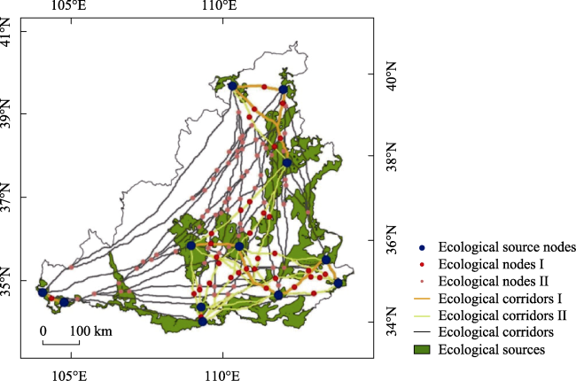
Figure 10 Spatial pattern of ecological sources, ecological corridors and ecological nodes in the middle reaches of the Yellow River

3.3.3 Ecological security pattern optimization

The results for ecological security optimization can be summarized as follows (Figure 11).
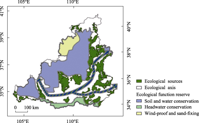
Figure 11 Ecological security optimization zoning in the middle reaches of the Yellow River
Ecological axis area: This area is an area with fragile ecological patches, strong interference from human activities, strong construction and development intensity, and economic development. The area is a key control area and a buffer area to ensure that the boundary of the ecological source is not disturbed. The protection and management of ecological corridors are very important in this area. The ecological function of rivers should be guaranteed.
Soil and water conservation area: This is the Loess Plateau ecological function reserve. This area is mainly given over to water and soil conservation. Here vegetation zones should be managed and reasonable measures for ecological protection and restoration taken. It is located in the middle and west of the MYRB. It has a wide distribution area, strong ecological resistance, and few ecological sources.
Headwater conservation area: This area is mainly the ecological function protection area in the Qinling Mountains. It is an ecological protection barrier in the northwest and a key ecological source protection area. Here, ecological and environmental protection and restoration measures should be continued, and the protection and restoration of habitats for rare and endangered species strengthened. The construction of ecological corridors should be actively promoted, and the living space of wild animals and plants expanded.
Wind-proof and sand-fixing area: This is the Mu Us Sandy Land ecological function reserve. The area exhibits extremely high ecological risks. The protection and ecological restoration of Mu Us Sandy Land is the primary focus of work in this area in recent years, and the optimization of the landscape patterns here is very important.

4 Discussion

Ecological risk assessment results can be compared to the previously published research. Urban and desert landscapes are at the highest ecological risk in the Loess Plateau, with obvious spatial differences (Jing et al., 2021). The windy areas in northern Shaanxi are also at great risk (Fu et al., 2019). Vegetation change and urbanization are the main influencing factors (Fu et al., 2019). The implementation of ecological engineering has played a role in promoting the reduction of landscape ecological risks, and human intervention, especially urban expansion, has led to a significant increase in regional ecological risks (Jing et al., 2021). Experts recommend strengthening the intensive and efficient use of urban land while limiting the development of small towns within the harsh northern environments (Jing et al., 2021). The LER results presented here show that extremely high-risk areas are concentrated in the northwest and southeast of the MYRB, and high risks are mainly generated by sandy land and built-up land. Based on the ecological risk assessment of LER, this study further constructed the ecological security pattern of the river basin, which, as a complete evaluation system, can provide reference for related research work. However, landscape ecological risk assessment is only one aspect of ecological environment quality assessment. With the diversification of assessment methods and data, the function, structure and stress of the river basin ecological environment are comprehensively considered, and more diversified assessment methods and models are constructed.
In the process of constructing the ecological security pattern, grassland, forestland, and water are often directly selected as natural ecological spaces to screen ecological sources (Zhang et al., 2019), In recent years, comprehensive extraction methods of ecological sources based on habitat quality (Li et al., 2021b) and ecological sensitivity have been applied. In this paper, the ecological risk assessment process is used to comprehensively identify ecological sources, and areas with low risk are regarded as source areas. A risk-based MCR model was constructed, which is a new application in the research of ecological security. In future study, ecological security pattern research can screen ecological sources from multiple perspectives, and conduct research based on the results of comprehensive evaluation of environmental quality. At the same time, the construction of the resistance surface is an important step in ecological security assessment, and areas with high ecological risk or poor environmental quality can be considered into the resistance factor assessment process. From the perspective of research methods, the ecological security pattern can adopt new network construction methods, such as granular inversion methods and combined models such as circuit theory.

5 Conclusions

By constructing the ERI, the LER in the MYRB is obtained. The LER in the MYRB has high spatial correlation, showing a trend of “overall improvement and partial deterioration”. Construction and mining are the immediate reasons for the increase in LER in the southeast. The northwest core of the high ecological risk area is directly related to the desert ecological environment. There is a strong correlation between LER and the spatial pattern of land-use landscapes. LER levels vary with the proportion of land types within the risk area.
It is recommended to protect high-quality farmland, especially from urban expansion areas, and promote ecological agriculture to provide the dual functions of product service and ecological adjustment. Forest landscape is the key to ecological pattern optimization. The northwest LER area focuses on sand control. In the process of ecological restoration, excessive interference from human activities on the natural landscape should be avoided to prevent the rapid increase of local regional risks. Using the characteristics of LER space agglomeration, protection management plans should be formulated to assist in landscape renovation.
The combination of LER and MCR extracts ecological security factors and constitutes the ecological security pattern of the basin. With ecological restoration as the background, construct MYRB’s security pattern optimization partition. The ecological security pattern of the MYRB focuses attention on the protection of ecological source areas, ensuring soil and water conservation and ecological improvement in water source conservation areas, and continuously improving the ecological restoration of the Mu Us Sandy Land. The comprehensive protection and management of the ecological source-corridor-node system should be urgently considered. The concept of an “ecological axis” should be used as buffers to ensure ecological sources.
[1]
Agócsová Á, Högyeová M, Chodasová Z et al., 2020. River Restoration as a method towards harmonization of natural habitats in the context of ecological corridors preservation: A case study on the Hron River. IOP Conference Series: Materials Science and Engineering, 960(2): 022058.

[2]
Almenar J B, Bolowich A, Elliot T et al., 2019. Assessing habitat loss, fragmentation and ecological connectivity in Luxembourg to support spatial planning. Landscape and Urban Planning, 189: 335-351.

DOI

[3]
Assaf C, Adams C, Ferreira F F et al., 2021. Land use and cover modeling as a tool for analyzing nature conservation policies: A case study of Juréia-Itatins. Land Use Policy, 100: 104895.

DOI

[4]
Carriger J F, Parker R A, 2021. Conceptual Bayesian networks for contaminated site ecological risk assessment and remediation support. Journal of Environmental Management, 278(2): 111478.

DOI

[5]
Chen X, Xie G, Zhang J, 2021. Landscape ecological risk assessment of land use changes in the coastal area of Haikou City in the past 30 years. Acta Ecologica Sinica, 41(3): 975-986. (in Chinese)

[6]
Darvishi A, Yousefi M, Marull J, 2020. Modelling landscape ecological assessments of land use and cover change scenarios: Application to the Bojnourd Metropolitan Area (NE Iran). Land Use Policy, 99: 105098.

DOI

[7]
Duveiller G, Caporaso L, Abad-Vias R et al., 2020. Local biophysical effects of land use and land cover change: Towards an assessment tool for policy makers. Land Use Policy, 91: 104382.

DOI

[8]
Fu W, Fu B, Hu W, 2019. Landscape ecological risk assessment under the influence of typical human activities in Loess Plateau, northern Shaanxi. Journal of Ecology and Rural Environment, 35(3): 290-299. (in Chinese)

[9]
Fu Y, Shi X, He J et al., 2020. Identification and optimization strategy of county ecological security pattern: A case study in the Loess Plateau, China. Ecological Indicators, 112: 106030.

DOI

[10]
Gao J, Xie W, Han Y et al., 2018. The evolutionary trend and the coupling relation of gravity center moving of county-level population distribution, economical development and grain production during 1990-2013 in Henan province. Scientia Geographica Sinica, 38(6): 919-926. (in Chinese)

DOI

[11]
Gong J, Xie Y, Cao E et al., 2019. Integration of InVEST-habitat quality model with landscape pattern indexes to assess mountain plant biodiversity change: A case study of Bailongjiang watershed in Gansu province. Journal of Geographical Sciences, 29(7): 1193-1210.

DOI

[12]
Gregory A, Spence E, Beier P et al., 2021. Toward best management practices for ecological corridors. Land, 10(2): 140-164.

DOI

[13]
Huang M, Yue W, Feng S et al., 2019. Analysis of spatial heterogeneity of ecological security based on MCR model and ecological pattern optimization in the Yuexi county of the Dabie Mountain Area. Journal of Natural Resources, 34(4): 771-784. (in Chinese)

DOI

[14]
Jin X, Jin Y, Mao X, 2019. Ecological risk assessment of cities on the Tibetan Plateau based on land use/land cover changes: Case study of Delingha city. Ecological Indicators, 101: 185-191.

DOI

[15]
Jing P, Zhang D, Ai Z et al., 2021. Natural landscape ecological risk assessment based on the three-dimensional framework of pattern-process ecological adaptability cycle: A case in Loess Plateau. Acta Ecologica Sinica, 41(17): 7026-7036. (in Chinese)

[16]
Johns A F, Graham S E, Harris M J et al., 2017. Using the Bayesian network relative risk model risk assessment process to evaluate management alternatives for the South River and upper Shenandoah River, Virginia. Integrated Environmental Assessment and Management, 13(1): 100-114.

DOI PMID

[17]
Kang Z, Zhang Z, Wei H et al., 2020. Landscape ecological risk assessment in Manas River Basin based on land use change. Acta Ecologica Sinica, 40(18): 6472-6485. (in Chinese)

[18]
Li H, Shi C, Sun P et al., 2021a. Attribution of runoff changes in the main tributaries of the middle Yellow River, China, based on the Budyko model with a time-varying parameter. CATENA, 206: 105557.

DOI

[19]
Li Q, Zhang Z, Wan L et al., 2019a. Landscape pattern optimization in Ningjiang River Basin based on landscape ecological risk assessment. Acta Geographica Sinica, 74(7): 1420-1437. (in Chinese)

[20]
Li S, Xiao W, Zhao Y et al., 2020a. Incorporating ecological risk index in the multi-process MCRE model to optimize the ecological security pattern in a semi-arid area with intensive coal mining: A case study in northern China. Journal of Cleaner Production, 247: 119143.

DOI

[21]
Li S, Zhao Y, Xiao W et al., 2021b. Optimizing ecological security pattern in the coal resource-based city: A case study in Shuozhou city, China. Ecological Indicators, 130: 108026.

DOI

[22]
Li W, Wang Y, Xie S et al., 2020b. Impacts of landscape multifunctionality change on landscape ecological risk in a megacity, China: A case study of Beijing. Ecological Indicators, 117: 106681.

DOI

[23]
Li Y, Li Y, Fan P et al., 2019b. Land use and landscape change driven by gully land consolidation project: A case study of a typical watershed in the Loess Plateau. Journal of Geographical Sciences, 29(5): 719-729.

DOI

[24]
Lin J, Lin M, Chen W et al., 2021. Ecological risks of geological disasters and the patterns of the urban agglomeration in the Fujian Delta region. Ecological Indicators, 125: 107475. doi: 10.1016/J.ECOLIND.2021.107475.

DOI

[25]
Liu C, Zhang K, Liu J, 2018a. A long-term site study for the ecological risk migration of landscapes and its driving forces in the Sanjiang Plain from 1976 to 2013. Acta Ecologica Sinica, 38(11): 3729-3740. (in Chinese)

[26]
Liu D, Chen H, Liang X et al., 2018b. The dynamic changes to ecological risk in the loess hilly-gully region and its terrain gradient analysis: A case study of Mizhi county, Shaanxi province, China. Acta Ecologica Sinica, 38(23): 8584-8592. (in Chinese)

[27]
Liu Y, Wang Y, Peng J et al., 2015. Urban landscape ecological risk assessment based on the 3D framework of adaptive cycle. Acta Geographica Sinica, 70(7): 1052-1067. (in Chinese)

DOI

[28]
Luo F, Liu Y, Peng J et al., 2018. Assessing urban landscape ecological risk through an adaptive cycle framework. Landscape and Urban Planning, 180: 125-134.

DOI

[29]
Lv L, Zhang J, Sun C et al., 2018. Landscape ecological risk assessment of Xi River Basin based on land-use change. Acta Ecologica Sinica, 38(16): 5952-5960. (in Chinese)

[30]
Mitchell C J, Lawrence E, Chu V R et al., 2021. Integrating metapopulation dynamics into a Bayesian network relative risk model: Assessing risk of pesticides to Chinook salmon (Oncorhynchus tshawytscha) in an ecological context. Integrated Environmental Assessment and Management, 17(1): 95-109.

DOI PMID

[31]
Nie W, Shi Y, Siaw M J et al., 2021. Constructing and optimizing ecological network at county and town scale: The case of Anji county, China. Ecological Indicators, 132: 108294.

DOI

[32]
Peng J, Dang W, Liu Y et al., 2015. Review on landscape ecological risk assessment. Acta Geographica Sinica, 70(4): 664-677. (in Chinese)

DOI

[33]
Peng J, Li H, Liu Y et al., 2018. Identification and optimization of ecological security pattern in Xiong’an New Area. Acta Geographica Sinica, 73(4): 701-710. (in Chinese)

[34]
Qu S, Hu S, Li W et al., 2020. Interaction between urban land expansion and land use policy: An analysis using the DPSIR framework. Land Use Policy, 99: 104856.

DOI

[35]
Sun F, Zhang J, Wang P et al., 2021. Construction and evaluation of urban ecological security pattern: A case study of Suzhou city. Geographical Research, 40(9): 2476-2493. (in Chinese)

DOI

[36]
Sun R, Wu Z, Chen B et al., 2020. Effects of land-use change on eco-environmental quality in Hainan Island, China. Ecological Indicators, 109: 105777.

DOI

[37]
Tian J, Wang B, Zhang C et al., 2020. Mechanism of regional land use transition in underdeveloped areas of China: A case study of northeast China. Land Use Policy, 94: 104538.

DOI

[38]
Wang B, Ding M, Li S et al., 2020a. Assessment of landscape ecological risk for a cross-border basin: A case study of the Koshi River Basin, central Himalayas. Ecological Indicators, 117: 106621.

DOI

[39]
Wang H, Liu X, Zhao C et al., 2021a. Spatial-temporal pattern analysis of landscape ecological risk assessment based on land use/land cover change in Baishuijiang National Nature Reserve in Gansu province, China. Ecological Indicators, 124: 107454.

DOI

[40]
Wang J, Bai W, Tian G, 2020b. A review on ecological risk assessment of land use. Journal of Natural Resources, 35(3): 576-585. (in Chinese)

DOI

[41]
Wang S, Wu M, Hu M et al., 2021b. Promoting landscape connectivity of highly urbanized area: An ecological network approach. Ecological Indicators, 125: 107487.

DOI

[42]
Wang T, Zhang C, Yu X et al., 2017. Effect of land use change on landscape ecological security in Erhai basin. Chinese Journal of Ecology, 36(7): 2003-2009. (in Chinese)

[43]
Wu C, Chen B, Huang X et al., 2020. Effect of land-use change and optimization on the ecosystem service values of Jiangsu province, China. Ecological Indicators, 117: 106507.

DOI

[44]
Xu J, 2015. Runoff renewability in the middle Yellow River in response to human activity and climate change. Journal of Natural Resources, 30(22): 423-432. (in Chinese)

[45]
Ye S, Song C, Shen S et al., 2020. Spatial pattern of arable land-use intensity in China. Land Use Policy, 99: 104845.

DOI

[46]
Yu J, Tang B, Chen Y et al., 2022. Landscape ecological risk assessment and ecological security pattern construction in landscape resource-based city: A case study of Zhangjiajie city. Acta Ecologica Sinica, 42(4): 1290-1299. (in Chinese)

[47]
Yu K, Wang S, Li D et al., 2009. The function of ecological security patterns as an urban growth framework in Beijing. Acta Ecologica Sinica, 29(3): 1189-1204. (in Chinese)

[48]
Zhang J, Zang C, 2019. Spatial and temporal variability characteristics and driving mechanism of land use in Southeastern river basin from 1990 to 2015. Acta Ecologica Sinica, 39(24): 9339-9350. (in Chinese)

[49]
Zhang R, Wang Y, Chang J et al., 2019. Response of land use change to human activities in the Yellow River Basin based on water resources division. Journal of Natural Resources, 34(2): 274-287. (in Chinese)

DOI

[50]
Zhang Y Z, Jiang Z Y, Li Y Y et al., 2021. Construction and optimization of an urban ecological security pattern based on habitat quality assessment and the minimum cumulative resistance model in Shenzhen city, China. Forests, 12(7): 847-869.

DOI

[51]
Zhou Y, Li X, Liu Y, 2020. Land use change and driving factors in rural China during the period 1995-2015. Land Use Policy, 99: 105048.

Outlines

/