Research Articles

Considering time-lag effects can improve the accuracy of NPP simulation using a light use efficiency model

  • LI Chuanhua , 1, 2 ,
  • LIU Yunfan 1 ,
  • ZHU Tongbin 1 ,
  • ZHOU Min 1 ,
  • DOU Tianbao 1 ,
  • LIU Lihui 1 ,
  • WU Xiaodong , 2, *
Expand
  • 1. College of Geography and Environmental Science, Northwest Normal University, Key Laboratory of Resource Environment and Sustainable Development of Oasis, Lanzhou 730070, China
  • 2. Cryosphere Research Station on the Qinghai-Tibet Plateau, State Key Laboratory of Cryospheric Science, Northwest Institute of Eco-Environment and Resources, CAS, Lanzhou 730000, China
*Wu Xiaodong, Professor, E-mail:

Li Chuanhua, Associate Professor, specialized in ecological remote sensing. E-mail:

Received date: 2022-04-24

  Accepted date: 2022-09-26

  Online published: 2023-05-11

Supported by

National Natural Science Foundation of China(42161058)

The State Key Laboratory of Cryospheric Science(SKLCS-ZZ-2022)

The West Light Foundation of the Chinese Academy of Sciences

Abstract

Most terrestrial models synchronously calculate net primary productivity (NPP) using the input climate variable, without the consideration of time-lag effects, which may increase the uncertainty of NPP simulation. Based on Normalized Difference Vegetation Index (NDVI) and climate data, we used the time lag cross-correlation method to investigate the time-lag effects of temperature, precipitation, and solar radiation in different seasons on NDVI values. Then, we selected the Carnegie-Ames-Stanford approach (CASA) model to estimate the NPP of China from 2002 to 2017. The results showed that the response of vegetation growth to climate factors had an obvious lag effect, with the longest time lag in solar radiation and the shortest time lag in temperature. The time lag of vegetation to the climate variable showed great tempo-spatial heterogeneities among vegetation types, climate types, and vegetation growth periods. Based on the validation using eddy covariance data, the results showed that the simulation accuracy of the CASA model considering the time-lag effects was effectively improved. By considering the time-lag effects, the average total amount of NPP modeled by CASA during 2001-2017 in China was 3.977 PgC a-1, which is 11.37% higher than that of the original model. This study highlights the importance of considering the time lag for the simulation of vegetation growth, and provides a useful tool for the improvement of the vegetation productivity model.

Cite this article

LI Chuanhua , LIU Yunfan , ZHU Tongbin , ZHOU Min , DOU Tianbao , LIU Lihui , WU Xiaodong . Considering time-lag effects can improve the accuracy of NPP simulation using a light use efficiency model[J]. Journal of Geographical Sciences, 2023 , 33(5) : 961 -979 . DOI: 10.1007/s11442-023-2115-9

1 Introduction

Vegetation net primary productivity (NPP) is a key component of the global carbon cycle (Field et al., 1998; Yuan et al., 2014). Consequently, an accuracy estimation of NPP is the fundamental motivation for understanding the global carbon cycle under a warming climate (Yuan et al., 2014). Since large-scale NPP is difficult to obtain directly from field observations, climatological models (Lieth, 1975), light energy use models (Xiao et al., 2004; Yuan et al., 2007), and ecological process models (Parton et al., 1993; Li et al., 2020) have been widely used to simulate NPP. Solar radiation, which is the direct energy source of vegetation photosynthesis, along with temperature and water, has an important impact on the light energy use efficiency of plants (Potter et al., 1993), therefore, solar radiation, temperature, and precipitation are the main climatic input factors for NPP estimation (Piao et al., 2005; Sun et al., 2017; O'Sullivan et al., 2020).
Generally, most models estimate NPP based on synchronous climate data. However, many studies have shown that there is a time-lag effect in the response of vegetation growth to climate variables (Davis, 1989; Saatchi et al., 2013; Chen et al., 2014). On a long time scale, vegetation has inheritance effects (Yunus et al., 2020), extinction debt (Rumpf et al., 2019) and dispersal limitation (Leroy et al., 2011) lasting more than several years. For short time scales, vegetation has a delayed response of several hours to environmental changes such as light. For example, changes in sap flux density due to vegetation photosynthesis do not appear until 1-2 hours after sunrise (Peters et al., 2019). Studies on the time lag effect of vegetation NPP are more focused on medium time scales ranging from a few weeks to a few months, which is also the main content of our research. For example, winter precipitation has a positive effect on vegetation growth in the next year, and the snow cover makes the soil wet after spring warming, which is conducive to vegetation growth (Fu et al., 2014). The sum of precipitation and solar radiation before autumn is positively related to the end of the growing seasons for vegetation (Liu et al., 2016). By considering the time-lag effects, the interpretation of the effects of climate variables on vegetation growth can be improved (Shen et al., 2011). Compared to the results without consideration of the time lag, the accuracy of regression analysis that considers the time lag has been shown to increase significantly when predicting vegetation growth using the precipitation and temperature on the Loess Plateau (Kong et al., 2020). At the global scale, when taking the time lag into consideration, the climate variables can explain 64% of the total variance in vegetation growth, which is 11% higher relative to models that ignore time-lag effects (Wu et al., 2015). Obviously, vegetation growth is not only driven by the current climate conditions, but earlier climate conditions also have an impact on the NPP of vegetation. Therefore, the time-lag effects of climate factors should be considered in NPP estimation.
The Carnegie-Ames-Stanford approach (CASA) model is one of the most widely used models of light use efficiency (LUE) (Potter et al., 1993; Zhang et al., 2014a), while the effects of the time lag on NPP simulation using this model remain unknown. In this study, we aimed to (1) identify the time-lag length of climate factors that affect vegetation growth; (2) improve the CASA model by considering time-lag effects; and (3) compare the differences in NPP estimation between the original and improved models. Specifically, we selected China as the study area. We first examined the time-lag effects of temperature, precipitation, and radiation on NPP by calculating the partial correlation coefficients between the NDVI and the climatic variables, and then improved the CASA model simulation process by considering time-lag effects. The simulation accuracy of the original and improved models was evaluated using eddy covariance data.

2 Data and methods

2.1 Study area

China has a vast territory with a land area of approximately 9.6 million km2. The terrain and mountain trends are diverse, with an average altitude of 1835 m (Figure 1). There are three climatic regions from east to west: the eastern monsoon region (EM), the northwest arid and semi-arid region (ASA), and the Qinghai-Tibet Plateau (QTP). There are several types of vegetation cover, such as forests, grasslands, farmlands, and desert ecosystems.
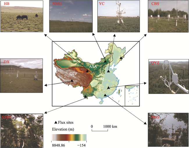
Figure 1 Overview of the three climatic regions of China

2.2 Data and processing

2.2.1 NPP data

The eddy flux data were obtained from China Flux observations (http://www.chinaflux.org/). We selected eight sites as representatives of different vegetation types (Figure 1): Changbai Mountain temperate Korean pine broad-leaved forest (CBS), Dinghushan subtropical evergreen broad-leaved forest (DHS), Dangxiong alpine meadow (DX), Haibei alpine meadow (HB), Qianyanzhou plantation (QYZ), Inner Mongolia temperate typical grassland (NMG), Xishuangbanna tropical rain forest (XSBN), and Yucheng warm temperate dry farmland (YC).
The eddy flux data provided the gross primary production (GPP) values during 2003- 2010. NPP can be calculated by the ratio of NPP to GPP (φ) (Waring et al., 1998). Theoretically, φ values vary with temperature and precipitation, but the changes in φ are relatively small (Maseyk et al., 2008; Zhang et al., 2009). The changes in φ can also be offset by physiological adaptation (Drake et al., 2016). In previous reports, φ is represented as a fixed value (Waring et al., 1998). In many models, φ is also a fixed value, such as in CASA (Potter et al., 1993) and Biome-BGC (Running and Hunt, 1993). A recent study confirmed that φ values probably vary from 0.4 to 0.6 (Landsberg et al., 2020). Therefore, to facilitate the calculation in this study, we used the parameters from the previous literature (Zhang et al., 2014b) to calculate the monthly NPP data of the eddy covariance sites. The φ values of different sites are shown in Table 1.
Table 1 Geographic coordinates, NPP/GPP values (φ), and vegetation types for the eddy covariance sites
Sites Longitude Latitude φ Types
CBS 128°06′E 42°24′N 0.5488 Forest
QYZ 115°03′E 26°44′N 0.4125 Forest
DHS 112°30′E 23°09′N 0.4125 Forest
XSBN 101°16′E 21°54′N 0.4125 Forest
NMG 116°18′E 44°08′N 0.4000 Grass
HB 101°20′E 37°40′N 0.5523 Grass
DX 91°03′E 30°29′N 0.5523 Grass
YC 116°38′E 36°58′N 0.5399 Crops

2.2.2 NDVI data

The NDVI data were obtained from the National Aeronautics and Space Administration (NASA) MOD13A3 product (https://search.Earthdata.nasa.gov/search). The spatial resolution was 1000 m × 1000 m and the temporal resolution was one month. The quality of this dataset is high (Beck et al., 2011), and the data have been widely used for vegetation dynamics research (Jin et al., 2020; Wei et al., 2020).

2.2.3 Climate data

The temperature and precipitation data from 2001 to 2017 were obtained from the National Earth System Science Data (http://loess.geodata.cn). The dataset was generated from the global 0.5° climate dataset released by the Climatic Research Unit (CRU) and the global high-resolution climate dataset released by WorldClim, downscaled in the Chinese region by the Delta spatial downscaling scheme with a spatial resolution of 1000 m × 1000 m. This product has been assessed using data from 496 meteorological observation stations, and the results were credible. The monthly solar radiation data were from NASA (https://mynasadata.larc.nasa.gov/thredds/catalog.html), with a spatial resolution of 1° × 1°. Finally, the bilinear interpolation method was used to resample the three types of data to 1000 m × 1000 m.

2.2.4 Surface reflectance data

The surface reflectance data were obtained from the NASA MOD09A1 product (https://search.Earthdata.nasa.gov/search), with a spatial resolution of 500 m × 500 m and a time resolution of eight days. The monthly data were resampled to 1000 m × 1000 m by the bilinear interpolation method.

2.2.5 Land cover type data

The land cover type data (2001-2017) were obtained from the NASA MCD12Q1 product (https://search.Earthdata.nasa.gov/search). The first classification scheme (International Geosphere-Biosphere Programme (IGBP)) has the best robustness and consistency (Liang et al., 2015). Therefore, we adopted the IGBP vegetation classification system, and our study used four vegetation types: cultivated land, woodland, grassland, and desert.

2.3 Methods

2.3.1 The CASA model

We used the improved CASA model to estimate the NPP of vegetation. The NPP considering the climatic time lag in calculation is called NPP_L, and calculated with the original model is called NPP_O.
The CASA model is a model based on light use efficiency (Potter et al., 1993; Field et al., 1995), driven by temperature, precipitation, solar radiation, surface reflectance, NDVI, and land cover data. The model is mainly determined by two variables, namely the photosynthetic effective radiation (APAR) absorbed by vegetation and the actual light use efficiency (ε). The formula is as follows (Eq. (1)):
$NPP\left( x,t \right)=APAR\left( x,t \right)\times \varepsilon \left( x,t \right)$
where APAR(x,t) represents the photosynthetically active radiation absorbed by pixel x in month t (MJ·m-2·month-1), and ε(x,t) represents the actual light use efficiency (gC·MJ-1) of pixel x in month t. The calculation formula of photosynthetic active radiation (APAR) absorbed by vegetation is as follows (Eq. (2)):
$APAR\left( x,t \right)=SOL\left( x,t \right)\times FPAR\left( x,t \right)\times 0.5$
where SOL(x,t) represents the total solar radiation of pixel x in month t; FPAR(x,t) represents the absorption ratio of the vegetation layer to the incident photosynthetically active radiation. FPAR(x,t) is calculated from Normalized Vegetation Index (NDVI) and Ratio Vegetation Index (RVI). Not directly related to vegetation type but will be affected by vegetation type; and 0.5 is a constant value, which represents the ratio of solar effective radiation available to vegetation to total solar radiation.
Light use efficiency ε(x,t) refers to the efficiency of vegetation converting the absorbed photosynthetically active radiation into organic matter, which is mainly affected by temperature and moisture. The calculation formula is as follows (Eq. (3)):
\[\varepsilon \left( x,t \right)={{T}_{\varepsilon 1}}\left( x,t \right)\times {{T}_{\varepsilon 2}}\left( x,t \right)\times {{W}_{\varepsilon }}\left( x,t \right)\times {{\varepsilon }_{\text{max}}}\]
where Tε1(x,t) and Tε2(x,t) represent the stress of low and high temperature on light use efficiency, respectively; Wε(x,t) is the water stress coefficient, reflecting the influence of water conditions; εmax is the maximum light use efficiency (gC MJ-1) in the ideal state, which varies greatly with different vegetation types. We determined the εmax values according to the previous literature.
Tε1(x,t) and Tε2(x,t) were calculated by the method of the original model, and the calculation formula is as follows (Eq. (4) and (5)):
${{T}_{\varepsilon 1}}\left( x,t \right)=0.8+0.02\times Topt\left( x \right)-0.0005\times {{\left[ Topt\left( x \right) \right]}^{2}}$
$\begin{align}& {{T}_{\varepsilon 2}}\left( x,t \right)=1.184/\left\{ 1+\text{exp}\left[ 0.2\times \left( Topt\left( x \right)-10-T\left( x,t \right) \right) \right] \right\}\times \\& \ \ \ \ \ \ \ \ \ \ \ \ \ \ \ \ 1/\left\{ 1+\text{exp}\left[ 0.3\times \left( -Topt\left( x \right)-10+T\left( x,t \right) \right) \right] \right\} \\\end{align}$
where Topt(x) is the optimum temperature for plant growth, which is defined as the monthly average temperature (℃) when the NDVI value reaches the highest value in a certain region within a year; when the monthly average temperature is less than or equal to -10℃, Tε1(x,t) takes 0. Tε2(x,t) represents the trend that the plant light energy utilization rate gradually decreases when the ambient temperature changes from the optimum temperature Topt(x) to high or low temperature.
Wε(x,t) was calculated by the method in the vegetation photosynthesis model (VPM), because the method in the original model is based on actual and potential evapotranspiration, which has great uncertainty. The detailed calculation process of Wε(x,t) was described in reference (Xiao et al., 2004).

2.3.2 Time-lag effects

Previous studies have suggested that the time lag of vegetation to climate is usually within three months (Rundquist and Harrington Jr, 2000; Anderson et al., 2010). Therefore, there were four values, i.e., 0, 1, 2, and 3 months in this study. Since the time-lag effect is related to the growth stage of vegetation, the lag period of different seasons was also considered. In this study, temperature, precipitation, and solar radiation data were independent variables, while NDVI data was dependent variables. In order to determine the time lag, we calculated the partial correlation coefficients (R) of all of these months, and then selected the lag month based on the maximum R (Wen et al., 2018). For instance, when calculating the time lag in winter (December, January, and February), there were three types of data in each grid, i.e., (NDVI-Dec, Tem-Dec), (NDVI-Jan, Tem-Jan), and (NDVI-Feb, Tem-Feb). Our study extended over a period of 17 years and, thus, each grid had 3 × 17 = 51 data points. Using these data, the partial correlation efficient of each grid was calculated. We assumed that the time lag was one month, and the data for each grid were as follows: (NDVI-Dec, Tem-Nov), (NDVI-Jan, Tem-Dec), and (NDVI-Feb, Tem-Jan), and the R value was calculated. The time lag was two or three months and so on. We compared the partial correlation coefficients for all of the grids at the time lag of 0, 1, 2, and 3 months, and then determined the time lag according to the largest values of R. For the determination of the time lag for temperature, we calculated the R for these values with the fixed values of precipitation and solar radiation. The time-lag calculation for other environmental factors and seasons was performed similarly. The formula of the partial correlation coefficient can be expressed as follows (Eq. (6)) (Wu et al., 2015):
\[r_{12,3\sim p}^{2}=\frac{R_{1(2,3,...p)}^{2}-R_{1(3,...p)}^{2}}{1-R_{1(3,...p)}^{2}}\]
where p is the number of factors. In this study, there were three factors, i.e., temperature, precipitation, and solar radiation. For example, during the calculation of the partial correlation coefficient of NDVI and temperature,\[{{r}_{12,3\sim p}}\]is the partial correlation coefficient of NDVI and temperature, which uses precipitation and radiation as the control variables. \[R_{1(2,3,\ldots p)}^{2}\]is the determination coefficient of the regression analysis of NDVI (variable 1) and temperature, precipitation, and radiation (variable (2~p));\[R_{1(3,\ldots p)}^{2}\]is the coefficient of determination of the regression analysis of NDVI (variable 1) and precipitation and radiation (variable (3-p)).
After the time lag of the climate factors was determined, the mean values were calculated of the meteorological data from the current month to the time lag months. For example, the lag period was n months, and the input temperature input into CASA model was the monthly average value of the previous n months and the current month. The calculation formula is as follows (Eq. (7)):
${{X}_{i}}=\frac{\mathop{\sum }_{t=i-n}^{i}{{x}_{t}}}{n}$
where Xi is the meteorological data of the nth month that finally participated in the calculation of the CASA model. n is the time lag. xt is the climate factor for month t.

2.3.3 Calculation of the annual change rate of NPP

We used least squares regression to analyze the spatiotemporal changes of NPP from 2002 to 2017. The calculated method is expressed as (Eq. (8)):
\[\text{ }\!\!~\!\!\text{ }slope=\frac{n\times \underset{n}{\overset{i=1}{\mathop{\mathop{\sum }^{}}}}\,i\times NP{{P}_{i}}-\underset{n}{\overset{i=1}{\mathop{\mathop{\sum }^{}}}}\,i\underset{n}{\overset{i=1}{\mathop{\mathop{\sum }^{}}}}\,NP{{P}_{i}}}{n\times \underset{n}{\overset{i=1}{\mathop{\mathop{\sum }^{}}}}\,{{i}^{2}}-{{\left( \underset{n}{\overset{i=1}{\mathop{\mathop{\sum }^{}}}}\,i \right)}^{2}}}\]
where slope refers to the interannual trend of NPP. NPPi is the NPP in year i.

3 Results

3.1 Time lag of the vegetation response to climate factors

During spring, the average the time lag of vegetation on temperature in spring was 0.93 months, with higher values in the QTP (1.18 months) and the ASA (1.09 months) (Figure 2). In summer, the average time lag was 1.20 months, with the highest value in the ASA (1.43 months). The average time lag in autumn was 1.73 months. The QTP (1.91 months) and the ASA (1.95 months) had higher values. In winter, the average time lag was 1.09 months, with a higher value on the QTP (1.22 months).
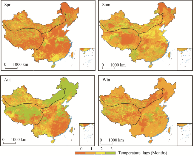
Figure 2 The average time lag of the vegetation response to temperature in different seasons during 2001-2017
There was a clear time lag in the vegetation response to precipitation (Figure 3), with the average values of 1.58, 1.38, 1.57, and 1.44 months in spring, summer, autumn, and winter. The greater time-lag months were for the EM in spring (1.79) and summer (1.45), while the QTP (1.72) and ASA (1.79) had larger time-lag months. The EM area showed a greater time lag (1.53 months) than the average value in winter.
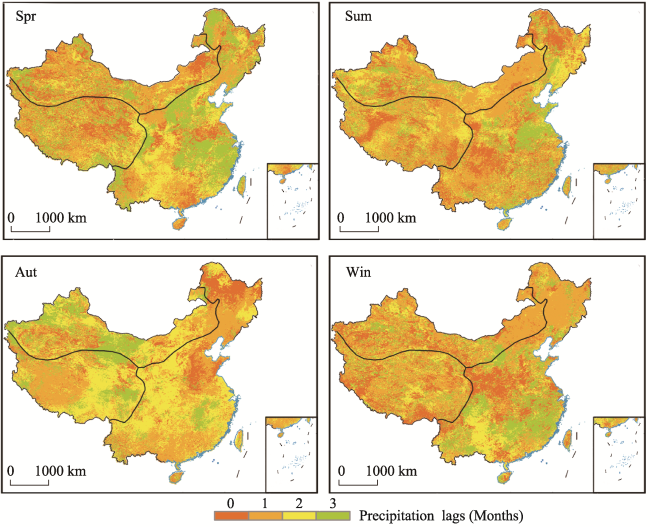
Figure 3 The average time lag of the vegetation response to precipitation in different seasons during 2001-2017
The average lag time of vegetation to solar radiation in spring was 2.35 months. During summer and autumn, the average time lag was 0.92 and 2.07 months. In winter, the average lag time was 0.97 months, with higher values in the QTP (1.20 months) and the ASA (1.06 months).
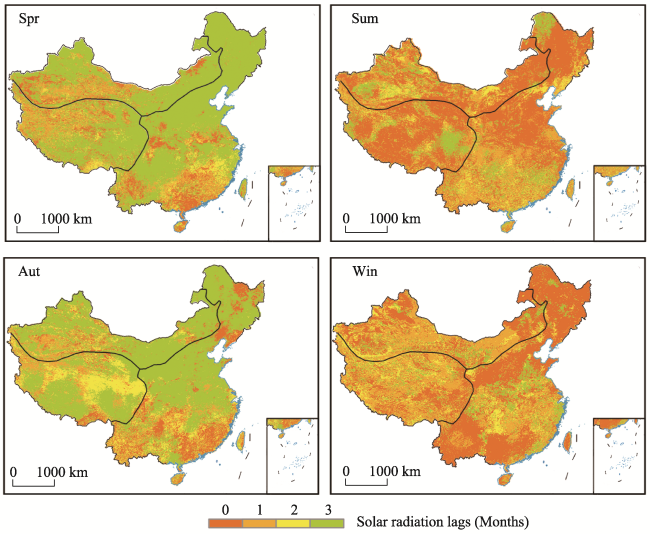
Figure 4 The averaged lag time of the vegetation response to solar radiation in different seasons during 2001-2017
The statistical analysis showed that the lag period of vegetation to solar radiation was the longest, followed by precipitation, with the lowest time lag being in relation to temperature (Table 2). For the different climate zones and vegetation types, the ASA and deserts of northwest China had the longest time-lag values for temperature. The EM, forests, and desert had the longest time-lag values for precipitation. The QTP and grasslands had the longest time-lag values for solar radiation.
Table 2 Time-lag period of climatic factors in the different climate zones and vegetation types
Temperature Precipitation Solar radiation
China 1.24 1.49 1.58
EM 1.11 1.53 1.50
QTP 1.30 1.49 1.69
ASA 1.40 1.43 1.60
Farmland 1.18 1.50 1.52
Forest 1.06 1.54 1.51
Grassland 1.26 1.42 1.67
Desert 1.45 1.54 1.59

3.2 NPP validation

Based on the eddy covariance data, we assessed the accuracy of the simulated NPP values using the CASA model with (NPP_L) and without (NPP_O) considering the time lag from 2002 to 2017. The R2 values between the measured and modeled NPP suggested that the accuracy of the NPP simulation was improved at seven sites (Figure 5). The R2 values increased by at least 0.05 for five sites. There was only one site (YC) with a lower R2 value when considering the time-lag effect.
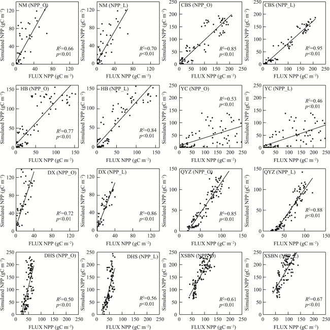
Figure 5 Comparison of the eddy flux site data and the simulated NPP during 2003-2010

3.3 Effects of the time lag on simulated NPP

3.3.1 Impact on the monthly NPP

In spring (March-May), the NPP difference in the eastern region is larger than that in the other two regions, and NPP_O>NPP_L, this situation peaks in May, and weakens after entering summer (June-August), and finally in most parts of China, it is NPP_O<NPP_L. This continues until the end of the fall (September-November). In autumn, most parts of the country still showed NPP_O<NPP_L, and the performance in the eastern part was more obvious. After entering winter (December-February), the time lag has the least impact on NPP, and the gap between NPP_O and NPP_L is about 5 m in most parts of the China time lag (Figure 6).
Figure 6 Average monthly difference in NPP_L minus NPP_O from January to December 2001-2017
During 2001-2017, the overall effects of the time lag on the monthly NPP showed that the vegetation growth season was slightly changed in spring. The most obvious change is that the growing seasons increased considerably, and the NPP values during August-November were higher than those of the original model that did not consider the time-lag effects (Figure 7).
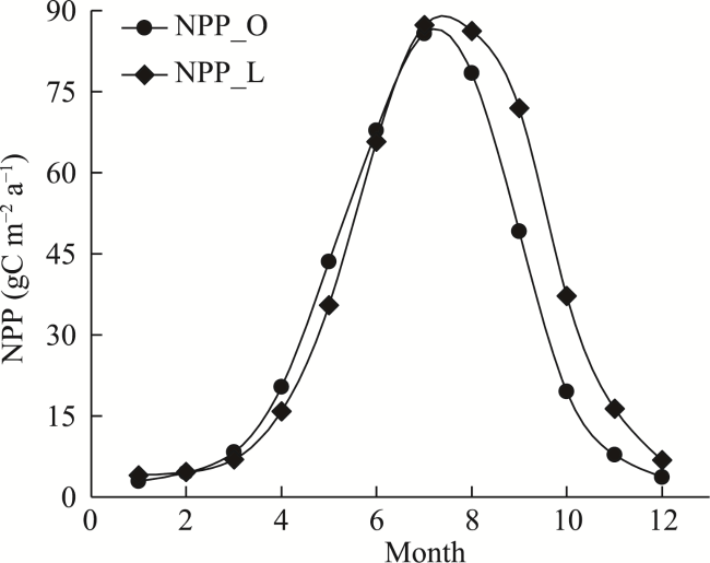
Figure 7 The average monthly changes in NPP from NPP_O and NPP_L during 2001-2017

3.3.2 Impact on the seasonal NPP

At the seasonal scale, there were only small differences in the NPP values between NPP_O and NPP_L (Figure 8). The NPP values from NPP_O were 24.84% higher than those of NPP_L in spring. In autumn, the NPP_O values were 38.74% lower than those of NPP_L (Figure 9).
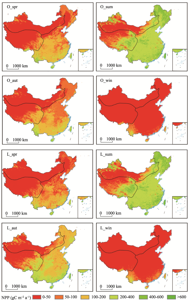
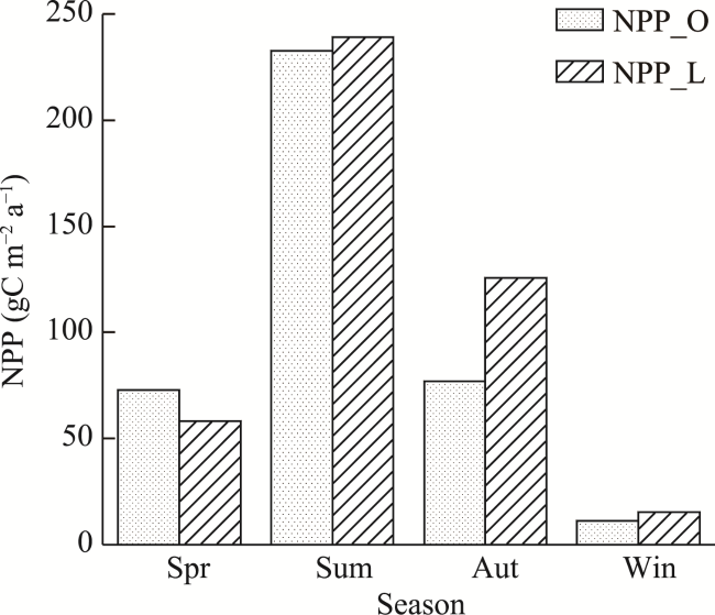
Figure 8 The average seasonal NPP values from NPP_O and NPP_L during 2001-2017 (O indicates the simulated NPP using the model without consideration of time-lag effects, and L indicates the simulated NPP values using the model that considered time-lag effects; spr, sum, aut, and win are abbreviations for the respective seasons.)
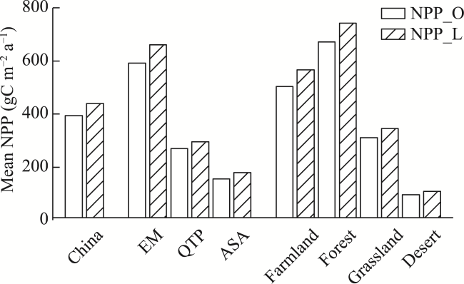
Figure 9 The average seasonal NPP values from NPP_O and NPP_L for China’s terrestrial ecosystems during 2001-2017 (O indicates the simulated NPP using the model without consideration of time-lag effects, and L indicates the simulated NPP values using the model that considered time-lag effects; spr, sum, aut, and win are abbreviations for the respective seasons.)

3.3.3 Impact on the annual NPP

The average and total amount of NPP_L for China’s terrestrial ecosystems were 438.47 gC m-2 a-1 and 3.977 PgC a-1, respectively. The total NPP values from NPP_L were 11.37% higher than those from NPP_O (Figure 10). The NPP_O values were similar to those from NPP_L in 23.11% of the total areas (ranging from -10 to 10 gC m-2), while 74.62% of the areas had lower NPP values and only 2.27% of the areas had higher NPP values from the NPP_L model (Figure 10).
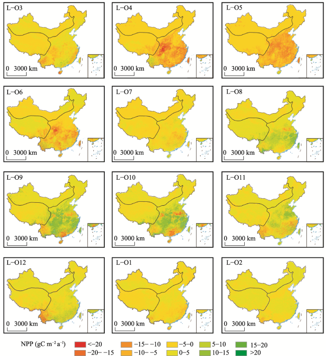
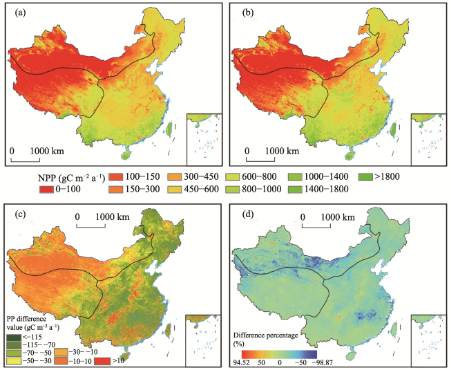
Figure 10 Comparison between the average annual NPP values from the NPP_O and NPP_L models during 2001-2017 (Spatial distribution of the NPP values from NPP_O (a) and NPP_L (b); the absolute (c) and relative (d) differences between the NPP values from the NPP_O minus NPP_L models)
At the annual scale, the greatest impact of the time lag on NPP was found in the ASA and desert areas. For the calculated NPP using the model considering the time-lag effects, the annual NPP values were 14.30% and 13.68% higher than those of the model without consideration of time-lag effects. The QTP and forest areas had minimal impacts, and the NPP values from NPP_L were 9.09% and 10.40% higher than those from NPP_O (Figure 11).
Figure 11 Comparison of the annual NPP values from NPP_O and NPP_L of China’s terrestrial ecosystems during 2001-2017 (EM indicates the eastern monsoon region, ASA indicates the northwest arid and semi-arid region, and QTP indicates the Qinghai-Tibet Plateau.)
The time lag effect has little effect on the interannual variation trend of NPP from 2001 to 2017. Considering the time lag effect, the area that passed the significance test (p < 0.05) accounted for 27.00%, which was 6.72 percentage points higher. than the case where the time lag effects are not considered (Figure 12).
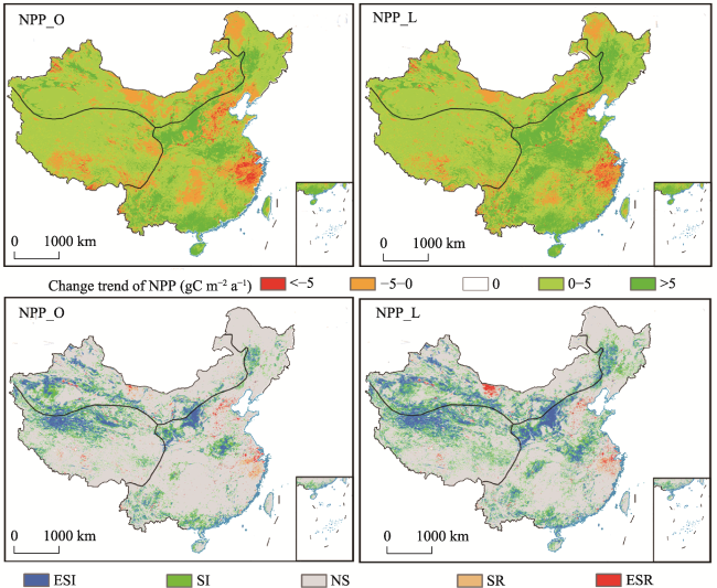
Figure 12 Changing trends and significant test of the annual NPP_O and NPP_L simulated NPP values from 2001 to 2017 (ESI and SI indicate a significant increasing trend at p < 0.01 and p < 0.05; ESR and ER indicate a significant decreasing trend at p < 0.01 and p < 0.05.)

4 Discussion

4.1 Time-lag periods

Vegetation growth is very sensitive to temperature fluctuations (de Jong et al., 2013), and its response to temperature is faster than precipitation. In this study, the lag period of temperature was the shortest (1.24 months). Overall, the vegetation temperature lag period in autumn was the longest (1.73 months). This may be due to the fact that plants have some physiological mechanisms to adapt to cold temperature, and thereby prolong the growth period of vegetation (Damberg and AghaKouchak, 2014; Mulder et al., 2017).
The precipitation time lag was largely greater than one month in our study. Previous reports have suggested that the response of vegetation growth usually lags precipitation by one month (Gessner et al., 2013). Precipitation and factors such as VPD, PET of the air and the available water in the soil affected by precipitation are usually important factors in regulating global vegetation growth (Liu et al., 2013). It is worth noting that the lag period of precipitation in the ASA was the longest (1.79 months) in autumn. In the ASA region, the precipitation was high while drought events likely occurred in autumn. This finding probably reveals the fact that the plants in this area have good adaptability to water stress and can tolerate water shortages for a period of time (Anderegg et al., 2015; Wen et al., 2019). This idea is also supported by the short time lag in summer, during which precipitation was high, meaning that the amount of precipitation is sufficient for vegetation growth in summer.
The time lag of vegetation to solar radiation was the longest (1.58 months), which is consistent with previous findings that most vegetation types have the time lag of more than a month (Wu et al., 2015). There were differences in the time-lag periods among different climatic zones and vegetation types. For example, the QTP (1.69 months) and grassland (1.67 months) had the longer time lag periods than other climatic zones and vegetation types in spring. The QTP and grassland in China are mainly characterized by higher solar radiation (Li et al., 2011), indicating that solar radiation should not be a limited factor for vegetation growth. Therefore, this finding likely suggests that the vegetation growth in spring was affected by other factors such as precipitation and temperature (Nemani et al., 2003; de Jong et al., 2013).

4.2 Effects of the time lag on the simulated NPP using the CASA model

The statistical analysis between the modeled NPP and the field-observed NPP using eddy covariance showed that the model with the consideration of the time lag improved the simulation accuracy, and the R2 increased by approximately 10% for six of the eight observed sites. There was only one site, namely YC, that had a lower R2 value in comparison to the model without the consideration of time-lag effects. This could be attributed to the fact that this site comprises crop land, and human management plays a controlling role with regard to NPP.
The simulated NPP in China’s terrestrial ecosystems from the model with consideration of time-lag effects was higher than that of the model without consideration of time-lag effects. This finding is in agreement with our expectations. The time lag of the vegetation response to climate change suggests that the accumulating effects of climate change promote vegetation growth (Wen et al., 2019), unless extreme events such as drought or high temperature occur, which are damaging to vegetation (Wang et al., 2015). For the monthly changes in NPP, we found that the time-lag effects were not obvious before July; this can be explained by the fact that China has a simultaneous pattern in precipitation and temperature, and thus plant growth is prolonged after July (Lian et al., 2021). Unlike with other seasons, the simulated NPP showed a slight decrease after the consideration of the time lag effects; this result coincides with previous reports that vegetation growth can be affected by the climate conditions in the previous winter season (Shen et al., 2011; Chen et al., 2015).

4.3 Future research priorities

Currently, statistical analysis is commonly used between vegetation indices such as the NDVI to calculate the time lag (Wu et al., 2015; Tei and Sugimoto, 2018; Ding et al., 2020), and little is known about the physiological mechanisms behind the time lag of the vegetation response to climate variables. More attention should be paid to plant physiology to address the biological mechanisms of the time lag of vegetation growth in the future.
There are some shortcomings and uncertainties in this study. Similar to previous reports, we calculated the time lag on a monthly scale due to data limitations. Although this method is widely used, it is obvious that analysis of the time lag on a closer time scale is needed in the future. We also assumed that the relationship between vegetation NDVI and meteorological factors is linear, despite the fact that vegetation phenology is complicated (Brando et al., 2010). Therefore, future studies that focused on calculation methods for time-lag effects are required. Based on the statistical analysis, we revealed that the vegetation response to climate variables has the time lag; however, the effects of non-climatic factors such as nitrogen deposition and mineralization, extreme climate, human activities, and natural disturbances were not quantified. In addition, the comparison with eddy covariance sites showed that the accuracy of the simulated NPP from the model with the consideration of time-lag effects was improved. However, the validation data still comprise only a small sample, and more field-observed data are required for a better understanding of the NPP at a regional scale.

5 Conclusion

In this study, NDVI and climate data were used to calculate the time-lag effects of vegetation growth to temperature, precipitation, and solar radiation in different seasons. The CASA model was then used to simulate the NPP considering time lag in China from 2002 to 2017. The results show that these climate factors have obvious time-lag effects on vegetation growth, with considerable temporal and spatial differences. The CASA model, with the consideration of time-lag effects, improves the accuracy of NPP simulation. From 2002 to 2017, the NPP of China’s terrestrial ecosystems was probably underestimated without the consideration of time-lag effects. However, the time-lag effects were obvious after the summer. Taken together, our results highlight the importance of time-lag effects on vegetation growth, and provide a new framework to improve the accuracy of simulated NPP values using different models.
[1]
Anderegg W R, Schwalm C, Biondi F et al., 2015. Pervasive drought legacies in forest ecosystems and their implications for carbon cycle models. Science, 349: 528-532.

DOI PMID

[2]
Anderson L O, Malhi Y, Aragão L E et al., 2010. Remote sensing detection of droughts in Amazonian forest canopies. New Phytologist, 187: 733-750.

DOI PMID

[3]
Beck H E, Mcvicar T R, Van Dijk A I et al., 2011. Global evaluation of four AVHRR-NDVI data sets: Intercomparison and assessment against Landsat imagery. Remote Sensing of Environment, 115: 2547-2563.

DOI

[4]
Brando P M, Goetz S J, Baccini A et al., 2010. Seasonal and interannual variability of climate and vegetation indices across the Amazon. Proceedings of the National Academy of Sciences, 107: 14685-14690.

DOI

[5]
Chen T, De Jeu R, Liu Y et al., 2014. Using satellite based soil moisture to quantify the water driven variability in NDVI: A case study over mainland Australia. Remote Sensing of Environment, 140: 330-338.

DOI

[6]
Chen X, An S, Inouye D W et al., 2015. Temperature and snowfall trigger alpine vegetation green-up on the world's roof. Global Change Biology, 21: 3635-3646.

DOI PMID

[7]
Damberg L, Aghakouchak A, 2014. Global trends and patterns of drought from space. Theoretical Applied Climatology, 117: 441-448.

DOI

[8]
Davis M B, 1989. Lags in vegetation response to greenhouse warming. Climatic Change, 15: 75-82.

DOI

[9]
De Jong R, Schaepman M E, Furrer R et al., 2013. Spatial relationship between climatologies and changes in global vegetation activity. Global Change Biology, 19: 1953-1964.

DOI PMID

[10]
Ding Y, Li Z, Peng S, 2020. Global analysis of time-lag and -accumulation effects of climate on vegetation growth. International Journal of Applied Earth Observation Geoinformation, 92: 102179.

DOI

[11]
Drake J E, Tjoelker M G, Aspinwall M J et al., 2016. Does physiological acclimation to climate warming stabilize the ratio of canopy respiration to photosynthesis? New Phytologist, 211: 850-863.

DOI PMID

[12]
Field C B, Behrenfeld M J, Randerson J T et al., 1998. Primary production of the biosphere: Integrating terrestrial and oceanic components. Science, 281: 237-240.

DOI PMID

[13]
Field C B, Randerson J T, Malmström C M, 1995. Global net primary production: Combining ecology and remote sensing. Remote Sensing of Environment, 51: 74-88.

DOI

[14]
Fu Y H, Piao S, Zhao H et al., 2014. Unexpected role of winter precipitation in determining heat requirement for spring vegetation green-up at northern middle and high latitudes. Global Change Biology, 20: 3743-3755.

DOI PMID

[15]
Gessner U, Naeimi V, Klein I et al., 2013. The relationship between precipitation anomalies and satellite-derived vegetation activity in Central Asia. Global Planetary Change, 110: 74-87.

DOI

[16]
Jin H, Bao G, Chen J et al., 2020. Modifying the maximal light-use efficiency for enhancing predictions of vegetation net primary productivity on the Mongolian Plateau. International Journal of Remote Sensing, 41: 3740-3760.

DOI

[17]
Kong D, Miao C, Wu J et al., 2020. Time lag of vegetation growth on the Loess Plateau in response to climate factors: Estimation, distribution, and influence. Science of The Total Environment, 744: 140726.

DOI

[18]
Landsberg J J, Waring R H, Williams M, 2020. The assessment of NPP/GPP ratio. Tree Physiology, 40: 695-699.

DOI PMID

[19]
Leroy S A, Arpe K, Mikolajewicz U, 2011. Vegetation context and climatic limits of the Early Pleistocene hominin dispersal in Europe. Quaternary Science Reviews, 30: 1448-1463.

DOI

[20]
Li C, Sun H, Wu X et al., 2020. An approach for improving soil water content for modeling net primary production on the Qinghai-Tibetan Plateau using Biome-BGC model. Catena, 184: 104253.

DOI

[21]
Li H, Ma W, Lian Y et al., 2011. Global solar radiation estimation with sunshine duration in Tibet, China. Renewable Energy, 36: 3141-3145.

DOI

[22]
Lian X, Piao S, Chen A et al., 2021. Seasonal biological carryover dominates northern vegetation growth. Nature Communications, 12: 1-10.

DOI

[23]
Liang D, Zuo Y, Huang L et al., 2015. Evaluation of the consistency of MODIS Land Cover Product (MCD12Q1) based on Chinese 30 m GlobeLand30 datasets: A case study in Anhui Province, China. ISPRS International Journal of Geo-Information, 4: 2519-2541.

DOI

[24]
Lieth H, 1975. Modeling the primary productivity of the world. Primary Productivity of the Biosphere: 237-263.

[25]
Liu Q, Fu Y H, Zeng Z et al., 2016. Temperature, precipitation, and insolation effects on autumn vegetation phenology in temperate China. Global Change Biology, 22: 644-655.

DOI PMID

[26]
Liu Y Y, Van Dijk A I, Mccabe M F et al., 2013. Global vegetation biomass change (1988-2008) and attribution to environmental and human drivers. Global Ecology Biogeography, 22: 692-705.

DOI

[27]
Maseyk K, Grünzweig J M, Rotenberg E et al., 2008. Respiration acclimation contributes to high carbon-use efficiency in a seasonally dry pine forest. Global Change Biology, 14: 1553-1567.

DOI

[28]
Mulder C P, Iles D T, Rockwell R F, 2017. Increased variance in temperature and lag effects alter phenological responses to rapid warming in a subarctic plant community. Global Change Biology, 23: 801-814.

DOI PMID

[29]
Nemani R R, Keeling C D, Hashimoto H et al., 2003. Climate-driven increases in global terrestrial net primary production from 1982 to 1999. Science, 300: 1560-1563.

PMID

[30]
O'sullivan M, Smith W K, Sitch S et al., 2020. Climate-driven variability and trends in plant productivity over recent decades based on three global products. Global Biogeochemical Cycles, 34: e2020GB006613.

[31]
Parton W, Scurlock J, Ojima D et al., 1993. Observations and modeling of biomass and soil organic matter dynamics for the grassland biome worldwide. Global Biogeochemical Cycles, 7: 785-809.

DOI

[32]
Peters R L, Speich M, Pappas C et al., 2019. Contrasting stomatal sensitivity to temperature and soil drought in mature alpine conifers. Plant Cell Environment, 42: 1674-1689.

DOI

[33]
Piao S, Fang J, Zhou L et al., 2005. Changes in vegetation net primary productivity from 1982 to 1999 in China. Global Biogeochemical Cycles, 19.

[34]
Potter C S, Randerson J T, Field C B et al., 1993. Terrestrial ecosystem production: A process model based on global satellite and surface data. Global Biogeochemical Cycles, 7: 811-841.

DOI

[35]
Rumpf S B, Hülber K, Wessely J et al., 2019. Extinction debts and colonization credits of non-forest plants in the European Alps. Nature Communications, 10: 1-9.

DOI

[36]
Rundquist B C, Harrington Jr J A, 2000. The effects of climatic factors on vegetation dynamics of tallgrass and shortgrass cover. GeoCarto International, 15: 33-38.

DOI

[37]
Running S W, Hunt E R, 1993. Generalization of a forest ecosystem process model for other biomes, BIOME-BGC, and an application for global-scale models. In: Ehleringer J R, Field C B. Scaling Physiological Processes. San Diego: Academic Press: 141-158.

[38]
Saatchi S, Asefi-Najafabady S, Malhi Y et al., 2013. Persistent effects of a severe drought on Amazonian forest canopy. Proceedings of the National Academy of Sciences, 110: 565-570.

DOI

[39]
Shen M, Tang Y, Chen J et al., 2011. Influences of temperature and precipitation before the growing season on spring phenology in grasslands of the central and eastern Qinghai-Tibetan Plateau. Agricultural Forest Meteorology, 151: 1711-1722.

DOI

[40]
Sun Q, Li B, Zhou C et al., 2017. A systematic review of research studies on the estimation of net primary productivity in the Three-River Headwater Region, China. Journal of Geographical Sciences, 27(2): 161-182.

DOI

[41]
Tei S, Sugimoto A, 2018. Time lag and negative responses of forest greenness and tree growth to warming over circumboreal forests. Global Change Biology, 24: 4225-4237.

DOI PMID

[42]
Wang X, Piao S, Xu X et al., 2015. Has the advancing onset of spring vegetation green-up slowed down or changed abruptly over the last three decades. Global Ecology Biogeography, 24: 621-631.

DOI

[43]
Waring R, Landsberg J, Williams M, 1998. Net primary production of forests: A constant fraction of gross primary production. Tree Physiology, 18: 129-134.

PMID

[44]
Wei W, Guo Z, Zhou L et al., 2020. Assessing environmental interference in northern China using a spatial distance model: From the perspective of geographic detection. Science of The Total Environment, 709: 136170.

DOI

[45]
Wen Y, Liu X, Pei F et al., 2018. Non-uniform time-lag effects of terrestrial vegetation responses to asymmetric warming. Agricultural Forest Meteorology, 252: 130-143.

DOI

[46]
Wen Y, Liu X, Xin Q et al., 2019. Cumulative effects of climatic factors on terrestrial vegetation growth. Journal of Geophysical Research: Biogeosciences, 124: 789-806.

[47]
Wu D, Zhao X, Liang S et al., 2015. Time-lag effects of global vegetation responses to climate change. Global Change Biology, 21: 3520-3531.

DOI PMID

[48]
Xiao X, Hollinger D, Aber J et al., 2004. Satellite-based modeling of gross primary production in an evergreen needleleaf forest. Remote Sensing of Environment, 89: 519-534.

DOI

[49]
Yuan Q, Wu S, Zhao D et al., 2014. Modeling net primary productivity of the terrestrial ecosystem in China from 1961 to 2005. Journal of Geographical Sciences, 24(1): 3-17.

DOI

[50]
Yuan W, Liu S, Zhou G et al., 2007. Deriving a light use efficiency model from eddy covariance flux data for predicting daily gross primary production across biomes. Agricultural Forest Meteorology, 143: 189-207.

DOI

[51]
Yunus A P, Fan X, Tang X et al., 2020. Decadal vegetation succession from MODIS reveals the spatio-temporal evolution of post-seismic landsliding after the 2008 Wenchuan earthquake. Remote Sensing of Environment, 236: 111476.

DOI

[52]
Zhang Y, Qi W, Zhou C et al., 2014a. Spatial and temporal variability in the net primary production of alpine grassland on the Tibetan Plateau since 1982. Journal of Geographical Sciences, 24: 269-287.

DOI

[53]
Zhang Y, Xu M, Chen H et al., 2009. Global pattern of NPP to GPP ratio derived from MODIS data: Effects of ecosystem type, geographical location and climate. Global Ecology Biogeography, 18: 280-290.

DOI

[54]
Zhang Y, Yu G, Yang J et al., 2014b. Climate-driven global changes in carbon use efficiency. Global Ecology Biogeography, 23: 144-155.

DOI

Outlines

/