Research Articles

The spatiotemporal scale effect on vegetation interannual trend estimates based on satellite products over Qinghai-Tibet Plateau

  • MA Dujuan , 1 ,
  • WU Xiaodan , 1, * ,
  • WANG Jingping 1 ,
  • MU Cuicui 1, 2, 3
Expand
  • 1. College of Earth and Environmental Sciences, Lanzhou University, Lanzhou 730000, China
  • 2. Southern Marine Science and Engineering Guangdong Laboratory (Zhuhai), Zhuhai 611930, Guangdong, China
  • 3. University Cooperation of Polar Research, Beijing 100875, China
*Wu Xiaodan (1987–), PhD and Professor, specialized in the validation of quantitative remote sensing products over heterogeneous land surfaces. E-mail:

Ma Dujuan (1994-), Master Candidate, specialized in the scale effect of quantitative remote sensing products and vegetation remote sensing. E-mail:

Received date: 2022-03-28

  Accepted date: 2022-12-01

  Online published: 2023-05-11

Supported by

The Second Tibetan Plateau Scientific Expedition and Research Program(STEP)(2019QZKK0605)

National Natural Science Foundation of China(42071296)

Abstract

The trend estimate of vegetation change is essential to understand the change rule of the ecosystem. Previous studies were mainly focused on quantifying trends or analyzing their spatial distribution characteristics. Nevertheless, the uncertainties of trend estimates caused by spatiotemporal scale effects have rarely been studied. In response to this challenge, this study aims to investigate spatiotemporal scale effects on trend estimates using Moderate-Resolution Imaging Spectroradiometer (MODIS) Normalized Difference Vegetation Index (NDVI) and Gross Primary Productivity (GPP) products from 2001 to 2019 in the Qinghai-Tibet Plateau (QTP). Moreover, the possible influencing factors on spatiotemporal scale effect, including spatial heterogeneity, topography, and vegetation types, were explored. The results indicate that the spatial scale effect depends more on the dataset with a coarser spatial resolution, and temporal scale effects depend on the time span of datasets. Unexpectedly, the trend estimates on the 8-day and yearly scale are much closer than that on the monthly scale. In addition, in areas with low spatial heterogeneity, low topography variability, and sparse vegetation, the spatiotemporal scale effect can be ignored, and vice versa. The results in this study help deepen the consciousness and understanding of spatiotemporal scale effects on trend detection.

Cite this article

MA Dujuan , WU Xiaodan , WANG Jingping , MU Cuicui . The spatiotemporal scale effect on vegetation interannual trend estimates based on satellite products over Qinghai-Tibet Plateau[J]. Journal of Geographical Sciences, 2023 , 33(5) : 924 -944 . DOI: 10.1007/s11442-023-2113-y

1 Introduction

Detecting the changing trend of vegetation is meaningful for quantifying and understanding the effect of carbon cycle and climate change (Ichii et al., 2002; Mu et al., 2013). Vegetation Index (VI) and GPP are two variables to reflect vegetation dynamic change from the aspects of greenness and carbon fixation. Remote sensing shows an absolute advantage in assessing vegetation status due to its large spatial coverage and periodical updating (Ghazaryan, 2015). Moreover, it provides vegetation products with different spatial, temporal, and spectral resolutions, offering a comprehensive understanding of vegetation change status from different perspectives (Cheng et al., 2003).
Nevertheless, the trends are usually inconsistent over the same area when different remote sensing datasets were used. For example, Fensholt et al. (2009) compared NDVI trends derived from AVHRR GIMMS, SPOT VGT, and MODIS TERRA in the Sahel from 2001 to 2009 and found that the three trends were not identical. SPOT VGT showed a higher positive trend than the other two datasets. AVHRR GIMMS NDVI trend was similar to Terra MODIS in the semi-arid domain but showed a higher positive trend than Terra MODIS in the humid region. Alcaraz et al. (2010) compared NDVI trends of GIMMS (AVHRR 8 km dataset) and CCRS (AVHRR 1 km dataset) in burned and unburned areas. It was found that CCRS NDVI showed an increasing trend in all burned domains and half of the unburned domain, but GIMMS NDVI did not capture the increasing trend and even showed a declining trend in the burned area ten years after the fire. Yu et al. (2013) detected NDVI trends in Tibetan Plateau using AVHRR, SPOT, and MODIS datasets. The results indicated that AVHRR NDVI showed a decreasing trend from the late 1990s, while SPOT and MODIS showed slight increase trends. The discrepancy of the trends estimated from different datasets poses a great challenge to draw definite conclusions about the real status of the environment and its response to climate change.
Several factors such as the different sensor types (Tian et al., 2015), satellite drift (Fensholt et al., 2009), trend detection algorithm (Wu et al., 2021), and the spatiotemporal scale effects (Chen et al., 2007; Zhao et al., 2009; Alcaraz et al., 2010; Beck et al., 2011) are considered to be responsible to these discrepancies. Despite the various kinds of error sources, this study focuses on the spatiotemporal scale effects on trend estimates and their influence characteristics, because few articles provide a systematic analysis of this issue and we are far from having a complete understanding of this crucial phenomenon.
We conducted a systematic and quantitative analysis of spatiotemporal scale effects on trend estimates of vegetation based on satellite products over QTP. To eliminate the influences of different sensors and trend detection algorithms, the same trend detection algorithm and the satellite products with different spatiotemporal scales from the same sensors were utilized. Specifically, MODIS NDVI products derived from Terra were used to explore spatial scale effects due to their various spatial resolutions (i.e., 250 m, 500 m, 1000 m, and 0.05°). By contrast, the MODIS GPP products (i.e., MOD17A2H) were used to explore temporal scale effects because of their higher temporal resolution of 8-day, creating favorable conditions for simulating datasets with different temporal resolutions.
The primary objective of this study is to deepen the understanding and consciousness of the spatiotemporal scale effects on trend detection results of vegetation change, and thereby help to remove the artificial trend from the observed trend. Specifically, this paper develops around three questions: (1) How does spatiotemporal scale effect affect trend estimates? (2) What factors (i.e., vegetation type, spatial heterogeneity, elevation, slope, aspect, and terrain variability) influence or determine spatiotemporal scale effects? (3) Which scale is favorable to detect change trends of vegetation surfaces? This paper starts by describing the study area and experimental data (Section 2). Section 3 explains the trend detection method as well as the methods of exploring spatiotemporal scale effects. Section 4 provides the results and discussions of spatiotemporal scale effects and their influence characteristics. Finally, a brief conclusion is summarized in Section 5.

2 Study area and experimental data

2.1 Study area

QTP covers almost one-fifth of China’s territory (Li et al., 2020) within the geographic area between 25.9°-40.0°N and 73.4°-104.3°E (Figure 1). The elevation of QTP is generally between 3000 m and 5000 m, which features the highest average altitude (about 4000 m) in the world and thus is called the “Roof of the World”. It has diverse land cover types due to its complex topography and unique climate. As shown in Figure 1, the dominant vegetation type is grassland, which is mainly distributed in the southwest, middle, and east of the QTP. Other vegetation types (i.e., forests, shrublands, savannas, and croplands) are scattered in the southeast boundary of QTP.
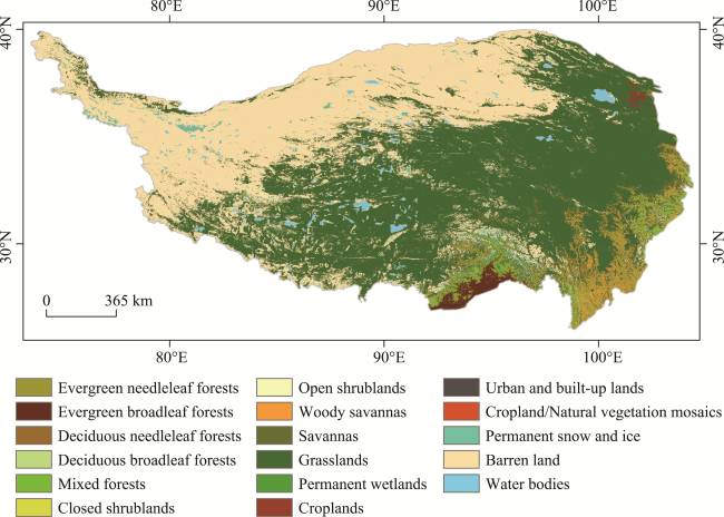
Figure 1 Land cover types of the Qinghai-Tibet Plateau
QTP was selected for the following reasons. First, it is more sensitive to climate change than other areas due to the biological limit (Liu et al., 2014), and thus became a hot area of climate change research (Zhang et al., 2019, Yuan et al., 2021). Second, the topography of QTP is complex (Wen et al., 2022), showing a trend of the east lower than the west in general, and such a distinctive terrain provides ideal conditions for detecting the effects of topography on spatiotemporal scale effects. Third, the vegetation types (Figure 1) on the QTP are enriched due to the difference in climate and topography, providing excellent suitability for detecting the effects of vegetation types on spatial scale effects. Last but not least, QTP has various climate types, and thus represents most of the climate zones on the global (Liu et al., 2012).

2.2 Data

2.2.1 Vegetation products

MODIS VI products are produced at 250 m (MOD13Q1), 500 m (MOD13A1), 1000 m (MOD13A2), and 0.05 deg (~5000 m) (MOD13C1) spatial resolutions currently, providing ideal datasets for exploring spatial scale effects on trend estimates. Standard pre-processings in generating these MODIS VI products include cloud pixels removal, atmospheric correction of aerosol, and the composting process in which the highest VI value from a series of multi-temporal images within 16-day periods is retained for each pixel location in order to reduce the effect of cloud and atmosphere contamination (Fagua and Ramsey, 2019). The NDVI products in growing seasons (160-240 days of year) were extracted from 2001 to 2019 to analyze the NDVI change. In order to make NDVI trend estimates comparable among different spatial resolutions, the results derived on fine resolutions were re-sampled to the corresponding coarser resolution.
MODIS GPP product, MOD17A2H, has been widely used in exploring the terrestrial ecosystem’s carbon cycle (Xia et al., 2015; Zhu et al., 2018). The retrieval algorithm of MOD17A2H is based on the Light Use Efficiency (LUE) model (Monteith, 1972):
$GPP\text{=}\varepsilon \times \text{fPAR}\times \text{PAR}$
where ɛ means the LUE within the defined period of time, fPAR is the fraction of absorbed photosynthetically-active radiation, and PAR represents the photosynthetic active radiation. The pixel size of this product is 500 m, and the temporal resolution is 8-day. Three commonly used temporal scales (including 8-day, monthly, and yearly scales) were utilized to test the temporal scale effects of trend estimates of GPP. Monthly and yearly scale datasets were calculated by temporally aggregating MOD17A2H in the corresponding temporal window.

2.2.2 Auxiliary data

In order to explore the relationship between spatial heterogeneity and spatial scale effects, NDVI data derived from Landsat 8 was utilized to calculate the spatial heterogeneity of NDVI within different coarse pixel scales. Specifically, the standard deviation of all Landsat 8 NDVI pixels within a coarse pixel was calculated to represent the spatial heterogeneity within the coarse pixel scale.
Land cover data were employed to investigate how spatiotemporal scale effects of trend estimates of vegetation change vary with vegetation types. Moderate Resolution Imaging Spectroradiometer Land Cover Type (MCD12Q1) product was employed in this study due to its wide acceptance. It provides global land cover type data at a spatial resolution of 500 m and a temporal resolution of 1-year based on the supervised classification of MODIS reflectance data with six different classification schemes. The Annual International Geosphere-Biosphere Programmer (IGBP) classification method was utilized to extract vegetation regions and differentiate vegetation types due to its better accuracy and widespread acceptance (Liang et al., 2015). The filling data of MCD12Q1 were removed before vegetation extraction in order to remove their effect on results. Furthermore, MCD12Q1 product was re-sampled to the corresponding coarser spatial resolution in order to ensure the accuracy of vegetation extraction.
Shuttle Radar Topography Mission (SRTM) dataset provides DEM data at a nearly global scope with a spatial resolution of 90 m. Data voids have been filled for ease of use. In this study, the elevation, slope, aspect, and topography variability were derived using this dataset in order to investigate their relationship with spatiotemporal scale effects. The slope and aspect were calculated using the corresponding function in Google Earth Engine (GEE), which were then re-sampled to the spatial resolution of NDVI trend estimates. It is noteworthy that the aspect values < 45° and > 315° were masked to avoid the influence of shadow (Anderson et al., 2020). For each coarser pixel of NDVI estimates, the topography variability was indicated by the standard deviation of elevations of all SRTM pixels within its spatial extent.

3 Methods

The primary goal of this study is to explore the spatiotemporal scale effects on trend estimates based on long-time series satellite products. Methods are described here from two aspects: trend detection technique and spatiotemporal scale effects exploration.

3.1 Trend detection

In order to determine the directions and rates of change, a pixel-based simple linear regression was applied, in which time was the independent variable while NDVI or GPP was the dependent variable. Using simple linear regression to estimate a trend from a time series is a practice widespread in the remote sensing literature (De Beurs et al., 2009; Fensholt et al., 2012; Liu et al., 2014). More importantly, different from non-linear methods, the results of the simple linear regression are easy to interpret and compare between different datasets (Fensholt et al., 2009).
In this study, both the satellite data and the linear regression function were provided by GEE, which is a cloud-based computing platform for planetary-scale data analysis, mapping, and modeling due to its free access to numerous global datasets and advanced computational capabilities (Gorelick et al., 2017). GEE was employed in this study for the following reasons: first, it provides almost all of the MODIS NDVI and GPP datasets and the auxiliary datasets such as land cover and DEM; second, it enables the rapid exploration and access of long time series datasets; third, it provides a library of functions (e.g., linear regression function, slope, and aspect functions) which are applied for data display and analysis.

3.2 Spatiotemporal scale effects

In order to quantify spatial scale effects on trend estimates, the NDVI trends were first calculated via linear regression based on the satellite datasets with different spatial resolutions. To make the trends on different pixel scales comparable, the NDVI trends with fine spatial scale were resampled to the coarse pixel scale with spatial averaging function:
$Slop{{e}_{coarse\text{ }\!\!\_\!\!\text{ }agg}}\text{=}\underset{i\text{=1}}{\overset{N}{\mathop \sum }}\,slop{{e}_{fine}}\text{/}N$
where Slopecoarse_agg refers to the resampled trend on the coarse pixel scale, while Slopefine denotes the trend with a fine pixel scale. N indicates the number of fine pixels within the spatial extent of a coarse pixel. It is noteworthy that the resampling process will not introduce spatial scale effects, because the function of Eq. (2) is linear. Hence, the difference Diff between the original coarse pixel trend Slopecoarse and the resampled trend on the coarse pixel scale Slopecoarse_agg is defined as the spatial scale effects of trend estimates:
$\text{Diff=Slop}{{\text{e}}_{\text{coarse }\!\!\_\!\!\text{ agg}}}-\text{Slop}{{\text{e}}_{\text{coarse}}}$
The quantification of the temporal scale effect is similar to that of the spatial scale effect. The interannual trend of GPP was calculated on the 8-day, monthly, and yearly scales, respectively. And the difference of the interannual trends based on the datasets with different temporal resolutions is defined as the magnitude of temporal scale effects.

4 Results and discussion

4.1 Spatial scale effects on trend estimates

The NDVI interannual trends from 2001 to 2019 on different spatial scales were shown in Figure 2. An increasing trend was observed during the study period, especially in the east of QTP. However, for some regions located in the south of the QTP, NDVI shows decreasing trends. The magnitudes of trend were generally smaller in the west areas compared to east areas. The former was mainly distributed between ‒0.001 and 0.0042, while the maximum and the minimum value of the latter were ‒0.056 and 0.044, respectively. The spatial distribution characteristics of NDVI on QTP were basically in line with the previous study of Zhao et al. (2015).
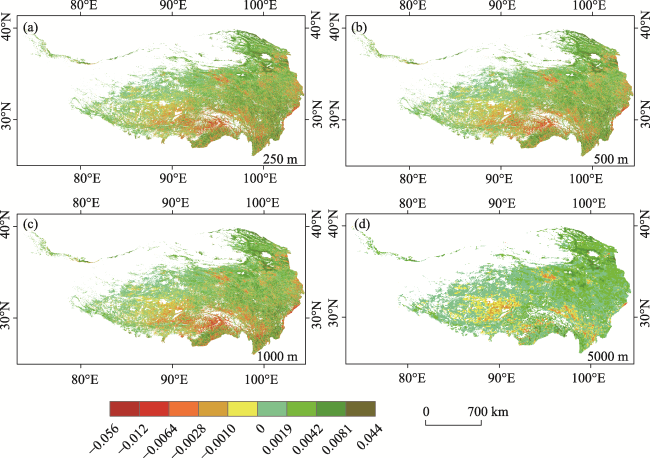
Figure 2 The trend of NDVI interannual trends on spatial scales of 250 m (a), 500 m (b), 1000 m (c), and 5000 m (d) in the Qinghai-Tibet Plateau
By comparing the results among different spatial resolutions (Figures 2a-2d), it can be observed that both the magnitude of trend estimates and their spatial distribution characteristics vary with spatial scales. The magnitudes and spatial distribution characteristics of NDVI trends on relatively fine pixel scales (i.e., 250 m, 500 m, and 1000 m) are similar, showing downward trends in the southern and eastern edges, and strong upward trends in the eastern QTP. But on a larger pixel scale (i.e., 5000 m), the downward trend of the southern QTP significantly decreases. Over the south and east border of QTP, the negative trends in Figures 2a-2c even disappeared or changed to be positive (Figure 2d). Furthermore, the magnitude of the positive trend in the eastern areas on the 5000 m scale (Figure 2d) was generally smaller than other spatial scales (Figures 2a-2c). From these results, it can be concluded that the trend estimates of NDVI show certain dependences on spatial scale, and their discrepancy seems to be related to the spatial scale differences.
To explore the influence mechanism of spatial scale effects on trend estimates, Figure 3 displays the spatial distribution of Diff between different pixel scales. In order to give an intuitive display of the distribution of values of Diff, we also present the histogram of Diff. It can be observed that spatial scale effects showed obvious differences in different regions of QTP (Figure 3). They were weaker and more concentrated in the northwest regions than the southeast regions. Regarding the magnitudes of trend difference, it seems to be dependent on the differences of spatial resolutions. The trend difference of 500 m vs. 250 m was relatively small, with Diff distributed in the range of ‒0.002 to 0.002. This demonstrates that the NDVI trends on the 500 m and 250 m pixel scale are extremely similar. By contrast, the Diff of 1000 m vs. 250 m and 1000 m vs. 500 m were stronger and show larger spatial variability than that of 500 m vs. 250 m. Nevertheless, the Diff of 1000 m vs. 250 m and 1000 m vs. 500 m were similar in both the magnitude and spatial distribution characteristics (Figures 3b and 3c). This indicates that the spatial scale effect may be independent of the fine spatial resolution. This is further confirmed by the results in Figures 3d-3f, where the magnitude and the spatial distribution characteristics of Diff are similar between the 5000 m vs. 250 m, 5000 m vs. 500 m, and 5000 m vs. 1000 m. Therefore, it can be considered that the spatial scale effects are more dependent on the dataset with the coarser spatial resolution. Compared to Figures 3a-3c, the Diff of 5000 m vs. 500 m, 5000 m vs. 250 m, and 5000 m vs. 1000 m are more heterogeneous. And more pixels show relatively larger Diff, indicating that the spatial scale effects are more likely to be significant when the spatial scale difference is large.
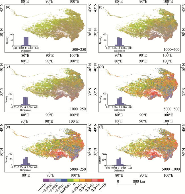
Figure 3 Difference of NDVI interannual trends of 500 m vs. 250 m (a), 1000 m vs. 500 m (b), 1000 m vs. 250 m (c), 5000 m vs. 500 m (d), 5000 m vs. 250 m (e) and 5000 m vs. 1000 m (f) in the Qinghai-Tibet Plateau
From the results above, it can be seen that spatial scale effects widely exist among the datasets with different spatial resolutions, which is consistent with what is generally believed (Hu et al., 1997; Wu et al., 2009). But the magnitude and their spatial distribution characteristics depend on the spatial scale difference. Specifically, the spatial scale effect increases with the spatial scale difference if the dataset with relatively coarser resolutions is not the same, as indicated by the results in Figures 3a, 3c, and 3e. However, as shown in Figures 3d-3f, if the dataset with the relatively coarser resolution is the same, spatial scale effect may not necessarily increase with the spatial scale difference. From Figure 3, it can be seen that the spatial scale effects present strong spatial variations, which may be related to the factors such as topography and vegetation types (Hu et al., 1997; Jiang et al., 2006). To explore the influencing factors on the spatial scale effects, the relationship between spatial scale effects and spatial heterogeneity, vegetation cover types, and topography factors were quantified in the following sections.

4.2 The influencing factors of spatial scale effects

Since the spatial scale effect was mainly affected by the dataset with a coarser spatial resolution, the influencing factors were explored using the results of 500 m vs. 250 m, 1000 m vs. 250 m, and 5000 m vs. 250 m.

4.2.1 Influence of spatial heterogeneity on spatial scale effect

Figure 4 shows the boxplots of Diff for different levels of spatial heterogeneity. It can be seen that Diff do not increase monotonously with spatial heterogeneity. Instead, they even decrease with spatial heterogeneity at certain levels. A typical example can be found at [0.3,0.35], where the Diff of 1000 m vs. 250 m and 5000 m vs. 250 m are smaller than those at [0.25,0.3]. In the case of lower spatial heterogeneity (Diff < 0.25), Diff basically increase monotonously with spatial heterogeneity and the gap of spatial scales. This indicates that the Diff depend more on spatial heterogeneity and spatial scale difference in this circumstance.
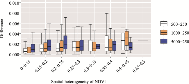
Figure 4 The variation in spatial scale effect with spatial heterogeneity of NDVI
When spatial heterogeneity is larger than 0.25, relatively large fluctuations of Diff appear. This proves that Diff are more influenced by other factors in this situation. Unlike those at [0,0.25], the variation characteristics of Diff with spatial heterogeneity are inconsistent between these three spatial scale effects (i.e., 500 m vs. 250 m, 1000 m vs. 250 m, and 5000 m vs. 250 m). For Diff of 500 m vs. 250 m, the maximum and the width of the boxplot increase with the enhancement of spatial heterogeneity. The Diff of 1000 m vs. 250 m basically increase with spatial heterogeneity at the range of [0,0.25]. Then the magnitude and the width of boxplots decrease with the spatial heterogeneity from [0.25,0.3] to [0.3,0.35] and then increase from [0.35,0.4] to [0.4,0.45]. The Diff of 5000 m vs. 250 m even show more complex variation trends with spatial heterogeneity, which first decrease at [0.3,0.35] and then increase significantly at[0.35,0.4], finally decrease significantly at [0.4,0.45]. These results indicate that larger spatial scale differences may result in spatial scale effects that are more influenced by other factors except for spatial heterogeneity.
Regarding the values of Diff, it shows an increasing trend with the spatial scale difference when spatial heterogeneity is smaller than 0.25. Nevertheless, as spatial heterogeneity becomes larger, this relationship does not hold. For instance, an opposite phenomenon occurs at [0.3, 0.35], where the Diff of 500 m vs. 250 m are the largest but those of 5000 m vs. 250 m are the smallest. This is because there are many factors driving spatial scale effects in the case of large spatial heterogeneity.
Based on the above analysis, we can conclude that in the case of small spatial heterogeneity, spatial scale effects generally increase with the degree of spatial heterogeneity and the spatial scale differences between different datasets. In view of the monotonic change of spatial scale effects with spatial heterogeneity, spatial heterogeneity is considered to play a decisive role in spatial scale effect in this situation. By contrast, in the areas with strong spatial heterogeneity, the dominant role of spatial heterogeneity weakens, and spatial scale effects are jointly affected by other factors. This finding agrees well with Chen et al. (2018) who pointed out that scale effects were not simply caused by spatial heterogeneity. Therefore, other main factors that contribute to spatial scale effects of NDVI trend estimates should be further explored.

4.2.2 Influence of vegetation types on spatial scale effect

The variation of spatial scale effects with vegetation types is displayed in Figure 5. It is obvious that the effect of vegetation types on spatial scale effects is related to the spatial scale difference between different datasets, which is significant for the Diff of 5000 m vs. 250 m and small for the Diff of 500 m vs. 250 m. As can be seen from Figure 5a, the Diff were almost concentrated around 0 for all vegetation types. But the spatial variation of Diff shows relatively large differences among these vegetation types, which is larger for deciduous needleleaf forests and cropland/natural vegetation mosaics, but smaller for open shrubland and grasslands. When it comes to 1000 m vs. 250 m (Figure 5b), Diff become larger, and the spatial variations of Diff are more significant for different vegetation types in this case, indicated by the larger spread of the boxplots.
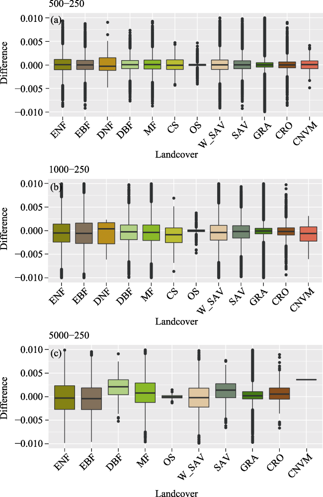
Figure 5 Spatial scale effects as a function of land cover type in the Qinghai-Tibet Plateau: ENF (evergreen needleleaf forests), EBF (evergreen broadleaf forests), DNF (deciduous needleleaf forests), DBF (deciduous broadleaf forests), MF (mixed forests), CS (closed shrublands), OS (open shrubland), W_SAV (woody savannas), SAV (savannas), GRA (grasslands), CRO (croplands), and CNVM (cropland/natural vegetation mosaics)
As shown in Figure 5c, the Diff of 5000 m vs. 250 m show obvious fluctuations with vegetation types. They are small for open shrublands and grasslands, which is basically consistent with the results of 1000 m vs. 250 m and 500 m vs. 250 m. This might be attributed to the weak NDVI heterogeneity of the two vegetation types. By contrast, other vegetation types, such as evergreen needleleaf forests, evergreen broadleaf forests, deciduous broadleaf forests, mixed forests, woody savannas, savannas, and cropland/natural vegetation mosaics showed considerable spatial scale effects. These results indicate that the spatial scale effects should be considered in trend estimates for most of the vegetation types except for open shrublands and grasslands.

4.2.3 Influence of topography on spatial scale effect

In order to explore the relationship between spatial scale effects and topographic factors, the boxplots of Diff at different levels of elevation, slope, aspect, and topographic variability were presented in Figure 6. From Figure 6a, it can be seen that Diff are not changing monotonously with the increase of elevation. Specifically, over the regions lower than 1800 m, the Diff of 500 m vs. 250 m and 1000 m vs. 250 m slightly increase with elevation. Nevertheless, the Diff of 5000 m vs. 250 m do not monotonically increase with the elevations in this region. For the areas higher than 1800 m, the variation characteristics of the Diff between 500 m vs. 250 m and 1000 m vs. 250 m are consistent. They decrease with elevation in the range of [1800 m, 3600 m]. Then a slightly increasing trend appears in the range of [3600 m, 4200 m]. With the further increase of elevation, their Diff decrease with elevation. By contrast, the spatial scale effects of 5000 m vs. 250 m keep decreasing with the increase of elevation in regions higher than 1800 m.
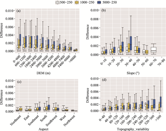
Figure 6 The spatial scale effects as a function of elevation (a), slope (b), aspect (c), and topographic variability (d) in the Qinghai-Tibet Pleteau
The Diff generally increase with the spatial scale differences at different levels of elevation. This can be explained from four aspects: first, the NDVI is not original observations of satellites but is a nonlinear combination of reflectance. Consequently, the NDVI on coarser pixel scales is not equivalent to the averaged values on finer scales; second, the change of NDVI over time is not linear, although trend slopes were regressed linearly as a function of time. Therefore, the trend on a coarse pixel scale is not a simple combination of the trends on finer scales; third, spatial heterogeneity also complicates the relationship of trends between finer and coarser pixel scales; last but not the least, the thresholding effect of specific significance levels also affects the rescaling of trends between different spatial scales. It is noteworthy that these three kinds of spatial scale effects are not significant at regions higher than 4800 m. This occurs because the vegetation at high altitudes is sparse and their interannual variation is weak and homogeneous. Based on the above analysis, it is believed that the spatial scale effects in areas higher than 4800 m are negligible in NDVI trend estimates.
Figure 6b presents the variation of Diff with slope. It is interesting to find that the three kinds of Diff all peaked at [30°, 40°]. They basically increase monotonically with slope from [0°, 10°] to [30°, 40°]. Moreover, Diff present an increasing trend with the spatial scale differences at different levels of slopes in this situation. This indicates that over the areas with slopes less than 40°, the spatial scale effects are jointly determined by spatial scale difference and slopes. Larger spatial scale differences and slopes generally result in larger spatial scale effects in this condition. Nevertheless, this is not the case when the slope is larger than 40°. The Diff of 500 m vs. 250 m at the slope of [40°, 50°] are almost equal to that of [30°, 40°]. But an obvious decrease was found in the Diff of 1000 m vs. 250 m and 5000 m vs. 250 m at the same range of slope. As the slope increases to [50°, 60°], Diff further decrease. And the Diff of 500 m vs. 250 m and 1000 m vs. 250 m are basically equal, after which there are so few pixels that the results may be not representative. These results demonstrate that over the areas with large slopes, spatial scale effects are very complicated and jointly determined by many other factors.
From Figure 6c, it can be seen that the variations of spatial scale effects with aspect are not fixed. Generally, Diff are smaller in the northeast and northwest. This can be attributed to the fact that the NDVI values and their interannual trends are not significant over these areas. By contrast, the areas with the aspect of southeast, south, and southwest, Diff present larger values and a more variable distribution, indicating that spatial scale effects show relatively large spatial variations over the areas with the same aspect. This occurs might because the vegetation types are abundant for the areas with the south aspect, which results in larger spatial heterogeneity of NDVI. The Diff of 5000 m vs. 250 m are generally larger than those of 500 m vs. 250 m and 1000 m vs. 250 m, and it is especially true over the area with the south aspect. From these results, it can be concluded that the spatial scale effects are negligible over the area with the northeast and northwest aspect, but should be taken seriously over the areas with the south aspect.
As shown in Figure 6d, the variation characteristics of Diff with topography variability show a certain dependence on the spatial scale differences. The Diff of 500 m vs. 250 m and 1000 m vs. 250 m do not change monotonously with topography variability. By contrast, the Diff of 5000 m vs. 250 m increase monotonously with topography variability. This occurs partly because larger topography variability is more likely to result in shadows, which causes the larger spatial heterogeneity of NDVI. It is interesting that in the regions with relatively low topography variability [40, 200], the Diff of 5000 m vs. 250 m are lower and more centralized than that of 1000 m vs. 250 m. This may be related to the fact that in the regions with small topography variability, the NDVI variations on the fine-scale are averaged at the coarse pixel scale. Thus, it can be concluded that the topography variability plays a dominant role in the spatial scale effects of 5000 m vs. 250 m, which can be negligible in the case of small topography variability, and vice versa. The spatial scale effects of 500 m vs. 250 m and 1000 m vs. 250 m are jointly determined by many other factors.

4.3 Temporal scale effect on trend estimates

The temporal scale effect of trend estimates based on satellite data has been gradually realized as well (Liu et al., 2017; Wu et al., 2021). Here, we present the trend estimate of GPP using the dataset with different temporal scales (Figure 7). It can be seen that the trends of GPP are not completely consistent among different temporal scales. For western QTP, although the overall trend of different temporal scales is weak, the negative trend areas in Figure 7c is larger than that in Figures 7a and 7b. For eastern QTP, the positive trend of GPP presents similar spatial distribution characteristics between 8-day and annual scales (Figures 7a and 7c). The trend in the east-central of QTP is located in the range of 0.01 to 0.016 g Cm‒2 yr‒1. By contrast, in the eastern and southern edges of QTP, the GPP variation trend is large, with values ranging from 0.25 to 0.45 g Cm‒2 yr‒1. Different from the positive trend, the number of pixels with negative trends on the annual scale is much larger than those on the 8-day scale. This confirms that larger areas present negative trends on the annual scale. Compared to the trends on the 8-day and annual scale, the negative trends of QTP seem to be weaker on the monthly scale and even change to positive on the southern edge of QTP.
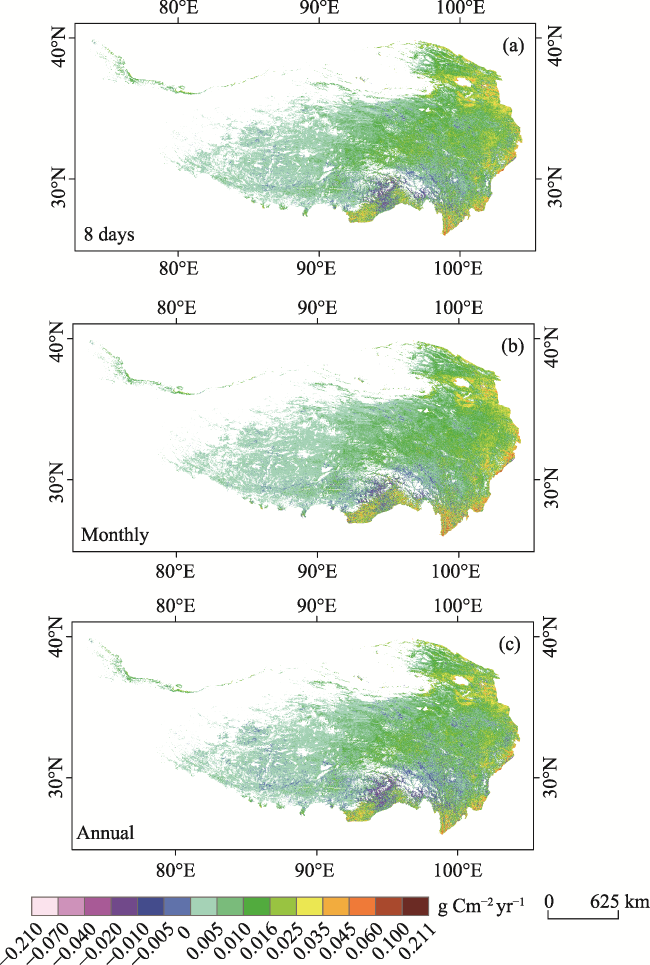
Figure 7 The trend of GPP interannual trends on temporal scales of 8-day (a), monthly (b), and annual (c) in the Qinghai-Tibet Plateau
To explore the magnitude of the differences caused by different temporal scales, we present the difference of the trend estimates between different temporal scales in Figure 8. Overall, the spatial pattern of the temporal scale effects was highly heterogeneous, with relatively strong differences in the southeast and weak differences in the northwest. However, the magnitude of difference shows dependence on the temporal scale difference. Specifically, the temporal scale effect of annual vs. monthly was the strongest. It is unexpected that the temporal scale effects of annual vs. 8-day are the weakest. This phenomenon indicates that the GPP interannual trend estimated with the annual scale dataset was similar to those estimated with the 8-day dataset. But they show obvious differences from those estimated with monthly scale datasets. This can be attributed to the fact that for the annual scale, the time step is large and some short-term changes are averaged out. Although the 8-day temporal scale could capture more variations of GPP, it also involves a lot of noise, which obscures some change details to a certain degree. By contrast, the monthly temporal scale contains more vegetation phenological information than the 8-day and annual temporal scale.
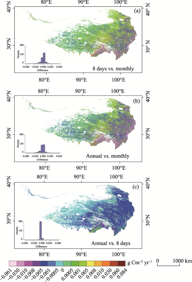
Figure 8 Difference of GPP interannual trends of 8 days vs. monthly (a), annual vs. monthly (b) and annual vs. 8 days (c) in the Qinghai-Tibet Plateau

4.4 The influencing factors of temporal scale effect

The influence of vegetation types and topography on temporal scale effect of the GPP trend was explored here. However, the influence of spatial heterogeneity of GPP was not focused on due to the lack of high-resolution GPP datasets.

4.4.1 Influence of vegetation types on temporal scale effect

The change of temporal scale effect with vegetation types is shown in Figure 9. Similar to the spatial scale effect, the temporal scale effect of different vegetation types is influenced by the temporal scale difference of the datasets, which is significant for the Diff of day vs. month and annual vs. month but small for the Diff of annual vs. day. From Figures 9a and 9b, the Diff fluctuations with vegetation types, which is small for open shrubland and grasslands but prominent for deciduous broadleaf forests and cropland/natural vegetation mosaics. The reason for this phenomenon might be that the spatial distribution of open shrubland and grasslands is relatively concentrated, and their spatial heterogeneities are weak. From Figure 9c, although the Diff between annual vs. day are small, it still fluctuate by vegetation types. Comparing different vegetation types, we found that the temporal scale effects of open shrubland and grasslands are independent of temporal scale differences. Therefore, the influence of the scale effect can be ignored when estimating trends of open shrubland and grassland with different temporal resolution products.
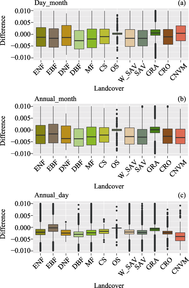
Figure 9 Temporal scale effects as a function of land cover type in the Qinghai-Tibet Plateau: ENF (evergreen needleleaf forests), EBF (evergreen broadleaf forests), DNF (deciduous needleleaf forests), DBF (deciduous broadleaf forests), MF (mixed forests), CS (closed shrublands), OS (open shrubland), W_SAV (woody savannas), SAV (savannas), GRA (grasslands), CRO (croplands), and CNVM (cropland/natural vegetation mosaics)

4.4.2 Influence of topography on temporal scale effect

The relationship between temporal scale effect and topographic factors (elevation, slope, aspect, and topographic variability) is shown in Figure 10. From Figure 10a, it was seen that Diff do not vary monotonically with elevation. Specifically, for the regions lower than 1800 m, Diff of daily vs. annual and annual vs. monthly increase monotonically with elevation, and the maximum values of these two kinds of Diff occur in the range of [1200 m, 1800 m]. Nevertheless, the Diff of annual vs. daily fluctuate slightly with the change of altitude, and its maximum appear in the interval [1800 m, 2400 m]. Similar to spatial scale effect of 5000 m vs. 250 m (Figure 6a), for the regions higher than 1800 m, the three kinds of Diff all decrease with elevation. It is noteworthy that Diff are smaller in the regions with an elevation higher than 4800 m, where temporal scale effect can be ignored.
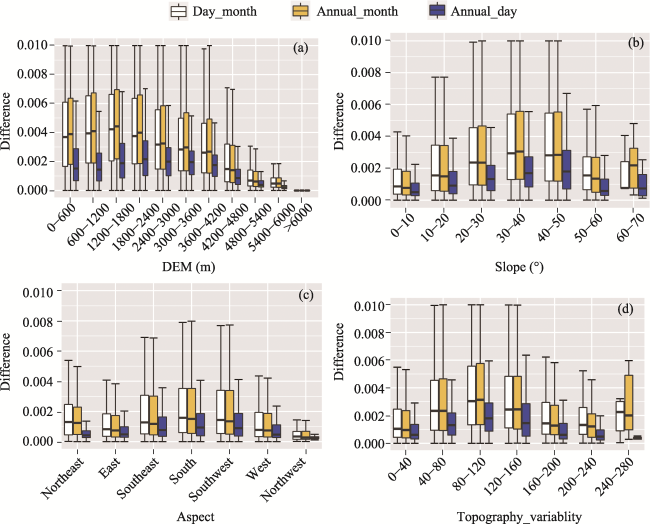
Figure 10 The temporal scale effects as a function of elevation (a), slope (b), aspect (c), and topographic variability (d) in the Qinghai-Tibet Plateau
Figure 10b shows the variation of temporal scale effect with slope. For the area with a slope lower than 50°, the three types of Diff monotonically increase with slope and peaked in the interval of [40°, 50°], indicating the decisive role of slope on temporal scale effects in this situation. Furthermore, it can be found that Diff also vary with temporal scale difference at each specific level of slope. This indicates that temporal scale effect is jointly affected by the temporal scale difference and slope in this situation. Compared with Figure 6b, it was found that in the regions with a slope lower than 40°, the variation pattern of spatial scale effect with slope is consistent with that of temporal scale effect. This phenomenon suggests that for the middle and small slope regions, the slope has a strong influence on the spatiotemporal scale effect, and this influence is independent of vegetation indices and satellite datasets. For the regions with the slope interval of [50°, 60°], the three kinds of Diff decrease with slope. This can be explained by the fact that the temporal scale effect is jointly influenced by many other factors.
From Figure 10c, it can be seen that the Diff in the south, southeast, and southwest were relatively larger and scattered, followed by the east and west, and the Diff in the northwest are the weakest and concentrated, which coincide with the distribution pattern of the spatial scale effect. This indicates that the spatiotemporal scale effect shows a strong dependence on the aspect. However, an unexpected situation occurred in the northeast, where the Diff of daily vs. monthly and annual vs. monthly are higher than that of the east and west. This is inconsistent with the case of the spatial scale effect, which is reasonable since the numbers of vegetation pixels in the northeast are limited. Hence, the results are not representative. Based on these results, it can be concluded that the temporal scale effect can be neglected over the northwest, but should be fully considered over the regions with the south aspect.
Figure 10d shows the variation of temporal scale effect with topography variability. The variation patterns of these three kinds of Diff were basically consistent. Specifically, Diff first increase monotonically with topography variability within the range of [0, 120]. Then they decrease with the topography variability from 120 to 200. Finally, a slight fluctuation occurs at the interval of [200, 280].
Based on the results in sections 4.2.3 and 4.4.2, it can be concluded that the spatiotemporal scale effect is jointly affected by the difference in spatiotemporal resolution and topography changes. Specifically, for the areas with moderate elevation and relatively small slope, spatiotemporal scale effect is mainly dominated by altitude and slope. For the extremely high elevation (> 4800 m), spatiotemporal scale effect is relatively weak due to the sparse vegetation coverage. Therefore, in this case, scale effect can be neglected. For the south aspect regions, spatiotemporal scale effects are the largest due to strong vegetation heterogeneity. By contrast, in the regions with the northwest aspect, it is small enough to be neglected. In addition, the influence of topography variability on spatiotemporal scale effect is also dependent on the scale difference. For instance, topography variability shows a larger influence on the spatial scale effect of 5000 m vs. 250 m than those of 1000 m vs. 250 m and 500 m vs. 250 m. For the regions with low topography variability, spatial scale effect can be ignored. In terms of temporal scale effect, it can be ignored for annual vs. daily, but should be fully considered for daily vs. monthly and annual vs. monthly for the areas with extremely low and high topography variability.
In summary, over the regions with sparse vegetation and low topography variability, the spatiotemporal scale effect on trend estimation of vegetation change can be neglected. Moreover, it was found that the temporal and spatial scale effects of different vegetation indicators present the same variation pattern with topography and and vegetation types. This demonstartes that the topography and vegetation types should be an important consideration in illustrating the trend estimates of vegetation change with different spatiotemporal scales.

5 Conclusions

The NDVI and GPP changing trends are critical to understanding the variation of vegetation and its photosynthetic carbon assimilation ability. Satellite products with different spatiotemporal resolutions have been widely used to detect interannual trends at global or regional scales. Nevertheless, the uncertainties of trend estimates caused by spatiotemporal scale effects have received relatively little attention. This study made a quantitative and systematic analysis of the spatiotemporal scale effects on trend estimates based on satellite datasets. In addition, the influencing factors (i.e., spatial heterogeneity, topography, and vegetation types) related to the spatiotemporal scale effect have been investigated as well.
It was found that spatial scale effects show more dependence on the dataset with the coarser spatial resolution. Once the coarse resolution was fixed, they are not necessarily positively related to the spatial scale gap between different datasets. Hence, the coarse-resolution satellite data should be selected with caution in detecting the trend of vegetation change. Different from spatial scale effect, temporal scale effect is mianly affected by the difference of temporal scales. The temporal scale effects between daily and yearly scales are negligible. However, the trend estimates on the monthly scale show large difference than those of daily and yearly scales. Hence, the trend estimates based on daily/yearly scale data and monthly scale data are not comparable. The spatial scale effect does not always positive response to spatial heterogeneity. But they can be ignored for the regions with low spatial heterogeneity. Spatial scale effect is also influenced by the spatial scale gap and the variation of topography. For the regions with sparse vegetation (i.e., extremely high elevation and the aspect of northeast, west, and northeast) and low topography variability, spatial scale effect on trend estimates of vegetation change can be ignored. Regarding the influence of vegetation types, the spatial scale effect of grassland and open shrubland is small and stable, and thus can be neglected when detecting the trend of vegetation change. It is interesting to find that the variation of temporal scale effect with topography and vegetation types is highly similar to that of the spatial scale effect, indicating that the topography and vegetation types should be an important consideration in illustrating the trend estimates of vegetation change with different spatiotemporal scales.
Although the spatiotemporal scale effects are merely explored over QTP using MODIS NDVI and GPP products, the findings and conclusion can be transferable to other regions to a certain degree due to the wide range of conditions (e.g., elevation, topography, and land cover) of QTP. Nevertheless, it is noteworthy that the trend estimate depends strongly on the trend detection methods. Thus, it is still an open issue whether the linear regression is sufficient to model the spatiotemporal scale effects in NDVI and GPP trend estimates. Despite this limitation, the study still deepens the consciousness and understanding of the detected trends which were not related to actual changes of the earth but caused by spatiotemporal scales of satellite data themselves. Furthermore, it provides reasonable suggestions for choosing suitable satellite products for trend estimates in different conditions, which is the first step towards a more robust trend estimate based on satellite datasets.

Data availability statement

MODIS Version 6 NDVI products, including MOD13Q1, MOD13A1, and MOD13A2, were obtained from the Google Earth Engine (https://developers.google.com/earth-engine/datasets/catalog/modis). MODIS GPP product (i.e., MOD17A2H v006) , the land cover types products (i.e., MCD12Q1 V6) , and the DEM products (SRTM) were also obtained from the Google Earth Engine via the link https://developers.google.com/earthengine/datasets/catalog/MODIS_006_MOD17A2H, https://developers.google.com/earth-engine/datasets/catalog/ MODIS_006_MCD12Q1, and https://developers.google.com/earth-engine/datasets/catalog/ CGIAR_SRTM90_V4, respectively. MOD13C1 were downloaded from the Land Processes Distributed Active Arcchive Center (LP DAAC) via the link https://lpdaac.usgs.gov/products/mod13c1v006/.
[1]
Alcaraz-Segura D O, Chuvieco E, Epstein H E et al., 2010. Debating the greening vs. browning of the North American boreal forest: Differences between satellite datasets. Global Change Biology, 16(2): 760-770.

DOI

[2]
Anderson K, Fawcett D, Cugulliere A et al., 2020. Vegetation expansion in the subnival Hindu Kush Himalaya. Global Change Biology, 26(3): 1608-1625.

DOI PMID

[3]
Beck H E, McVicar T R, van Dijk A I et al., 2011. Global evaluation of four AVHRR-NDVI data sets: Intercomparison and assessment against Landsat imagery. Remote Sensing of Environment, 115(10): 2547-2563.

DOI

[4]
Chen K, Li S, Zhou Q et al., 2007. Multi-scale study on climate change for recent 50 years in Dari county in the source regions of the Yangtze and Yellow rivers. Geographical Research, 26(3): 526. (in Chinese)

DOI

[5]
Chen X, Wang D, Chen J et al., 2018. The mixed pixel effect in land surface phenology: A simulation study. Remote Sensing of Environment, 211: 338-344.

DOI

[6]
Cheng C, Li B, Ma T, 2003. The application of very high resolution satellite image in urban vegetation cover investigation: A case study of Xiamen City. Journal of Geographical Sciences, 13(2): 265-270.

DOI

[7]
De Beurs K M, Wright C K, Henebry G M, 2009. Dual scale trend analysis for evaluating climatic and anthropogenic effects on the vegetated land surface in Russia and Kazakhstan. Environmental Research Letters, 4(4): 045012.

DOI

[8]
Fagua J C, Ramsey R D, 2019. Comparing the accuracy of MODIS data products for vegetation detection between two environmentally dissimilar ecoregions: The Chocó-Darien of South America and the Great Basin of North America. GIScience & Remote Sensing, 56(7): 1046-1064.

[9]
Fensholt R, Proud S R, 2012. Evaluation of earth observation based global long term vegetation trends: Comparing GIMMS and MODIS global NDVI time series. Remote Sensing of Environment, 119: 131-147.

DOI

[10]
Fensholt R, Rasmussen K, Nielsen T T et al., 2009. Evaluation of earth observation based long term vegetation trends: Intercomparing NDVI time series trend analysis consistency of Sahel from AVHRR GIMMS, Terra MODIS and SPOT VGT data. Remote Sensing of Environment, 113(9): 1886-1898.

DOI

[11]
Ghazaryan G, 2015. Analysis of temporal and spatial variations of forest. A case of study in northeastern Armenia 9[D].

[12]
Gorelick N, Hancher M, Dixon M et al., 2017. Remote Sensing of Environment, 202: 18-27.

DOI

[13]
Hu Z, Islam S, 1997. A framework for analyzing and designing scale invariant remote sensing algorithms. IEEE Transactions on Geoscience and Remote Sensing, 35(3): 747-755.

DOI

[14]
Ichii K, Kawabata A, Yamaguchi Y, 2002. Global correlation analysis for NDVI and climatic variables and NDVI trends: 1982-1990. International Journal of Remote Sensing, 23(18): 3873-3878.

DOI

[15]
Jiang Z, Huete A R, Chen J et al., 2006. Analysis of NDVI and scaled difference vegetation index retrievals of vegetation fraction. Remote Sensing of Environment, 101(3): 366-378.

DOI

[16]
Li P, Hu Z, Liu Y, 2020. Shift in the trend of browning in southwestern Tibetan Plateau in the past two decades. Agricultural and Forest Meteorology, 287: 107950.

DOI

[17]
Liang D, Zuo Y, Huang L et al., 2015. Evaluation of the consistency of MODIS Land Cover Product (MCD12Q1) based on Chinese 30 m GlobeLand30 datasets: A case study in Anhui province, China. ISPRS International Journal of Geo-Information, 4(4): 2519-2541.

DOI

[18]
Liu L, Liu L, Liang L et al., 2014. Effects of elevation on spring phenological sensitivity to temperature in Tibetan Plateau grasslands. Chinese Science Bulletin, 59(34): 4856-4863.

DOI

[19]
Liu S, Cheng F, Dong S et al., 2017. Spatiotemporal dynamics of grassland aboveground biomass on the Qinghai-Tibet Plateau based on validated MODIS NDVI. Scientific Reports, 7(1): 1-0.

DOI

[20]
Liu W, Chen S, Qin X et al., 2012. Storage, patterns, and control of soil organic carbon and nitrogen in the northeastern margin of the Qinghai-Tibetan Plateau. Environmental Research Letters, 7(3): 035401.

DOI

[21]
Liu X, Zhang J, Zhu X et al., 2014. Spatiotemporal changes in vegetation coverage and its driving factors in the Three-River Headwaters Region during 2000-2011. Journal of Geographical Sciences, 24(2): 288-302.

DOI

[22]
Monteith J L, 1972. Solar radiation and productivity in tropical ecosystems. Journal of Applied Ecology, 9(3): 747-766.

DOI

[23]
Mu S, Yang H, Li J et al., 2013. Spatio-temporal dynamics of vegetation coverage and its relationship with climate factors in Inner Mongolia, China. Journal of Geographical Sciences, 23(2): 231-246.

DOI

[24]
Tian F, Fensholt R, Verbesselt J et al., 2015. Evaluating temporal consistency of long-term global NDVI datasets for trend analysis. Remote Sensing of Environment, 163: 326-340.

DOI

[25]
Wen J, You D, Han Y et al., 2022. Estimating surface BRDF/Albedo over rugged terrain using an Extended Multisensor Combined BRDF Inversion (EMCBI) Model. IEEE Geoscience and Remote Sensing Letters, 19: 1-5.

[26]
Wu H, Li Z L, 2009. Scale issues in remote sensing: A review on analysis, processing and modeling. Sensors, 9(3): 1768-1793.

DOI PMID

[27]
Wu X, Ma D, Wang J et al., 2021. Temporal scale effects on trend estimates for solar radiation, thermal and snow conditions, and their feedbacks: The case from China. Theoretical and Applied Climatology, 146(3): 869-882.

DOI

[28]
Xia J, Niu S, Ciais P et al., 2015. Joint control of terrestrial gross primary productivity by plant phenology and physiology. Proceedings of the National Academy of Sciences, 112(9): 2788-2793.

DOI

[29]
Yu Z, Wang J, Liu S et al., 2013. Inconsistent NDVI trends from AVHRR, MODIS, and SPOT sensors in the Tibetan Plateau. In: 2013 Second International Conference on Agro-Geoinformatics (Agro-Geoinformatics), 97-101.

[30]
Yuan Q, Yuan Q, Ren P, 2021. Coupled effect of climate change and human activities on th restoration/degradation of the Qinghai-Tibet Plateau grassland. Journal of Geographical Sciences, 31(9): 1299-1327.

DOI

[31]
Zhang Y, Xu G, Li P et al., 2019. Vegetation change and its relationship with climate factors and elevation on the Tibetan Plateau. International Journal of Environmental Research and Public Health, 16(23): 4709.

DOI

[32]
Zhao H, Liu S, Dong S et al., 2015. Analysis of vegetation change associated with human disturbance using MODIS data on the rangelands of the Qinghai-Tibet Plateau. The Rangeland Journal, 37(1): 77-87.

DOI

[33]
Zhao J, Chen X, Bao A et al., 2009. A method for choice of optimum scale on land use monitoring in Tarim River Basin. Journal of Geographical Sciences, 19(3): 340-350.

DOI

[34]
Zhu X, Pei Y, Zheng Z et al., 2018. Underestimates of grassland gross primary production in MODIS standard products. Remote Sensing, 10(11): 1771.

DOI

Outlines

/