
Journal of Geographical Sciences >
Assessment of the fraction of bed load concentration towards the sediment transport of a monsoon-dominated river basin of Eastern India
Received date: 2022-06-13
Accepted date: 2023-01-03
Online published: 2023-05-11
Supported by
Ministry of Water Resources, Government of India(28/1/2016-R&D/228-245)
Given the challenges of re-creating complex bed load (BL) transport processes in rivers, models are preferred over gathering and examining field data. The highlight of the present research is to develop an approach to determine the ungauged bed load concentration (BLCu) utilizing the measured suspended sediment concentration (SSC) and hydraulic variables of the last four decades for the Mahanadi River Basin. This technique employs shear stress and SSC equations for turbulent open channel flow. Besides, the predicted BLCu is correlated with SSC using a power relation to estimate BLCu on the river and tributaries. Eventually, different BL functions (BLF) efficiency is assessed across stations. The model predicted BLCu is comparable with the published data for sandy rivers and falls within ± 20%. Outliers in hydraulic and sedimentological statistics significantly influence estimating the BL fraction apart from higher relative ratios and catchment geology. The constants of power functions are physically linked to sediment transport configuration, mechanism, and inflow to the stream. The stream power-based BLF best predicts the BL transport, followed by shear stress and unit discharge approaches. The disparity in the estimation of BLCu results from station-specific physical factors, sampling data dispersion, and associated uncertainties.
KAR Rohan , SARKAR Arindam . Assessment of the fraction of bed load concentration towards the sediment transport of a monsoon-dominated river basin of Eastern India[J]. Journal of Geographical Sciences, 2023 , 33(5) : 1023 -1054 . DOI: 10.1007/s11442-023-2118-6
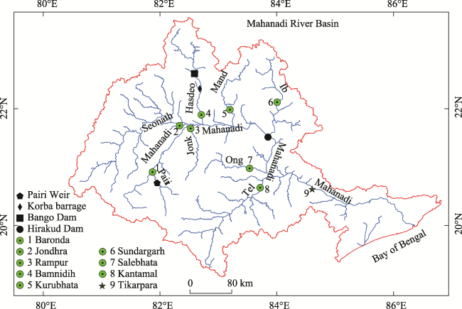
Figure 1 A map of the Mahanadi River Basin showing hydrological stations |
Table 1 Summary of hydrological stations considered in the present study |
| Gauging stations | Latitude (o) | Longitude (o) | Data interval | Altitude (m.a.s.l) | Drainage area (km2) | Tributary/Sub-tributary |
|---|---|---|---|---|---|---|
| Baronda | 20.91 | 81.89 | 1980-2017 | 283 | 3225 | Pairi |
| Jondhra | 21.73 | 82.35 | 1981-2017 | 219 | 29,645 | Seonath |
| Rampur | 21.65 | 82.52 | 1977-2017 | 219 | 2920 | Jonk |
| Bamnidih | 21.90 | 82.72 | 1973-2017 | 223 | 9730 | Hasdeo |
| Kurubhata | 21.99 | 83.20 | 1980-2017 | 215 | 4625 | Mand |
| Sundargarh | 22.12 | 84.01 | 1980-2017 | 214 | 5870 | Ib |
| Salebhata | 20.98 | 83.54 | 1973-2017 | 130 | 4650 | Ong |
| Kantamal | 20.65 | 83.73 | 1977-2017 | 118 | 19,600 | Tel |
| Tikarpara | 22.63 | 84.62 | 1973-2017 | 50 | 124,450 | Mahanadi |
Note: m.a.s.l = m above sea level |
Table 2 Particulars of percentage classification of dominant soil classes across stations of the study |
| Hydrological stations | Percentage sand, Psand (%) | Percentage silt, Psilt (%) | Percentage clay, Pclay (%) |
|---|---|---|---|
| Baronda | 32.400 | 19.900 | 47.700 |
| Jondhra | 64.400 | 13.600 | 22.100 |
| Rampur | 64.400 | 13.600 | 22.100 |
| Bamnidih | 64.400 | 13.600 | 22.100 |
| Kurubhata | 23.300 | 36.700 | 40.000 |
| Sundargarh | 61.100 | 15.300 | 23.700 |
| Salebhata | 59.150 | 20.300 | 20.550 |
| Kantamal | 32.000 | 25.100 | 43.000 |
| Tikarpara | 56.400 | 15.300 | 28.400 |
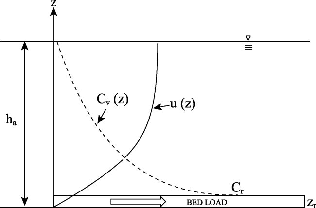
Figure 2 Schematic of the distribution of the vertical velocity and suspended sediment concentration |
Table 3 Correlation between Re and$\hat{p}$ |
| Re | ≤0.1 | 0.2 | 0.5 | 1.0 | 2.0 | 5.0 | 10.0 | 20.0 | 50.0 | 100.0 | 200.0 | ≥500.0 |
|---|---|---|---|---|---|---|---|---|---|---|---|---|
| $\hat{p}$ | 4.91 | 4.89 | 4.83 | 4.78 | 4.69 | 4.51 | 4.25 | 3.89 | 3.33 | 2.92 | 2.58 | 2.25 |
Table 4 Correlation between d65/δ° and λ |
| d65/δ° | 0.2 | 0.3 | 0.5 | 0.7 | 1.0 | 2.0 | 4.0 | 6.0 | 10.0 |
|---|---|---|---|---|---|---|---|---|---|
| λ | 0.7 | 1.0 | 1.38 | 1.56 | 1.61 | 1.38 | 1.10 | 1.03 | 1.0 |
Table 5 Fraction of the ungauged bed load concentration as per Maddock and Borlanda (1950) and Lane and Borlandb (1951) |
| Suspended sediment concentration (ppm) | Bed material class | Texture of suspended sediment | % BL relative to TLa | % BL relative to SLb |
|---|---|---|---|---|
| < 1000 | Sand | Similar to bed material | Up to 50 | 25-150 |
| < 1000 | Gravel, rock or consolidated clay | Small amount of sand | 5 | 5-12 |
| 1000-7500 | Sand | Similar to bed material | 10-20 | 10-35 |
| 1000-7500 | Gravel, rock or consolidated clay | 25% sand or less | 5-10 | 5-12 |
| > 7500 | Sand | Similar to bed material | 10-20 | 5-15 |
| > 7500 | Gravel, rock or consolidated clay | 25% sand or less | 2-8 | 2-8 |
Note: BL: Bed load, SL: Suspended load, TL: Total load |
Table 6 Fraction of the ungauged bed load concentration as per Williams and Rosgen (1989) in sandy bed rivers |
| Average concentration of SSC (g/l) (× 10-3) | 1 | 3 | 5.2 | 10.9 | 20.7 | 40.8 | 80.4 | 160.6 |
|---|---|---|---|---|---|---|---|---|
| (Average ± SD) of BL relative to TL (%) | 99.7±0 | 99.2±0.80 | 84±19 | 80±21 | 70±16 | 57±26 | 52±30 | 36±31 |
| Average concentration of SSC (g/l) (× 10-3) | 317.1 | 631.1 | 1131 | 2395 | 4918 | 8006 | 23450 | |
| (Average ± SD) of BL relative to TL (%) | 27±25 | 11±9 | 9±7 | 10±11 | 13±8.20 | 8±6.30 | 1±0.04 |
Note: BL: Bed load, TL: Total load, SD: Standard deviation |
Table 7 Bed load functions incorporated in the present study |
| Bed load functions (Approaches involved) | Functional equations | Parameters involved | |
|---|---|---|---|
| Shields, 1936 (Shear stress) | $\begin{align} & \frac{{{q}_{b}}{{\gamma }_{s}}}{q\gamma {{S}_{a}}}=10\frac{\tau -{{\tau }_{c}}}{\left( {{\gamma }_{s}}-\gamma \right){{d}_{50}}} \\ & \tau =\gamma {{h}_{a}}{{S}_{a}} \\ & {{\tau }_{c}}={{\theta }_{c}}\left( s-1 \right)\gamma {{d}_{50}} \\ & {{\theta }_{c}}=0.1414S_{*}^{-0.23},{{S}_{*}}\le 6.61 \\ & {{\theta }_{c}}=\frac{{{\left[ 1+{{\left( 0.0223{{S}_{*}} \right)}^{2.84}} \right]}^{0.35}}}{3.09S_{*}^{0.68}},6.61<{{S}_{*}}<282.84 \\ & {{\theta }_{c}}=0.045,{{S}_{*}}\ge 282.84 \\ & {{S}_{*}}=\frac{{{d}_{50}}\sqrt{\left( s-1 \right)g{{d}_{50}}}}{\upsilon } \\ \end{align}$ | qb = bedload transport rate [(m3/s)/m] q = unit flow discharge [(m3/s)/m] γs = specific weight of sediment [KN/m3] γ = specific weight of water [KN/m3] Sa = average longitudinal bed slope [m/m] τ = bed shear stress [KN/m2] τc = critical shear stress [KN/m2] d50 = particle size [mm] ha = mean flow depth [m] θc = critical shields stress given by Cao et al. (2006) s = specific gravity of sediment = 2.65 ν = kinematic viscosity of water [m2/s] g = acceleration due to gravity = 9.81 [m/s2] | |
| Schoklitsch, 1962 (Unit flow discharge) | $\begin{align} & {{q}_{c}}=\frac{1.944\times {{10}^{-5}}}{{{S}_{a}}^{{}^{4}/{}_{3}}} \\ & {{q}_{b}}=\frac{7000\times S_{a}^{1.5}\times \left( {{q}_{w}}-{{q}_{c}} \right)}{d_{50}^{0.5}} \\ \end{align}$ | qb = bedload transport rate [(kg/s)/m] qw = unit flow discharge [(m3/s)/m] qc = unit critical flow discharge [(m3/s)/m] d50 = particle size (mm) Sa = average longitudinal bed slope (m/m) | |
| Bagnold, 1980 (Stream power) | $\begin{align} & \frac{{{i}_{b}}}{i_{b}^{*}}=\frac{{{\left( W-{{W}_{0}} \right)}^{1.5}}}{{{\left( W-{{W}_{0}} \right)}^{*}}}{{\left( \frac{Y}{{{Y}^{*}}} \right)}^{-2/3}}{{\left( \frac{D}{{{D}^{*}}} \right)}^{-0.5}} \\ & {{W}_{0}}=290\times {{D}^{1.5}}\log \left( \frac{12Y}{D} \right) \\ \end{align}$ | ib = bedload transport rate [(kg/s)/m] ib* = 0.1 [(kg/s)/m] W = stream power [(kg/s)/m] W0 = threshold stream power [(kg/s)/m] Y = mean flow depth (m) D = d50 = particle size (m) (W-W0) * = 0.5 [(kg/s)/m] Y* = 0.1 (m) D* = 1.1×10⁻³ (m) | |
| Roorkee (Misri et al., 1984; Samaga et al., 1986) (Shear stress) | $\begin{align} & {{\phi }_{b}}=4.6\times {{10}^{7}}{{{{\tau }'}}_{*}}^{8},{{{{\tau }'}}_{*}}\le 0.065 \\ & {{\phi }_{b}}=\frac{8.5{{{{\tau }'}}_{*}}^{1.8}}{{{\left( 1+5.95\times {{10}^{-6}}{{{{\tau }'}}_{*}}^{-4.7} \right)}^{1.43}}},{{{{\tau }'}}_{*}}>0.065. \\ & {{{{\tau }'}}_{*}}=\frac{{{R}_{b}}{{S}_{a}}}{(s-1){{d}_{50}}},{{R}_{b}}={{\left( \frac{{{v}_{a}}}{{{K}_{b}}\sqrt{{{S}_{a}}}} \right)}^{1.5}} \\ & {{K}_{b}}=\frac{K{{K}_{w}}{{(FW)}^{2/3}}}{{{\left[ (FW)K_{w}^{1.5}+2{{h}_{a}}\left( K_{w}^{1.5}-{{K}^{1.5}} \right) \right]}^{2/3}}} \\ & K=\frac{25.8}{{{\left( 2{{d}_{90}} \right)}^{1/6}}} \\ & {{K}_{w}}=\frac{1}{0.009} \\ & {{\phi }_{b}}=\frac{{{q}_{b}}}{{{d}_{50}}\sqrt{\left( s-1 \right)g{{d}_{50}}}} \\ \end{align}$ | ϕb = non-dimensional bed load transport rate ${{{\tau }''}_{*}}$= non-dimensional grain shear stress Rb = hydraulic radius of bed region (m) Sa = average longitudinal bed slope (m/m) s = specific gravity of sediment = 2.65 d50 = particle size (m) va = average flow velocity (m/s) Kb = resistance coefficient of bed K = general resistance coefficient Kw = resistance coefficient of channel walls FW = flow width (m) d90 = particle size at which 90% of the sediment is finer by weight (m) qb = unit bedload transport [(m3/s)/m] | |
| Julien, 2002 (Shear stress) | $\begin{align} & {{q}_{b}}=18\sqrt{g}d_{50}^{1.5}\tau _{*}^{2} \\ & {{\tau }_{*}}=\frac{{{h}_{a}}{{S}_{a}}}{(s-1){{d}_{50}}} \\ \end{align}$ | qb = unit bedload transport [(m3/s)/m] g = 9.81 m/s2 d50 = particle size (m) τ* = Shields parameter ha = mean flow depth (m) Sa = average longitudinal bed slope (m/m) s = specific gravity of sediment = 2.65 | |
| Huang, 2010 [Reformulated Meyer-Peter and Muller, 1948] (Shear stress) | $\begin{align} & \phi =6{{\left( \eta \tau _{b}^{*}-0.047 \right)}^{5/3}} \\ & \eta =0.9997{{\left( \frac{{{K}_{b}}}{{{K}_{s}}} \right)}^{1.1981}} \\ & {{K}_{b}}=\frac{K{{K}_{w}}{{(FW)}^{2/3}}}{{{\left[ (FW)K_{w}^{1.5}+2{{h}_{a}}\left( K_{w}^{1.5}-{{K}^{1.5}} \right) \right]}^{2/3}}} \\ & {{K}_{s}}=\frac{25.8}{{{\left( 2{{d}_{90}} \right)}^{1/6}}} \\ & {{K}_{w}}=\frac{1}{0.009} \\ & \tau _{b}^{*}=\frac{{{R}_{b}}{{S}_{a}}}{(s-1){{d}_{50}}},{{R}_{b}}={{\left( \frac{{{v}_{a}}}{{{K}_{b}}\sqrt{{{S}_{a}}}} \right)}^{1.5}} \\ \end{align}$ | ϕb = non-dimensional bed load transport rate η = bedform correction τb* = non-dimensional bed shear stress Rb = hydraulic radius of bed region (m) Sa = average longitudinal bed slope (m/m) s = specific gravity of sediment = 2.65 d50 = particle size (m) va = average flow velocity (m/s) Kb = resistance coefficient of bed Ks = general resistance coefficient for skin friction Kw = resistance coefficient of channel walls FW = flow width (m) d90 = particle size at which 90% of the sediment is finer by weight (m) qb = unit bedload transport [(m3/s)/m] | |
| Recking, 2013 (Shear stress) | $\begin{align} & \phi =\frac{14\tau _{84}^{{{*}^{2.5}}}}{1+{{\left( \tau _{m}^{*}/\tau _{84}^{*} \right)}^{4}}} \\ & \tau _{m}^{*}=0.045\text{ for sand} \\ & \tau _{84}^{*}=\frac{{{S}_{a}}}{(s-1){{d}_{84}}\times \left[ \left( 2/FW \right)+74{{p}^{2.6}}{{\left( g{{S}_{a}} \right)}^{p}}{{q}^{-2p}}d_{84}^{3p-1} \right]} \\ & \text{where }p=0.23\text{ when }\frac{q}{\sqrt{g{{S}_{a}}d_{84}^{3}}}<100\text{ and }p=0.3\text{ otherwise} \\ & q=Q/FW \\ \end{align}$ | ϕ = Einstein non-dimensional bed load transport rate $\phi =\frac{{{q}_{b}}}{\sqrt{\left( s-1 \right)gd_{84}^{3}}}$ qb = unit bedload transport [(m3/s)/m] g = 9.81 m/s2 d84 = particle size at which 84% of the sediment is finer by weight (m) τ84* = Shields stress for d84 τm* = mobility shear stress Sa = average longitudinal bed slope (m/m) s = specific gravity of sediment = 2.65 FW = flow width (m) | |
Table 8 Characteristics of hydraulic variables at all major sub-basin stations of the Mahanadi River Basin |
| Hydrological stations | ha(m) | Q(m3/s) | va(m/s) | FW(m) | SSCg(g/l) | Sa (m/m) | d50 (mm) | |||||
|---|---|---|---|---|---|---|---|---|---|---|---|---|
| min | Max | min | Max | min | Max | min | Max | min | Max | |||
| Baronda | 1.79 | 2.77 | 158.92 | 775.38 | 0.41 | 1.28 | 310.97 | 548.46 | 0.03 | 0.44 | 0.00175 | 0.789 |
| Jondhra | 1.69 | 6.87 | 77.73 | 3760.21 | 1.25 | 2.71 | 130.32 | 507.11 | 0.03 | 0.72 | 0.00092 | 1.559 |
| Rampur | 2.27 | 3.59 | 68.06 | 533.23 | 0.47 | 1.56 | 147.10 | 170.84 | 0.09 | 0.58 | 0.00771 | 1.559 |
| Bamnidih | 1.87 | 3.65 | 57.74 | 1373.84 | 0.42 | 1.72 | 250.12 | 603.47 | 0.01 | 0.85 | 0.00130 | 1.559 |
| Kurubhata | 1.30 | 3.03 | 60.36 | 720.71 | 0.37 | 1.33 | 183.44 | 240.36 | 0.05 | 1.56 | 0.00100 | 0.576 |
| Sundargarh | 3.45 | 5.11 | 66.09 | 1209.26 | 0.42 | 1.81 | 131.09 | 313.9 | 0.07 | 1.61 | 0.00460 | 1.480 |
| Salebhata | 1.24 | 2.27 | 118.07 | 538.69 | 0.61 | 1.79 | 218.19 | 322.24 | 0.03 | 0.55 | 0.00177 | 1.435 |
| Kantamal | 1.76 | 6.77 | 52.34 | 3783.76 | 0.26 | 2.15 | 225.86 | 340.18 | 0.02 | 1.33 | 0.00204 | 0.782 |
| Tikarpara | 5.26 | 15.12 | 549.76 | 13172.60 | 0.43 | 2.22 | 231.34 | 839.21 | 0.04 | 1.48 | 0.00141 | 1.366 |
Note: ha = average depth of flow, Q = discharge, va = average flow velocity, FW = flow width, SSCg = suspended sediment concentration, Sa = average longitudinal bed slope, d50 = representative mean particle diameter, min = minimum, Max = maximum |
Table 9 Descriptive statistics of hydraulic variables at all major sub-basin stations of the Mahanadi River Basin |
| Hydrological stations | Statistics | ha (m) | Q (m3/s) | va (m/s) | FW (m) | SSCg (g/l) |
|---|---|---|---|---|---|---|
| Baronda | Mean | 2.278 | 380.328 | 0.896 | 455.476 | 0.234 |
| CV | 0.097 | 0.382 | 0.215 | 0.120 | 0.439 | |
| Sk (Kurt) | -0.384 (0.104) | 0.738 (0.227) | -0.406 (0.851) | -0.360 (0.191) | 0.215 (-0.547) | |
| Jondhra | Mean | 3.891 | 1188.591 | 1.913 | 354.204 | 0.334 |
| CV | 0.242 | 0.526 | 0.164 | 0.244 | 0.501 | |
| Sk (Kurt) | 0.212 (0.663) | 1.012 (3.115) | 0.396 (-0.195) | -0.399 (-0.108) | 0.133 (-0.359) | |
| Rampur | Mean | 2.849 | 249.702 | 0.866 | 161.392 | 0.212 |
| CV | 0.114 | 0.402 | 0.219 | 0.039 | 0.468 | |
| Sk (Kurt) | 0.131 (-0.916) | 0.670 (0.356) | 1.044 (3.198) | -0.588 (-0.287) | 1.767 (4.517) | |
| Bamnidih | Mean | 2.607 | 383.544 | 0.998 | 394.77 | 0.233 |
| CV | 0.143 | 0.685 | 0.281 | 0.245 | 0.842 | |
| Sk (Kurt) | 0.299 (-0.526) | 1.358 (1.932) | 0.087 (-0.701) | 0.442 (-0.798) | 1.203 (0.747) | |
| Kurubhata | Mean | 2.052 | 227.490 | 0.802 | 210.392 | 0.541 |
| CV | 0.192 | 0.515 | 0.266 | 0.053 | 0.636 | |
| Sk (Kurt) | 0.373 (-0.337) | 1.407 (3.209) | 0.225 (-0.170) | 0.090 (-0.193) | 0.891 (0.391) | |
| Sundargarh | Mean | 4.317 | 369.928 | 0.889 | 284.426 | 0.546 |
| CV | 0.084 | 0.506 | 0.246 | 0.115 | 0.649 | |
| Sk (Kurt) | -0.420 (-0.168) | 1.551 (4.729) | 1.069 (3.661) | -2.814 (9.197) | 1.213 (1.353) | |
| Salebhata | Mean | 1.813 | 284.328 | 0.916 | 269.380 | 0.161 |
| CV | 0.149 | 0.375 | 0.240 | 0.101 | 0.779 | |
| Sk (Kurt) | -0.401 (-0.516) | 0.483 (-0.327) | 1.700 (5.386) | -0.361 (-0.710) | 1.728 (3.065) | |
| Kantamal | Mean | 3.886 | 840.552 | 1.057 | 287.088 | 0.415 |
| CV | 0.271 | 0.897 | 0.350 | 0.083 | 0.728 | |
| Sk (Kurt) | 0.560 (-0.271) | 1.536 (2.294) | 0.498 (0.125) | -0.162 (-0.318) | 0.769 (-0.037) | |
| Tikarpara | Mean | 9.018 | 3966.988 | 1.178 | 575.287 | 0.228 |
| CV | 0.245 | 0.694 | 0.308 | 0.198 | 0.843 | |
| Sk (Kurt) | 0.686 (-0.107) | 1.179 (0.891) | 0.321 (-0.225) | -0.489 (0.461) | 3.648 (18.619) |
Note: CV: Coefficient of variation, Sk: Skewness, Kurt: Kurtosis, ha = average depth of flow, Q = discharge, va = average flow velocity, FW = flow width, SSCg = suspended sediment concentration |
Table 10 Model predicted per cent BLCu relative to SSCg and TL |
| Stations | Mean SSCg(g/l) | Mean fraction of BLCu (%) w.r.t SSCg | Mean fraction of BLCu (%) w.r.t TL | RE(%) |
|---|---|---|---|---|
| Baronda | 0.234 | 60.25 ± 20.36 | 37.60 ± 7.10 | -18.61 |
| Jondhra | 0.334 | 46.51 ± 16.74 | 30.89 ± 7.72 | -18.35 |
| Rampur | 0.212 | 43.55 ± 15.02 | 29.72 ± 6.07 | 9.72 |
| Bamnidih | 0.233 | 64.13 ± 32.46 | 36.50 ± 13.54 | -14.77 |
| Kurubhata | 0.541 | 28.27 ± 15.18 | 21.09 ± 8.21 | -56.22 |
| Sundargarh | 0.546 | 74.88 ± 31.14 | 41.06 ± 10.24 | -167.97 |
| Salebhata | 0.161 | 43.54 ± 17.91 | 29.21 ± 9.29 | 18.66 |
| Kantamal | 0.415 | 32.37 ± 22.16 | 22.91 ± 9.57 | -4.09 |
| Tikarpara | 0.228 | 53.07 ± 32.50 | 34.67 ± 11.30 | -7.78 |
Note: BLCu: Ungauged model predicted bed load concentration, SSCg: Gauged suspended sediment concentration, TL: Total load concentration, RE: Relative error in the fraction of average predicted BLCu w.r.t. Table 6, Negative and positive RE’s denotes over and under predictions. |
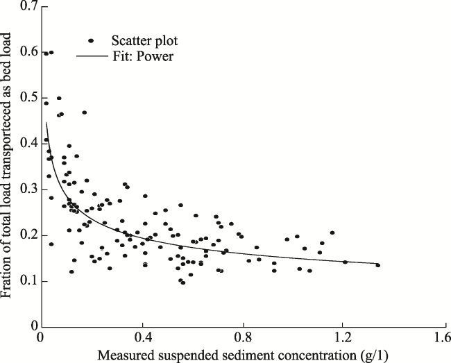
Figure 3 A typical covariation of the proportion of total load conveyed as bed load with observed suspended sediment concentration at Kantamal |
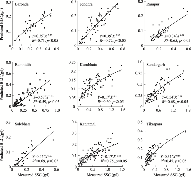
Figure 4 Variation of the predicted ungauged bed load concentration (BLCu) and gauged suspended sediment concentration (SSCg) across stations (Solid black lines denote the fitted power regression, and p defines the probability of significance) |
Table 11 Error statistics of the proposed power regression model at various stations |
| Stations | NSE | RSR | PBIAS (%) | Stations | NSE | RSR | PBIAS (%) |
|---|---|---|---|---|---|---|---|
| Baronda | 0.63 | 0.60 | 2.28 | Sundargarh | 0.68 | 0.56 | 5.82 |
| Jondhra | 0.68 | 0.55 | 4.60 | Salebhata | 0.80 | 0.43 | 10.59 |
| Rampur | 0.69 | 0.55 | 4.65 | Kantamal | 0.69 | 0.54 | 7.48 |
| Bamnidih | 0.72 | 0.52 | 15.21 | Tikarpara | 0.57 | 0.64 | 8.82 |
| Kurubhata | 0.58 | 0.64 | 0.44 |
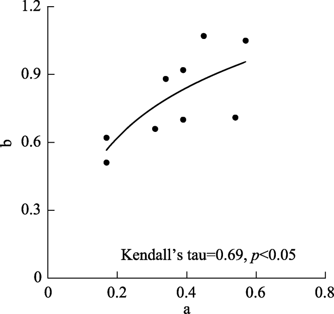
Figure 5 Association between the constants of the proposed relations between SSCg and BLCu (Solid black line indicates the nonlinear trend, and p defines the probability of significance) |
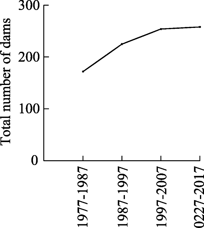
Figure 6 Variation of the construction of large dams in the river basin in the ten-year interval from 1977-2017 |
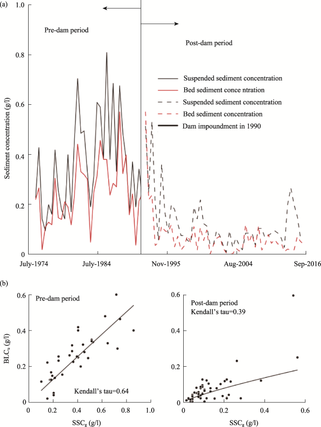
Figure 7 Impact of the Bango dam impoundment (1990) on the (a) variation of bed and suspended sediment concentration and (b) correlation between the bed (BLCu) and suspended sediment concentration (SSCg), as observed at Bamnidih |
Figure 8 Graphical summary of Discrepancy ratio (DRa) across all stations, where the observations between the solid black lines are considered within acceptable limits, and black dotted lines represent the line of perfect agreement |
Table 12 Statistical performance of different bed load functions (BLFs) across stations of the basin |
| Stations | BLFs | DRa | Score (%) | DI | IC |
|---|---|---|---|---|---|
| Baronda | Shields 1936 | 3984609 | 0 | 1.59×10¹³ | 0.99 |
| Schoklitsch 1962 | 4.88 | 12.50 | 18.94 | 0.52 | |
| Bagnold 1980 | 0.82 | 56.25 | 1.46 | 0.40 | |
| Roorkee | 1.89 | 62.50 | 3.57 | 0.36 | |
| Julien 2002 | 214.88 | 0 | 45960.89 | 0.98 | |
| Huang 2010 | 1.12 | 56.25 | 2.59 | 0.35 | |
| Recking 2013 | 564.30 | 0 | 317907.74 | 0.99 | |
| Jondhra | Shields 1936 | 2163377.34 | 0 | 4.68×10¹² | 0.99 |
| Schoklitsch 1962 | 1.73 | 77.94 | 2.13 | 0.22 | |
| Bagnold 1980 | 0.36 | 16.17 | 3.56 | 0.69 | |
| Roorkee | 6.31 | 45.58 | 34.27 | 0.58 | |
| Julien 2002 | 68.20 | 0 | 4583.21 | 0.95 | |
| Huang 2010 | 4.01 | 64.70 | 14.12 | 0.47 | |
| Recking 2013 | 2.47 | 23.52 | 14.15 | 0.74 | |
| Rampur | Shields, 1936 | 1.38×10⁸ | 0 | 1.91×10¹⁶ | 1 |
| Schoklitsch 1962 | 51.06 | 0 | 2556.37 | 0.984 | |
| Bagnold 1980 | 8.84 | 0 | 69.45 | 0.74 | |
| Roorkee | 2.48 | 42.50 | 4.23 | 0.41 | |
| Julien 2002 | 6383.28 | 0 | 40739959.30 | 0.99 | |
| Huang 2010 | 1.34 | 65 | 1.32 | 0.32 | |
| Recking 2013 | 9285.78 | 0 | 86216436.35 | 0.99 | |
| Bamnidih | Shields 1936 | 2287781.84 | 0 | 5.23×10¹² | 0.99 |
| Schoklitsch 1962 | 1.88 | 63.49 | 2.36 | 0.28 | |
| Bagnold 1980 | 0.28 | 19.04 | 3.98 | 0.76 | |
| Roorkee | 1.61 | 57.14 | 2.57 | 0.28 | |
| Julien 2002 | 198.10 | 0 | 39047.07 | 0.97 | |
| Huang 2010 | 0.85 | 41.26 | 1.99 | 0.40 | |
| Recking 2013 | 152.44 | 1.58 | 23087.79 | 0.98 | |
| Kurubhata | Shields 1936 | 3511056.36 | 0 | 1.23×10¹³ | 0.99 |
| Schoklitsch 1962 | 2.42 | 50.63 | 3.45 | 0.33 | |
| Bagnold 1980 | 0.55 | 37.97 | 1.34 | 0.45 | |
| Roorkee | 0.82 | 72.15 | 1.05 | 0.29 | |
| Julien 2002 | 109.90 | 0 | 11968.71 | 0.97 | |
| Huang 2010 | 0.47 | 32.91 | 2.24 | 0.47 | |
| Recking 2013 | 156.60 | 0 | 24367.13 | 0.99 | |
| Sundargarh | Shields 1936 | 24937514.25 | 0 | 6.22×10¹⁴ | 1 |
| Schoklitsch 1962 | 7.66 | 2.59 | 51.04 | 0.64 | |
| Bagnold 1980 | 0.79 | 64.93 | 0.86 | 0.39 | |
| Roorkee | 0.86 | 48.05 | 1.63 | 0.43 | |
| Julien 2002 | 2451.75 | 0 | 6008655.03 | 0.99 | |
| Huang 2010 | 0.46 | 35.06 | 2.84 | 0.59 | |
| Recking 2013 | 2199.84 | 0 | 4837097.88 | 0.99 | |
| Salebhata | Shields 1936 | 7741251.25 | 0 | 7.34×10¹³ | 1 |
| Schoklitsch 1962 | 8.57 | 6.25 | 80.12 | 0.63 | |
| Bagnold 1980 | 1.76 | 53.12 | 3.24 | 0.36 | |
| Roorkee | 3.44 | 46.87 | 27 | 0.55 | |
| Julien 2002 | 331.08 | 0 | 124870.37 | 0.98 | |
| Huang 2010 | 1.81 | 50 | 10.42 | 0.49 | |
| Recking 2013 | 464.49 | 0 | 214443.40 | 0.99 | |
| Kantamal | Shields 1936 | 28790604.46 | 0 | 5.98×10¹⁴ | 1 |
| Schoklitsch 1962 | 10.6 | 0 | 72.84 | 0.72 | |
| Bagnold 1980 | 1.94 | 70.54 | 1.32 | 0.25 | |
| Roorkee | 1.66 | 59.60 | 2.39 | 0.36 | |
| Julien 2002 | 885.01 | 0 | 807412.07 | 0.99 | |
| Huang 2010 | 1.01 | 60.46 | 1.67 | 0.40 | |
| Recking 2013 | 374 | 8.52 | 754199.84 | 0.99 | |
| Tikarpara | Shields 1936 | 14290344.01 | 0 | 2.04×10¹⁴ | 1 |
| Schoklitsch 1962 | 3.72 | 22.64 | 10.20 | 0.44 | |
| Bagnold 1980 | 0.59 | 42.45 | 1.41 | 0.50 | |
| Roorkee | 0.73 | 37.73 | 4.22 | 0.49 | |
| Julien 2002 | 513.68 | 0 | 263359.66 | 0.99 | |
| Huang 2010 | 0.43 | 22.64 | 16.27 | 0.60 | |
| Recking 2013 | 2.61 | 32.07 | 20.88 | 0.62 |
| [1] |
|
| [2] |
|
| [3] |
|
| [4] |
|
| [5] |
|
| [6] |
|
| [7] |
|
| [8] |
|
| [9] |
|
| [10] |
|
| [11] |
|
| [12] |
|
| [13] |
|
| [14] |
|
| [15] |
|
| [16] |
|
| [17] |
|
| [18] |
|
| [19] |
|
| [20] |
|
| [21] |
|
| [22] |
|
| [23] |
|
| [24] |
|
| [25] |
CWC, 2014. Mahanadi Basin. Ministry of Water Resources: Govt. of India.
|
| [26] |
|
| [27] |
|
| [28] |
|
| [29] |
|
| [30] |
|
| [31] |
|
| [32] |
|
| [33] |
|
| [34] |
|
| [35] |
|
| [36] |
|
| [37] |
|
| [38] |
|
| [39] |
|
| [40] |
|
| [41] |
|
| [42] |
|
| [43] |
|
| [44] |
|
| [45] |
|
| [46] |
|
| [47] |
|
| [48] |
|
| [49] |
|
| [50] |
|
| [51] |
|
| [52] |
|
| [53] |
|
| [54] |
|
| [55] |
|
| [56] |
Kazemi, 2011. Estimating the bed load to suspended load ratio in Central Alborz Rivers, Iran (Case Study: Taleghan and Jajroud rivers). International Journal of Agriculture: Research and Review, 1(1): 44-47.
|
| [57] |
|
| [58] |
|
| [59] |
|
| [60] |
|
| [61] |
|
| [62] |
|
| [63] |
|
| [64] |
|
| [65] |
|
| [66] |
|
| [67] |
|
| [68] |
|
| [69] |
|
| [70] |
|
| [71] |
|
| [72] |
|
| [73] |
|
| [74] |
|
| [75] |
|
| [76] |
NRLD, 2018. National register of large dams. New Delhi: Government of India.
|
| [77] |
|
| [78] |
|
| [79] |
|
| [80] |
|
| [81] |
|
| [82] |
|
| [83] |
|
| [84] |
|
| [85] |
|
| [86] |
|
| [87] |
|
| [88] |
|
| [89] |
|
| [90] |
|
| [91] |
|
| [92] |
|
| [93] |
|
| [94] |
|
| [95] |
|
| [96] |
|
| [97] |
|
| [98] |
|
| [99] |
|
| [100] |
|
| [101] |
|
| [102] |
|
| [103] |
|
| [104] |
|
| [105] |
|
| [106] |
|
| [107] |
|
| [108] |
|
| [109] |
|
| [110] |
|
| [111] |
|
/
| 〈 |
|
〉 |
