
Journal of Geographical Sciences >
Spatiotemporal variations in remote sensing phenology of vegetation and its responses to temperature change of boreal forest in tundra- taiga transitional zone in the Eastern Siberia
|
Li Cheng (1991-), PhD, specialized in applications of remote sensing of resources and environment and geographic information system. E-mail: licheng@lreis.ac.cn |
Received date: 2022-08-20
Accepted date: 2022-10-25
Online published: 2023-03-21
Supported by
Major Special Project-The China High-Resolution Earth Observation System(30-Y20A07-9003-17/18)
Phenology is an important indicator of climate change. Studying spatiotemporal variations in remote sensing phenology of vegetation can provide a basis for further analysis of global climate change. Based on time series data of MODIS-NDVI from 2000 to 2017, we extracted and analyzed four remote sensing phenological parameters of vegetation, including the Start of Season (SOS), the End of Season (EOS), the Middle of Season (MOS) and the Length of Season (LOS), in tundra-taiga transitional zone in the East Siberia, using asymmetric Gaussian function and dynamic threshold methods. Meanwhile, we analyzed the responses of the four phenological parameters to the temperature change based on the temperature change data from Climate Research Unit (CRU). The results show that: in regions south of 64°N, with the rise of temperature in April and May, the SOS in the corresponding area was 5-15 days ahead of schedule; in the area between 64°N and 72°N, with the rise of temperature in May and June, the SOS in the corresponding area was 10-25 days ahead of schedule; in the northernmost of the study area on the coast of the Arctic Ocean, with the drop of temperature in May and June, the SOS in the corresponding area was 15-25 days behind schedule; in the northwest of the study area in August and the southwest in September, with the drop of temperature, the EOS in the corresponding areas was 15-30 days ahead of schedule; in regions south of 67°N, with the rise of temperature in September and October, the EOS in the corresponding area was 5-30 days behind schedule; the change of the EOS in autumn was more sensitive to the change of the SOS in spring, because the smaller temperature fluctuation can cause the larger change of the EOS; the growth season of vegetation in the study area was generally moving forward, and the LOS in the northwest was shortened, while the LOS in the middle and south of the study area was prolonged.
Key words: phenology; climate change; Siberia; asymmetric Gaussian function; GeoDetector
LI Cheng , ZHUANG Dafang , HE Jianfeng , WEN Kege . Spatiotemporal variations in remote sensing phenology of vegetation and its responses to temperature change of boreal forest in tundra- taiga transitional zone in the Eastern Siberia[J]. Journal of Geographical Sciences, 2023 , 33(3) : 464 -482 . DOI: 10.1007/s11442-023-2092-z
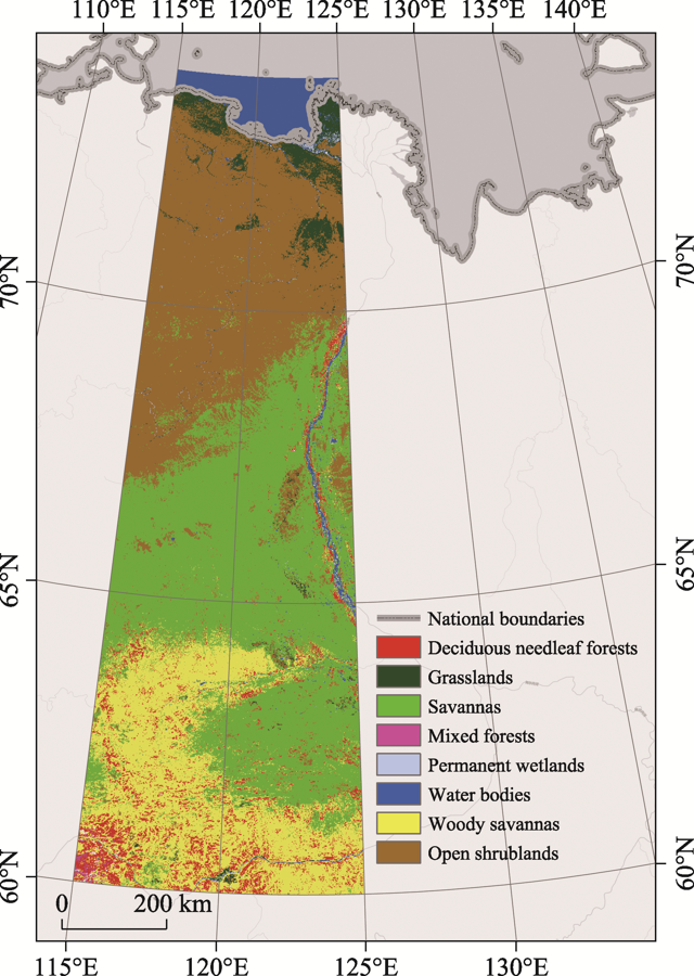
Figure 1 Scope and land cover types of the study area in the Eastern Siberia |
Table 1 Definition of Vegetation growth season parameters extracting from NDVI data |
| Vegetation growth season parameter | Definition |
|---|---|
| The start of the season (SOS) | Time for which the left edge has increased to 10% measured from the left minimum level. |
| The end of the season (EOS) | Time for which the right edge has decreased to 10% measured from the right minimum level. |
| The mid of the season (MOS) | Computed as the mean value of the times for which, respectively, the left edge has increased to the 80 % level and the right edge has decreased to the 80 % level. |
| Length of the season (LOS) | Time from the start to the end of the season. |
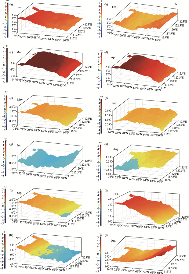
Figure 2 Spatial distribution of monthly average temperature in the study area between 2000 and 2017 |
Figure 3 Linear trend of monthly average temperature in the study area between 2000 and 2017 |
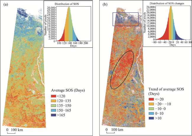
Figure 4 Spatial distribution (a) and the linear trend (b) of average SOS in the study area from 2000 to 2017 |
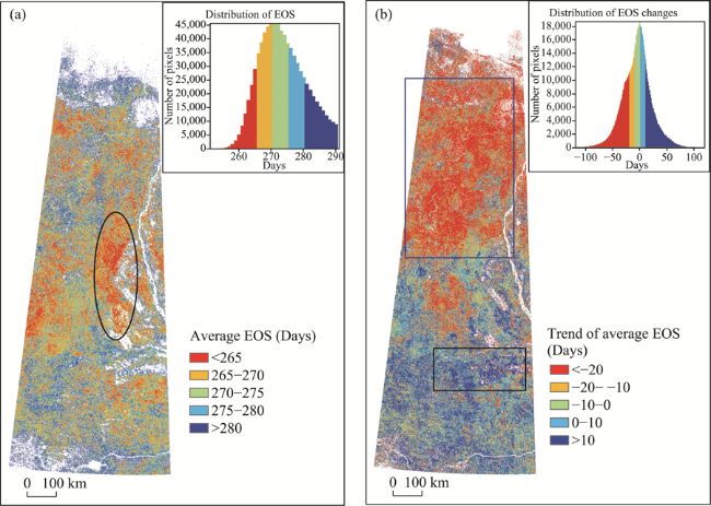
Figure 5 Spatial distribution of average EOS (a) and the linear trend of EOS (b) in the study area from 2000 to 2017 |
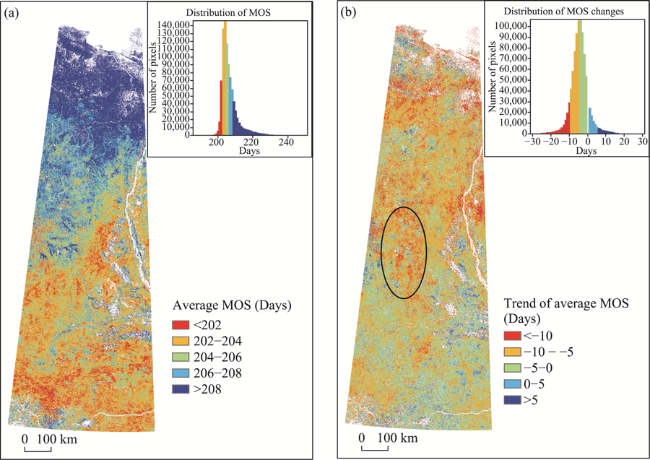
Figure 6 Spatial distribution of average MOS (a) and the linear trend of MOS (b) in the study area from 2000 to 2017 |
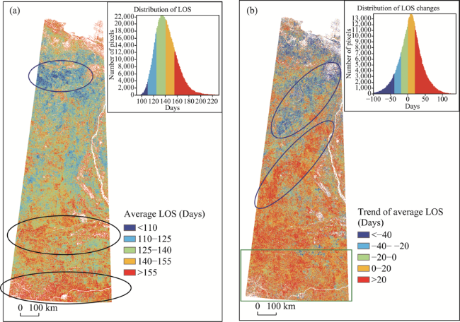
Figure 7 Spatial distribution of average LOS (a) and the linear trend of LOS in the study area from 2000 to 2017 |
| [1] |
|
| [2] |
|
| [3] |
|
| [4] |
|
| [5] |
|
| [6] |
|
| [7] |
|
| [8] |
|
| [9] |
|
| [10] |
|
| [11] |
|
| [12] |
|
| [13] |
|
| [14] |
|
| [15] |
|
| [16] |
|
| [17] |
|
| [18] |
|
| [19] |
|
| [20] |
|
| [21] |
|
| [22] |
|
| [23] |
|
| [24] |
|
| [25] |
|
| [26] |
|
| [27] |
|
| [28] |
|
| [29] |
|
| [30] |
|
| [31] |
|
| [32] |
|
| [33] |
|
| [34] |
|
| [35] |
|
| [36] |
|
| [37] |
|
| [38] |
|
/
| 〈 |
|
〉 |
