Special Issue: Land for High-quality Development

Exploring detailed urban-rural development under intersecting population growth and food production scenarios: Trajectories for China’s most populous agricultural province to 2030

  • GAO Peichao , 1, 2 ,
  • XIE Yiru 3 ,
  • SONG Changqing , 2, * ,
  • CHENG Changxiu 2, 4 ,
  • YE Sijing 2
Expand
  • 1. State Key Laboratory of Earth Surface Processes and Resource Ecology, Beijing Normal University, Beijing 100875, China
  • 2. Faculty of Geographical Science, Beijing Normal University, Beijing 100875, China
  • 3. Key Laboratory of Environmental Change and Natural Disaster, Beijing Normal University, Beijing 100875, China
  • 4. National Tibetan Plateau Data Center, Beijing 100101, China
*Song Changqing (1961−), Professor, specialized in geographical paradigms and regional integration. E-mail:

Gao Peichao (1991−), Assistant Professor, specialized in information geography. E-mail:

Received date: 2021-06-01

  Accepted date: 2021-11-29

  Online published: 2023-02-21

Supported by

Strategic Priority Research Program of the Chinese Academy of Sciences(XDA23100303)

National Natural Science Foundation of China(42271418)

National Natural Science Foundation of China(42171250)

National Natural Science Foundation of China(42230106)

State Key Laboratory of Earth Surface Processes and Resource Ecology(2022-ZD-04)

Copyright

© 2023

Abstract

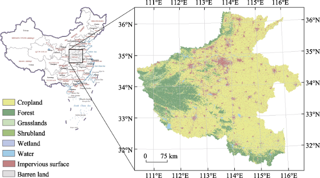
Henan, China, is likely the most populous agricultural province worldwide. It is China’s major grain-producing area, with a continuously increasing population (96 million), which is greater than 93% of countries worldwide. However, this province has been experiencing unprecedented urbanization recently due to national policies and measures, such as a plan to build the capital city of Henan into a national center, resulting in severe conflicts in land use that endanger food security regionally and globally. To facilitate decision-making on this problem, we explored the detailed urban-rural development of Henan by modeling these land-use conflicts. Conventional modeling of a region’s urban-rural development is to navigate trade-offs (a) solely between different land-use types (b) by assuming that each type provides a single service (e.g., croplands produce all the food), and (c) under a polynomial regression-based projection of population. In contrast, we considered both land-use type and intensity, resulting in a detailed land system for Henan. By introducing the concept of land system services (e.g., food production), we established a many-to-many relationship between land system classes and services. These allowed us to carry out the most comprehensive modeling of Henan’s urban-rural development under eighteen combined scenarios of population growth and land-use policies on food production. The modeling results of these scenarios provide a solid basis for making decisions regarding Henan’s urban-rural development. We also revealed the influence mechanism of population growth, land-use policies, and their combinations, highlighting the benefits of securing food production by agricultural intensification rather than merely expanding the area of cropland.

Cite this article

GAO Peichao , XIE Yiru , SONG Changqing , CHENG Changxiu , YE Sijing . Exploring detailed urban-rural development under intersecting population growth and food production scenarios: Trajectories for China’s most populous agricultural province to 2030[J]. Journal of Geographical Sciences, 2023 , 33(2) : 222 -244 . DOI: 10.1007/s11442-023-2080-3

1 Introduction

Located in the Yellow River Valley and with over 5000 years of recorded history, Henan Province is widely considered the cradle of Chinese civilization. Among the most agriculturally productive areas of China, it feeds a large population. According to the National Bureau of Statistics of China (NBSC, 2019a), its food production in 2019 was 67 million tons, ranking second out of all 31 statistical units, following the most agriculturally productive province, Heilongjiang, which has a food production of 75 million tons. In contrast, the populations of Henan and Heilongjiang are 96 and 38 million, respectively, according to the latest published statistics (NBSC, 2019b). Therefore, Henan is China’s most populous agricultural province, and given its large population, it is likely the most populous agricultural province worldwide.
Since the population of both Henan and all of China is expected to continue increasing (Deng et al., 2015), many efforts are required to ensure food security by narrowing the gap between a growing population and rising food demand (e.g., Jin et al., 2020; Tang et al., 2021). Usually, food production can be increased by converting diverse land-use types to cropland (Kuang, 2019; Peng et al., 2020), which offers a solution for Henan. However, Henan faces a surge in demand for construction land because promoting central China’s (including Henan) urban and rural development has recently become a focus for the whole country. A series of policies and measures have been launched by the central government, such as the strategy for the rise of central China, which is a plan to build the capital city of Henan into a national central city (similar to Beijing and Shanghai), and the high-quality economic development of the Yellow River Basin. As a result, land-use conflicts have become increasingly prevalent in Henan, so trade-offs should be considered (e.g., Jin et al., 2018; Sun et al., 2018; Peng et al., 2019a; 2019b; Wang et al., 2019b; Dai et al., 2020).
The current study aimed to progress the consideration of such trade-offs by exploring Henan’s urban-rural development trajectories under intersecting population growth and food production scenarios. This exploration is, however, challenging for three reasons. First, population growth in Henan increases the demand for both food and accommodation. Efforts to meet the former demand result in more cropland and/or agricultural intensification, whereas efforts to meet the latter lead to urbanization and/or the development of rural settlements. It can be seen the results of these efforts are generally conflicting. According to Liu et al. (2010), most croplands in China have been lost due to urbanization and the development of rural settlements. Second, we needed to consider both the type and intensity of land use/cover. Third, the conversion of land use/cover may be subject to constraints, such as land-use policies on food production (Gao et al., 2021a). To the best of our knowledge, no previous attempts have been made toward this specific aim or to model Henan’s urban and/or rural change trajectories.
In this study, we have three specific research questions. First, how can the land changes in Henan be projected by considering both the types and intensity of land use/cover? Second, what are the future trajectories of Henan’s urban-rural development as a trade-off of population growth and food security? Third, how can land-use conflicts regarding land-use policy on food production be address in the projection?

2 Study area and related works

2.1 Study area: Henan, China

Henan, a landlocked Chinese province, is located between 31°-36°N and 110°-116°E (Ma et al., 2008). Its neighboring provinces are Shaanxi (west), Shanxi (northwest), Hebei (north), Shandong (northeast), Anhui (southeast), and Hubei (south). Henan has a relatively small geographical area but a large population. Its total area is approximately 167,000 km2, constituting only 1.7% of the total land area of China and ranking 17th out of all 34 Chinese provincial-level regions. In contrast, Henan is among the most populous provinces in China, ranking second or third over the last decade. Its population is nearly 100 million, which is greater than that of most countries worldwide. Its population constitutes more than 7% of China’s total population.
The climate in Henan is suitable for crop growth, with an average annual temperature range of 12.7-16.2℃, an average annual precipitation range of 478-1167 mm, an average annual sunshine hour range of 1468-2247, and an average annual frost-free period (i.e., growing period) range of 208-272 days. As a result, Henan’s lands are dominantly used as cropland (Figure 1). The province is one of the major grain-producing areas of China, ranking first in food production among all provinces before 2009 and second since 2010.
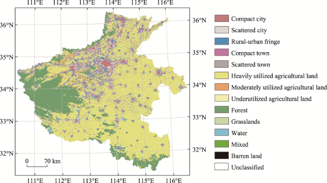
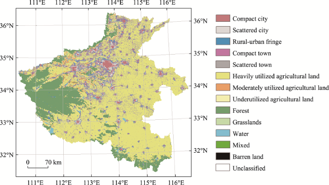
Figure 1 Land use in Henan province in 2017 (spatial resolution: 10 m; derived from Gong et al., 2019)

2.2 Related works

To the best of our knowledge, no previous attempts have been made toward this specific aim or to model Henan’s urban and/or rural change trajectories. However, considerable research has been focused on other areas worldwide. Examples of such research are the estimation of land-use/cover changes in the Dwarakeswar-Gandheswari river basin, India (Sahoo et al., 2018), the prediction of urban expansion in the Moscow region, Russia (Vasenev et al., 2018), and the simulation of land-use change in the southeast coastal region of China to identify future land-use conflicts (Zou et al., 2019). More recent examples include a prediction of future wetland areas in an India-Bangladesh river basin (Talukdar and Pal, 2020) and simulations of China’s land-use changes under policy constraints (Li and Chen, 2020) or different management scenarios (Zhu et al., 2020).
The current study differs from previous research efforts in three ways. First, future trajectories of urban-rural development were explored in terms of not only land-use type but also land-use intensity; for example, croplands were divided into high, medium, and low levels of productivity. This land-use classification, referred to as a detailed land system in the current study, allows for a more explicit description of urban-rural development. Second, a new concept was introduced, land system services, whereby a land system class can be defined as providing multiple land system services. This allowed for the establishment of many-to-many relationships between land system classes and services. For example, food production comes from not only cropland—which is the case in most previous studies—but also from urban areas. Third, population growth was considered more scientifically than in previous studies, using the five shared socioeconomic pathways (SSPs) developed by the Intergovernmental Panel on Climate Change (Riahi et al., 2017).

3 Methodology

3.1 A detailed land system: Raw data and system establishment

To consider both the type and intensity of land use/cover, we established a detailed land system, a highlight of this paper. In landscape ecology, such a detailed land system can be understood as a combination of landscape mosaics (Shaker et al., 2019; Zhang et al., 2020; Gao et al., 2021b) and gradients (McGarigal and Cushman, 2005; Gao et al., 2017; 2019). Intensity is quantified using either the property of a land-use/cover type, such as the food production of cropland, or the proportion of a specific land-use/cover type in a landscape mosaic cell.
To establish a detailed land system, we first prepared high-resolution land-cover data for Henan from the latest 10-m resolution global land-cover dataset, FROM-GLC10 (Finer Resolution Observation and Monitoring of Global Land Cover 10 m), Version 0.1.3 (Gong et al., 2019), as shown in Figure 1. Note that FROM-GLC10 has the highest spatial resolution among various useful land-use/cover data products (e.g., Kuang and Dou, 2020). The FROM-GLC10 dataset includes ten types of land cover, namely, cropland, forest, grasslands, shrubland, wetland, water, tundra, impervious surface, barren land, and snow/ice, as described in detail by Gong et al. (2013). Henan contains eight of these ten land cover types; it contains no tundra or snow/ice.
Then, we designed the framework of the detailed land system according to the research questions (Section 1) and original types of the high-resolution land-cover data. It consists of four primary categories and a total of 16 land classes. The first category, human settlement, consists of compact city, scattered city, urban-rural fringe, compact town, and scattered town. The second category is agriculture, comprising heavily utilized, moderately utilized, and underutilized agricultural land. The third category is environment, comprising forest, grasslands, shrubland, wetland, water, and mixed. These three categories have also been employed in other studies of land-use dynamics (e.g., Kirch et al., 2004). The fourth category consists of barren land and others (i.e., unclassified).
With this designed framework, a detailed land system was established by upscaling the high-resolution land-cover data from a spatial resolution of 10 m to 1 km. To perform upscaling, a set of classification rules (Figure 2) iteratively developed according to expert experiences. Specifically, we first performed upscaling using a set of subjective rules. Then, the result of the upscaling was investigated at the 1-km pixel level (formal results will be shown later in Figure 5). The investigation was made to see the components, which were a great number of 10-m pixels, and their proportions. If the composition of a 1-km pixel did not match the name of its corresponding land class, then the rules were refined, and upscaling was reperformed. An example of mismatch can be as follows: A 1-km pixel of the land class “underutilized agricultural land” consisted of all 10-m pixels of cropland.
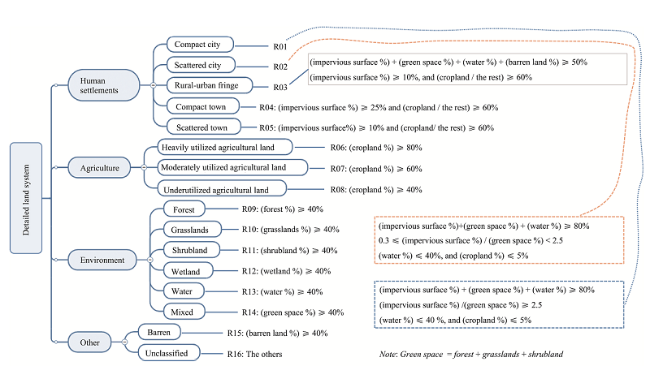
Figure 2 Classification scheme for the detailed land system

3.2 Many-to-many relationships between land classes and services

We first defined land system services and then established a many-to-many relationship between land system services and classes by identifying and quantifying the multiple services of different land system classes.
Readers may be familiar with the concept of ecosystem services, which refer to the goods (e.g., air, water, and food) and services (e.g., tourism, spiritual experience, and aesthetic provision) that ecosystems provide for humans (Wallace 2007). In the paradigm of ecosystem services research, an ecosystem is usually specified in terms of type (e.g., aquatic or terrestrial) or scale (e.g., regional or national). In the current study, we proposed a similar but distinctly different concept and paradigm: land system services. We defined this concept as the goods and services that a land system provides for humans, whereby a land system is specified in terms of land-use/cover type and intensity. Note that the term “land system services” has been occasionally used in the literature without formal definition (Eitelberg et al., 2016; Debonne et al., 2018; Ellis et al., 2019). This study presents the first formal definition.
Before quantifying land system services (i.e., quantifying the capability of each land class to provide every service), we need to identify key demands as the driving factors of land system change. As shown in Figure 3, the expected growth of Henan’s population will increase two conflicting human demands: accommodation and food. Human demand for accommodation is a major driving force of the conversion of agricultural to urban-rural land systems (Long et al., 2009; Ahmed et al., 2014; Lan et al., 2019), whereas the human demand for food can drive the expansion or intensification of agricultural land systems (Grundy et al., 2016; Delzeit et al., 2017). In this study, both accommodation and food were identified as the key demands, as well as cropland. Cropland is also of interest because it is a good proxy for the demand for food and can be used to analyze land-use policies in this study (will be shown in sections 5-6; either to expand the area of agricultural land systems, i.e., heavily/moderately/underutilized agricultural land, or to intensify the use of agricultural land systems, e.g., convert underutilized agricultural land to moderately or heavily utilized).
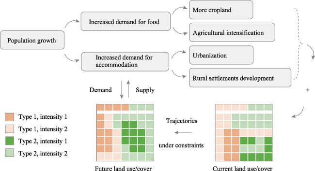
Figure 3 Population-driven changes in land use as the exploration framework
Then, we quantified the capability of every land class to provide each of these three land system services. In other words, each of the 16 land classes modeled in this study (Figure 2) was assumed to have the capability of providing accommodation, food, and cropland services to some extent, to meet the three key demands. The quantification was performed as follows:
·Land system services for accommodation (ai) were quantified using the population of each land system class, which was estimated using the highest-resolution dataset available for the spatial distribution of the population and then corrected using official statistics. This quantification process involved five steps. First, we obtained the Global Human Settlement Layer (GHSL) for the latest available year with the finest resolution (Pesaresi et al., 2013; Freire et al., 2016), that is, GHSL 2015 (250 m). Second, the GHSL dataset was overlaid with the detailed land system to derive the total population of Henan (P) and the population of each Henan land system class (Pi). Third, the data for Henan’s population (P°) in 2017 were obtained from the statistical yearbook released by the Henan Bureau of Statistics (2018). Fourth, every Pi was corrected as \[{{{P}'}_{i}}={{P}_{i}}\div P\times {P}'\]. Fifth, ai was determined using the following equation:
${{a}_{i}}=\frac{{{{{P}'}}_{i}}}{{{S}_{i}}}=\frac{{{P}_{i}}\cdot {P}'}{P\cdot {{N}_{i}}\cdot {{R}^{2}}}$
where Si and Ni are the total area (km2) and the total number of cells of the ith land system class in Henan, respectively, and 1:R(km) denotes the spatial resolution of the detailed land system. The ai units are persons per square kilometer (km2).
·Land system services for cropland (ci) were quantified as the total area of cropland included in a single cell of each land system class. This quantification was achieved by overlaying the detailed land system and the high-resolution land-cover data for Henan and then employing the following equation:
${{c}_{i}}=\frac{{{r}^{2}}}{{{N}_{i}}\cdot {{R}^{2}}}\underset{j=1}{\overset{{{N}_{i}}}{\mathop \sum }}\,{{c}_{ij}}$
To facilitate the explanation of cij, let us refer to the cropland cells of the high-resolution land-cover data for Henan as small cropland cells. Accordingly, cij is the total number of small cropland cells that are overlaid with the jth cell of the ith class of the detailed land system. 1:r(km) denotes the spatial resolution of the high-resolution land-cover data for Henan. The units of ci are km2/km2
·Land system services for food (${{f}_{i}}$) were quantified as the grain production (t) per square kilometer of the $i$th land system class using the following equation:
${{f}_{i}}=\frac{{{r}^{2}}}{{{N}_{i}}\cdot {{R}^{2}}}\underset{j=1}{\overset{{{N}_{i}}}{\mathop \sum }}\,\underset{k=1}{\overset{{{c}_{ij}}}{\mathop \sum }}\,{{f}_{ijk}}$
where fijk is the grain production (t) of the kth (1≤kcij) small cropland cell that is overlaid with the jth cell of the ith class of the detailed land system. The value of fijk depends on the spatial resolution of the data on grain production. To the best of our knowledge, the highest-resolution data available are the county-level (158 counties in total) grain production data of Henan in 2017 (HBS, 2018). Therefore, the determination of fijk was performed as follows. First, we divided the grain production of each county by its total area of cropland to derive the average grain production of the cropland of each county. Second, the value of fijk equals the average grain production of the cropland of a county if the small cropland area belongs to that county.

3.3 Scenario design based on population growth and land-use policy

We developed a total of eighteen scenarios by combining six population projections and three land-use policies. Six population projections were adopted for two reasons. First, population growth was regarded as the initial driving force of land system changes, as previously shown in Figure 3. Second, these six projections serve as the most comprehensive prediction of population changes under different representative assumptions, as will be explained in this section. Of these population projections, five were estimated by Chen et al. (2020) under the SSPs (shared socioeconomic pathways) or, more specifically, five SSP-based demographic assumptions specific to Chinese provinces. The five SSPs were developed by the Intergovernmental Panel on Climate Change (O’Neill et al., 2014; Liao et al., 2020) as descriptions of the world’s future in five assumptions, namely, sustainable development, business-as-usual, global/regional rivalry, inequality, and fossil-fueled development. The corresponding five SSP-based demographic assumptions by Chen et al. (2020) differed in fertility rate, mortality rate, interprovincial migration, educational attainment, and China’s fertility policy (i.e., two-child policy, fully open policy, or none), as summarized in Table 1. However, these SSP-based population projections were initially based on 2010 population data, which is a different reference year from that of the current study, namely, 2017. Therefore, we calibrated these projections for our research period, 2017-2030, using the actual population of Henan in 2017, as shown in Table 2. To the best of our knowledge, this study is the first of its kind to employ SSP-based population projections at China’s provincial level and consider China’s latest fertility policy, namely, the two-child policy launched in 2016 that allows all families to have two children (rather than only one, as before).
Table 1 Comparison of the five SSP-based demographic assumptions (Chen et al., 2020)
No. Framework Fertility rate Mortality Migration Education Fertility policy
1 SSP1 Low Low Medium High None
2 SSP2 Medium Medium Medium Medium Two-child
3 SSP3 High High Low Low Fully open
4 SSP4 Low Medium Medium Medium None
5 SSP5 Low Low High High None
In addition to these five SSP-based population projections, we made another projection according to Henan’s latest population control plan (Government of Henan, 2017). This plan outlines controlled population growth from 2015 to 2030 as follows:
·The population was 107.22 million in 2015.
·The average annual rate of population growth should be limited to approximately 0.78% from 2016 to 2020, leading to a population of approximately 111.50 million in 2020.
·The average annual rate of population growth should be limited to approximately 0.03% from 2021 to 2030, leading to a population of approximately 115.00 million in 2030.
Using these specifications, we calculated the planned population of Henan from 2018 to 2030 using 2017 as the reference year, as shown in Table 2.
Table 2 Six projections for Henan’s population (in millions) from 2018 to 2030, with 2017 as the reference year
SSP1 SSP2 SSP3 SSP4 SSP5 Planned
2017 108.530 108.530 108.530 108.530 108.530 108.530
2018 109.221 109.325 109.440 109.199 109.187 109.377
2019 109.896 110.125 110.369 109.847 109.827 110.230
2020 110.555 110.930 111.315 110.475 110.448 111.089
2021 111.181 111.692 112.226 111.064 111.039 111.423
2022 111.775 112.412 113.103 111.615 111.603 111.757
2023 112.331 113.084 113.936 112.121 112.133 112.092
2024 112.851 113.707 114.724 112.582 112.631 112.429
2025 113.330 114.278 115.463 112.995 113.092 112.766
2026 113.768 114.796 116.154 113.360 113.516 113.104
2027 114.165 115.264 116.799 113.679 113.904 113.443
2028 114.517 115.677 117.394 113.947 114.249 113.784
2029 114.823 116.037 117.944 114.166 114.553 114.125
2030 115.085 116.345 118.449 114.337 114.815 114.467
For land-use policies, we considered three strategies concerning cropland: the total area of cropland remains stable, the food production of cropland remains stable, and no policies for cropland or its food production. It is important to note that in our study, both cropland and food can come from any land system class, including cities.
By combining different population projections and land-use policies, we obtained a total of eighteen scenarios, as shown in Table 3.
Table 3 Scenarios (S01-S18) designed by combining population projections and land-use policies
Land-use policies SSP1 SSP2 SSP3 SSP4 SSP5 Planned
P1: Area of cropland remains stable S01 S02 S03 S04 S05 S06
P2: Food production remains stable S07 S08 S09 S10 S11 S12
P3: No policies for cropland or food S13 S14 S15 S16 S17 S18

3.4 Explanatory factors for land dynamics: Selection through regression

To understand land dynamics, we first prepared a number of candidate factors and then tested their explanatory powers of historical land-use/cover change using regression analysis.
In preparing the candidate factors, we established three rules: the factor is or should be relevant to land dynamics, the factor data are easily accessible, and as many factors and categories as possible should be included. Using these three rules, we collected eight categories, a total of 27 candidate factors, summarized in Table 4.
Table 4 List of candidate factors
Category Factors Source
Socioeconomy 1 Gross domestic product DOI: 10.12078/2017121102
2 Nighttime lights Defense Meteorological Satellite Program
3 Population distribution Global Human Settlement
Accessibility 4 Accessibility to cities (Weiss et al., 2018)
5-8 Accessibility to rivers/lakes/ railways/roads Calculated from OpenStreetMap
Soil property 9 Bulk density 10 Clay content (Hengl et al., 2017)
11 Cation exchange capacity 12 pH in H2O
13 Organic carbon density 14 Sand content
15 Coarse fragments volumetric 16 Silt content
17 Water capacity 18 Texture class
Vegetation 19 NDVI DOI: 10.12078/2018060601
Agriculture 20 Potential crop yield DOI: 10.12078/2017122301
Temperature 21-22 Mean February/August temperature (Peng et al., 2019c)
Precipitation 23-24 Total May/September precipitation
Topography 25 Elevation Shuttle Radar Topography Mission
26-27 Slope/Aspect Calculated from elevation
We then performed a regression analysis between these candidate factors and the land system classes. To make the regression analysis more robust, we first removed highly correlated candidate factors. Specifically, we calculated the correlation coefficients between every pair of candidate factors. For any pair where the correlation coefficient was greater than 0.8, the member that was more correlated to all the other candidate factors was removed. By doing so, we removed the 23rd (total May precipitation) and 25th (elevation) candidate factors. The regression analysis was performed using a binomial logit model as follows:
$\log \left( \frac{{{P}_{i,j,k}}}{1-{{P}_{i,j,k}}} \right)={{\beta }_{0}}+{{\beta }_{1}}{{X}_{1,i,j}}+{{\beta }_{2}}{{X}_{2,i,j}}+\cdots +{{\beta }_{n}}{{X}_{n,i,j}}$
where Pi,j,k is the probability of the land unit (i,j) being the jth land system class; X1,i,j, X2,i,j, and Xn,i,j are the values of the first, second, and nth candidate factors for the land unit (i,j), respectively; and β0, β1, β2, and βn are the coefficients to be estimated.

3.5 Simulation model selection

Following the preceding design, we then needed a model to simulate changes to our detailed land system by considering the many-to-many relationship between supply (i.e., land classes) and demand (i.e., services). A number of available and frequently used models would have been suitable if the purpose was to only simulate changes in the detailed land system, for example, CLUE-S (Verburg et al., 2002; Bai et al., 2018), FLUS (Liu et al., 2017), LUSD-urban (He et al., 2017), LUTO (Gao and Bryan, 2017), SLEUTH (Chaudhuri and Clarke, 2019; Bajracharya et al., 2020), and Markov chain (Lu and Chen, 2017). However, to consider the many-to-many relationship between supply and demand, we chose the CLUMondo model. For readers interested in the principles and implementation of the CLUMondo model, please refer to publications by its developers (e.g., Pouzols et al., 2014; Eitelberg et al., 2016; van Vliet et al., 2017; Wolff et al., 2018; Debonne et al., 2019), especially their brief introduction to the beginners of the model (van Vliet and Verburg, 2018).

4 Results

4.1 Established detailed land system and quantified services

The detailed land system established for Henan is shown in Figure 4. It consists of 14 of the 16 initial land classes designed in the classification scheme (Figure 2). The proportion of each land class is shown in Table 5. The primary two categories of land class in Henan are agricultural land and urban-rural fringe. The spatial resolution of the established land system is 1 km, where every single pixel (Figure 5) was generated based on 100 pixels of the 10-m resolution Henan land-cover data (refer to Figure 1).
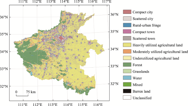
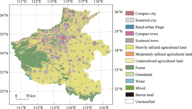
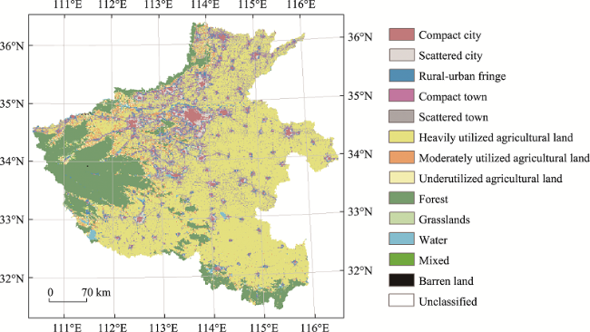
Figure 4 Detailed land system for Henan (spatial resolution: 1 km)
Table 5 Numbers and proportions of pixels for each class of detailed land system
Category No. Land class # of pixels Proportion (%) Sum (%)
Human settlements 1 Compact city 2742 1.65 21.65
2 Scattered city 2683 1.62
3 Urban-rural fringe 5067 3.05
4 Compact town 5235 3.16
5 Scattered town 20,203 12.17
Agriculture 6 Heavily utilized 82,117 49.48 58.56
7 Moderately utilized 8551 5.15
8 Underutilized 6527 3.93
Environment 9 Forest 30,288 18.25 19.69
10 Grasslands 752 0.45
11 Shrubland 0 0
12 Wetland 0 0
13 Water 1213 0.73
14 Mixed 437 0.26
Others 15 Barren land 23 0.02 0.10
16 Unclassified 137 0.08
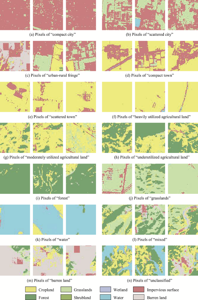
Figure 5 Detailed land system pixels (spatial resolution: 1 km; each subpicture is a single pixel in the system) and their components (spatial resolution: 10 m)
The quantified land system services are presented in Table 6. Each land class provides all three services. For example, the compact city class provides not only accommodation services but also food and cropland services, meaning that the expansion of a compact city can also lead to an increase in food and cropland. This type of many-to-many relationship between land classes and services is a highlight of this study.
Table 6 Services per square kilometer of each land system class
No. Land class Accommodation (persons) Food (tons) Cropland (km2)
a Compact city 6572.76 1.410 0.002349
b Scattered city 2139.43 1.682 0.002855
c Urban-rural fringe 2115.55 161.313 0.298364
d Compact town 1695.26 371.060 0.634181
e Scattered town 1114.86 490.878 0.809012
f Heavily utilized 450.65 578.799 0.944807
g Moderately utilized 286.74 285.485 0.706417
h Underutilized 170.87 191.109 0.498408
i Forest 45.50 34.881 0.095807
j Grasslands 456.12 34.245 0.111823
k Water 128.94 45.871 0.102480
l Mixed 344.39 100.857 0.319964
m Barren land 408.70 88.055 0.161213
n Unclassified 283.21 129.101 0.312731

4.2 Detailed land systems simulated for Henan in 2030

We simulated a detailed land system for Henan in 2030 under each of the 18 scenarios (Figure 6 and Appendix A). A quick comparison between the simulated detailed land systems (Figure 6) and the original (Figure 4) shows that they are similar from a macro perspective, demonstrating the inertia of land use (Wang et al., 2019a).
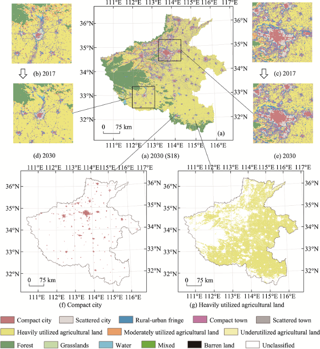
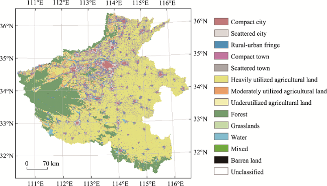
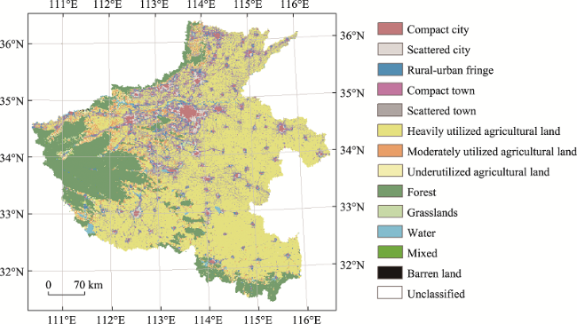
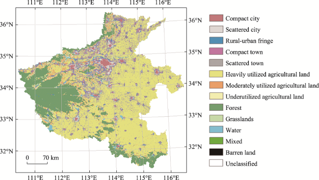
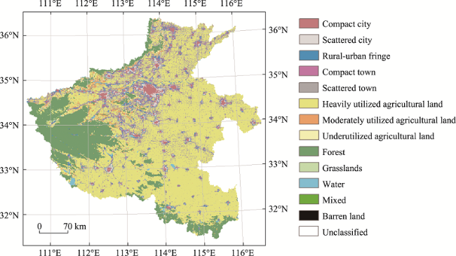
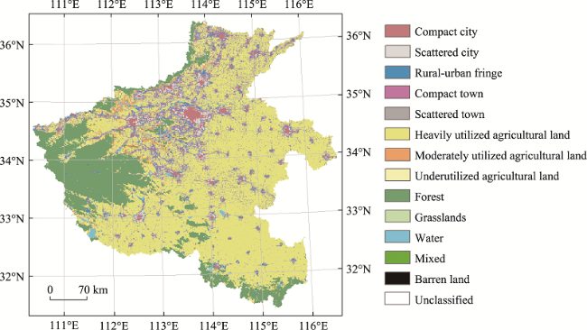
Figure 6 Detailed land system simulated for Henan in 2030 under S18 (a. The simulated system; b-e. Two comparisons between 2017 and 2030, and Distributions of (f) compact cities and (g) Heavily utilized agricultural land in the simulation system)
However, on closer inspection, we can observe changes in the land system between 2017 and 2030 in terms of not only the configuration (i.e., the spatial location of each class) but also the composition (i.e., the quantity of each class), as shown in the comparisons presented in Figures 6b-6e). To represent the configurational changes more accurately, we examined the proportions of cells where the land system class in 2030 differed from that in 2017, as shown in Figure 7. In addition, a more accurate comparison of the compositional changes is presented in Figure 8. Note that in making this figure, all land system classes from the categories of “environment” and “other” were combined and visualized as a single category, “natural,” because our focus was on the human settlement and agriculture categories.
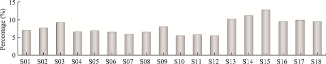
Figure 7 Proportions of cells where the land system class in 2030 differs from 2017 under all scenarios
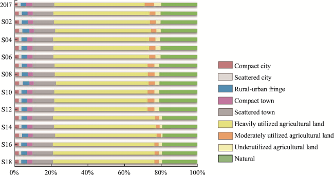
Figure 8 Comparison between the detailed land systems under 18 scenarios (S01-S18) and those of 2017 in terms of the composition of cells with different land system classes

4.3 Quantity and spatial distribution of land system services in 2030

The quantity of the three land system services in 2030 under each scenario is shown in Figure 9. Some general findings can be obtained. First, the amount of accommodation has improved in all scenarios to meet the needs of the growing population. Second, the quantity pattern shown by the cropland services of the 18 scenarios is similar to that of the food production services. This is understandable because food is produced from cropland. However, these two patterns are not identical, because croplands incorporated in different land system classes do not necessarily have the same production quantities. It is also important to note that two scenarios with the same (or similar) quantity of service do not necessarily correspond to the same (or similar) land system. For example, as shown in Figure 9(c), 2017 and S07 have similar food production quantities, but they have different compositions of land system classes, as previously shown in Figure 8, with different configurations (see Appendix A).
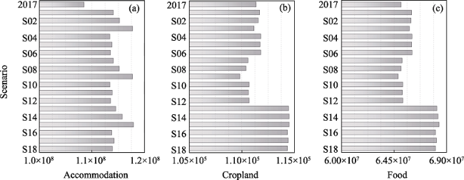
Figure 9 Quantity of services in 2030 (a. Accommodation; b. Cropland; c. Food)

5 Analysis and discussion

5.1 Response of land system classes to land-use policy and population

From the perspective of decision-makers, it is useful to understand the response of land system classes to different land-use policies and population projections. In this section, we first investigated the response to a combination of these two factors, namely, under each scenario. Then, we investigated the response to every single factor.
For the first investigation, we calculated the relative changes in the areas of each land system class from 2017 to 2030. Such calculations were performed for all 18 scenarios, as shown in Figure 10. The relative changes in these land system classes can be classified into three cases. The first case is “increase in all scenarios,” namely, compact city and heavily utilized (agricultural land). The second case is “decrease in all scenarios,” that is, compact town, moderately utilized, and underutilized (agricultural land). The third case is “increase/decrease in some scenarios,” which includes all the other land system classes. These three cases highlight the complexity of future land system changes.
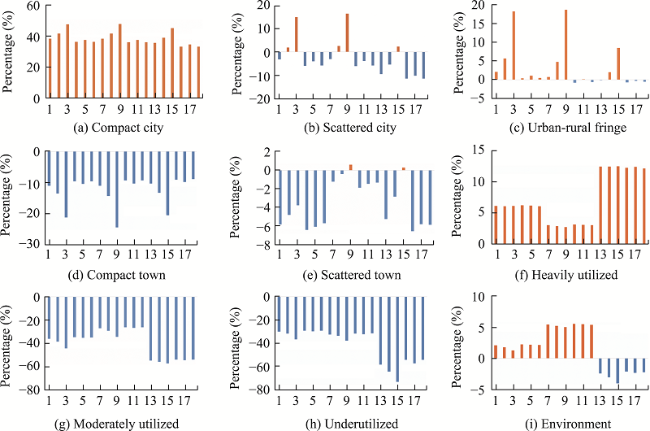
Figure 10 Relative changes in the areas of every land system class from 2017 to 2030 under each of the 18 scenarios
For the second investigation, we determined two sets of standard deviations for each land system class. One set was calculated by setting the land-use policy as the control variable and the population projection as the independent variable; the other set was calculated using the reverse setting: the population projection as the control variable and the land-use policy as the independent variable. For both sets, the standard deviation was treated as the dependent variable. All the results can be found in Appendix B, and Table 7 presents the results for the heavily utilized agricultural land. In Table 7, the data of the last column, “SD by row,” is the first set of standard deviations, and the data in the “SD by column” row is the second set. The land-use policy is the dominant factor driving the change in heavily utilized agricultural land because the second set of standard deviations is greater than the first set. A similar analysis was performed for all the other results to determine the dominant factor for each land system class, as shown in Table 8.
Table 7 Standard deviations (SDs) calculated using the land-use policy (P1-P3) as the control variable (SD by row) and using the population projection as the control variable (SD by column, %)
SSP1 SSP2 SSP3 SSP4 SSP5 Planned SD by row
P1 6.13 6.06 6.10 6.21 6.14 6.07 0.06
P2 3.00 2.87 2.69 3.14 3.06 3.03 0.16
P3 12.43 12.47 12.51 12.26 12.41 12.11 0.15
SD by column 4.80 4.89 4.99 4.64 4.77 4.62 -
Table 8 Dominant factor for each land system class
Dominant factor Land system class
Population growth (a) compact city, (b) scattered city
(c) urban-rural fringe, and (d) compact town
Land-use policy (e) scattered town, (f) heavily utilized, (g) moderately utilized,
(h) underutilized, and (i) environment

5.2 Effects of different land-use policies on the detailed land system

As already indicated by Figure 10, the three land-use policies have different effects on the urban-rural development of Henan. In this section, we discuss these effects in more detail.
Land-use policies had complex effects on the land system classes for the category of human settlement. As visualized in Figure 10 and shown in Appendix B, all three policies significantly increased (by at least one-third) the area of compact cities, although the amount of increase differed slightly. Given a population projection, the amount of increase was quite similar for land-use policies P1 and P2, both of which were slightly higher than that of P3 (e.g., 38.3%, 38.2%, and 35.5% for P1, P2, and P3, respectively, under SSP1). The three policies may either increase or decrease the area of the scattered city, but the following pattern can be obtained: The amount of change is similar for P1 and P2, both of which tend to increase more or decrease less than P3 (e.g., 14.9%, 16.4%, and 2.3% for P1, P2, and P3, respectively, under SSP3). For urban-rural fringes, P1 usually brings about a greater increase in the area than P2, and the same pattern was observed when P2 was compared with P3. In contrast, the different land-use policies had little effect on compact towns, although the amount of decrease for P3 was always the least. The area of scattered towns decreased in most of the scenarios (16 out of 18), except for two scenarios where the area increased slightly (less than 0.6%). Among all the scenarios, P1 usually resulted in the largest decrease, and P2 always produced the slightest decline.
The effects were more straightforward on the land system classes from the agricultural land category. All three land-use policies increased, decreased, and decreased the areas of heavily utilized, moderately utilized, and underutilized agricultural land, respectively. Specifically, for the land class “heavily utilized”, P3 brought about the largest increase in area, approximately 12% under any of the population projections. The increases brought about by P1 and P2 were stable for different population projections, being 6% and 3% on average, respectively. For the land class “moderately utilized”, P3 always resulted in the largest decrease, which was 1.5 times that of P1 and twice that with P2. For the land class “underutilized”, the effects of P1 and P2 made little difference; both brought about slighter decreases in area than P3.

5.3 Effects of differing population growth on the detailed land system

Different projections of population growth had differing effects on the land system classes from the category of human settlement. For the land classes “compact city”, “scattered city”, and “urban-rural fringe”, SSP3 brought about either the largest increase or the smallest decrease in area under any land-use policy, followed by SSP2, SSP1, SSP5, SSP6, and SSP4. In contrast, population growth had the opposite effect on the land class “compact town”; SSP6 resulted in the smallest decrease in area under any land-use policy, followed by SSP4, SSP5, SSP1, SSP2, and SSP3. For the land class “scattered town”, the effects of population growth varied with land-use policy but had the following common characteristics for any given policy: SSP3 and SSP2 brought about the most significant increase (or the smallest decrease) and the second-largest increase (or the smallest decrease) in area, respectively, and SSP4 led to the most significant reduction in area.
Compared to the category of human settlement, the different population growth projections had more consistent effects on the land system classes than the other categories. This was especially true for the heavily utilized agricultural land, where all standard deviations of the relative changes calculated by keeping the land-use policy stable were not greater than 0.16%, as shown in Figure 10 and Appendix B. For the effects on the moderately utilized, underutilized, and land classes from the environmental category as a whole, we found the following common characteristics: Under any land-use policy, SSP3 brought about either the largest increase or the smallest decrease in area, followed by SSP2.

6 Concluding remarks: Actions required and improved strategies

Henan’s current land-use strategy is to protect cropland from urban expansion, a clear megatrend in the province. Accordingly, the ideal situation is that the cropland area remains stable, so the government has adopted an area perspective, namely, P1. For the population, it is likely to grow according to the government plan, given the strong commitment of China. Therefore, S06 is the current scenario for the development of Henan; in other words, S06 is most likely to occur.
To meet the accommodation demand in S06, the government should convert land system classifications according to those presented in Figure 11, which shows the changes from each land system class in 2017 to other classes in 2030 by proportion. For example, nearly one-third of moderately utilized agricultural land is converted to heavily utilized agricultural land (Figure 11). Additionally, it can be seen that the increase in heavily utilized agricultural land comes not only moderately utilized agricultural land but also scattered towns, underutilized agricultural land, compact towns, forests, urban-rural fringes, and so on.
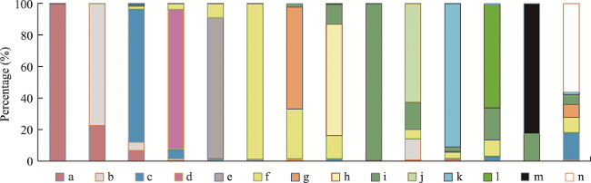
Figure 11 Changes in each land system class from 2017 to other classes in 2030 by proportion (a. Compact city; b. Scattered city; c. Urban-rural fringe; d. Compact town; e. Scattered town; f. Heavily utilized agricultural land; g. Moderately utilized agricultural land; h. Underutilized agricultural land; i. Forest; j. Grasslands; k. Water; l. Mixed; m. Barren land; n. Unclassified land)
It is important to note that the government land-use strategy can be improved according to our analysis. Specifically, the government can adopt a food-production perspective, wherein the focus is placed on whether food production—rather than the area of cropland—remains stable or not. This perspective is more in line with the need to ensure food security, and it has two clear advantages according to our simulation. First, it is easier to implement in terms of agricultural intensification. For example, as shown in Figure 10(f-g), S12 needs less heavily utilized agricultural land than S06. Second, and more importantly, this perspective brings about more ecological benefits. As shown in Figure 10(i), the increase in the environmental class of the land system will increase in area by 5% under S12 compared to only 2% under S06.
To facilitate the adoption of a food-production perspective, the government of Henan should give priority to the evaluation of land-use intensity, especially agricultural intensity. In this study, the agricultural intensity was evaluated in terms of investigated grain production and at the county level due to data availability. However, the agricultural intensity can be better assessed by considering more factors, such as the theoretical maximum production (Ye et al., 2020). In addition, we suggest that the actual grain production is investigated and reported at the local level (e.g., each hectare of cropland).
In conclusion, the modeling results of these scenarios provide a solid basis for making decisions regarding Henan’s urban-rural development. We also revealed the influence mechanism of each population projection, each land-use policy, and each combination, highlighting the benefits of securing food production by agricultural intensification rather than merely expanding the area of cropland. However, one limitation of this study lies in the classification scheme developed for establishing the land system of Henan. As explained in Section 3.2, the scheme consists of 16 land classes designed for exploring detailed urban-rural development under intersecting population growth and food production scenarios. The scheme also contains a set of threshold-based rules, as shown in Figure 2, but the threshold determination was subject to expert experience. Future research is thus recommended to test the universality of these thresholds and to investigate the effects of different thresholds on the simulation of a land system. Future research is also recommended in the following three areas. The first is to determine the future demand for land system services by considering China’s new carbon neutrality pledge. This consideration may be implemented using integrated assessment models such as the Global Change Assessment Model, the Integrated Model to Access the Global Environment, and the Global Biosphere Management Model (e.g., Li et al., 2017; Dong et al., 2018). The second is to consider the temporal variation of the capability of each land class to provide different land system services in the period of simulation. The third is to understand land system dynamics based on thermodynamic insights and Boltzmann (thermodynamic) entropy (e.g., Cushman, 2015, 2016; Gao et al., 2018; Gao and Li, 2019).

Appendix A: Detailed land system simulated for the Henan of 2030 under each scenario

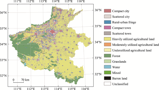
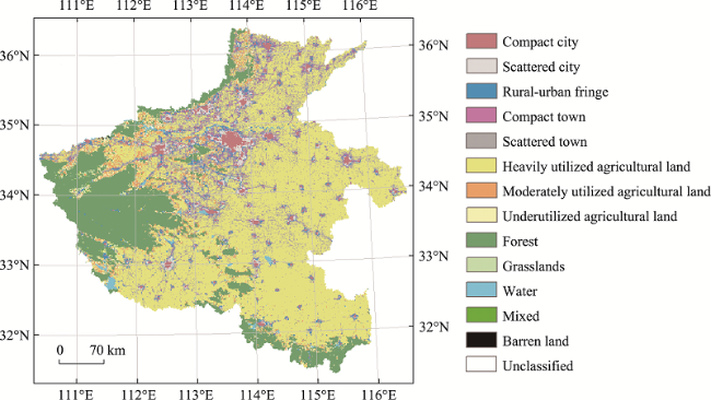
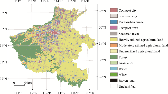
Figure B.1 Simulation under S01
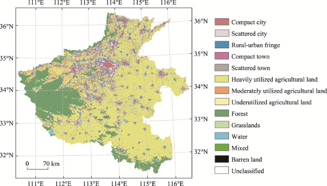
Figure B.2 Simulation under S02
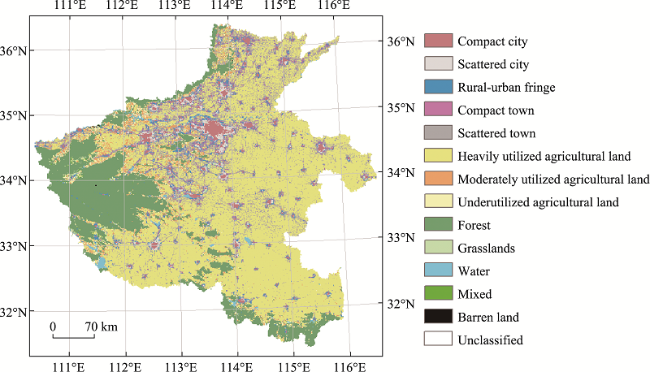
Figure B.3 Simulation under S03
Figure B.4 Simulation under S04
Figure B.5 Simulation under S05
Figure B.6 Simulation under S06
Figure B.7 Simulation under S07
Figure B.8 Simulation under S08
Figure B.9 Simulation under S09
Figure B.10 Simulation under S10
Figure B.11 Simulation under S11
Figure B.12 Simulation under S12
Figure B.13 Simulation under S13
Figure B.14 Simulation under S14
Figure B.15 Simulation under S15
Figure B.16 Simulation under S16
Figure B.17 Simulation under S17
Figure B.18 Simulation under S18

Appendix B: Two sets of standard deviations (SD) calculated for each land system class

One set (SD by row) is calculated by using the land-use policy as the control variable, and the other set (SD by column) is calculated by using the population projection as the control variable.
Table C.1 Standard deviations calculated for compact city
SSP1 SSP2 SSP3 SSP4 SSP5 Planed SD by row
P1 38.26% 41.61% 47.59% 36.11% 37.49% 36.14% 4.43%
P2 38.22% 41.47% 47.81% 35.96% 37.35% 36.07% 4.55%
P3 35.49% 38.95% 45.04% 33.08% 34.61% 33.19% 4.60%
SD by column 1.59% 1.50% 1.54% 1.71% 1.62% 1.68% -
Table C.2 Standard deviations calculated for scattered city
SSP1 SSP2 SSP3 SSP4 SSP5 Planed SD by row
P1 -3.17% 1.90% 14.87% -5.96% -4.03% -5.78% 7.99%
P2 -3.02% 2.57% 16.40% -6.04% -3.88% -5.85% 8.61%
P3 -9.50% -5.40% 2.27% -11.41% -10.21% -11.41% 5.32%
SD by column 3.70% 4.42% 7.75% 3.12% 3.62% 3.23% -
Table C.3 Standard deviations calculated for rural-urban fringe
SSP1 SSP2 SSP3 SSP4 SSP5 Planed SD by row
P1 2.15% 5.70% 18.37% 0.37% 1.11% 0.51% 6.98%
P2 0.77% 4.74% 18.75% -0.81% 0.14% -0.59% 7.58%
P3 -0.12% 2.03% 8.58% -0.69% -0.30% -0.57% 3.62%
SD by column 1.14% 1.90% 5.76% 0.65% 0.72% 0.63% -
Table C.4 Standard deviations calculated for compact town
SSP1 SSP2 SSP3 SSP4 SSP5 Planed SD by row
P1 -11.02% -13.45% -21.22% -9.63% -10.35% -9.61% 4.48%
P2 -10.98% -14.27% -24.39% -9.30% -10.32% -9.28% 5.83%
P3 -10.32% -13.26% -20.46% -9.02% -9.82% -8.83% 4.47%
SD by column 0.40% 0.54% 2.09% 0.31% 0.30% 0.39% -
Table C.5 Standard deviations calculated for scattered town
SSP1 SSP2 SSP3 SSP4 SSP5 Planed SD by row
P1 -5.83% -4.81% -3.78% -6.41% -6.08% -5.70% 0.97%
P2 -1.24% -0.39% 0.60% -1.87% -1.48% -1.33% 0.90%
P3 -5.24% -2.84% 0.26% -6.54% -5.78% -5.88% 2.59%
SD by column 2.49% 2.21% 2.43% 2.66% 2.57% 2.57% -
Table C.6 Standard deviations calculated for heavily-utilized agricultural land
SSP1 SSP2 SSP3 SSP4 SSP5 Planed SD by row
P1 6.13% 6.06% 6.10% 6.21% 6.14% 6.07% 0.06%
P2 3.00% 2.87% 2.69% 3.14% 3.06% 3.03% 0.16%
P3 12.43% 12.47% 12.51% 12.26% 12.41% 12.11% 0.15%
SD by column 4.80% 4.89% 4.99% 4.64% 4.77% 4.62% -
Table C.7 Standard deviations calculated for moderately-utilized agricultural land
SSP1 SSP2 SSP3 SSP4 SSP5 Planed SD by row
P1 -36.05% -38.55% -44.39% -34.83% -35.35% -35.03% 3.70%
P2 -27.01% -29.20% -34.42% -26.22% -26.76% -26.31% 3.18%
P3 -54.88% -55.97% -57.26% -53.87% -54.56% -53.87% 1.33%
SD by column 14.22% 13.59% 11.45% 14.15% 14.23% 14.08% -
Table C.8 Standard deviations calculated for underutilized agricultural land
SSP1 SSP2 SSP3 SSP4 SSP5 Planed SD by row
P1 -30.00% -31.79% -36.60% -29.25% -29.72% -29.20% 2.86%
P2 -32.51% -33.72% -37.67% -31.76% -32.28% -31.48% 2.31%
P3 -58.51% -64.52% -73.17% -54.30% -57.29% -54.22% 7.33%
SD by column 15.79% 18.36% 20.81% 13.79% 15.23% 13.83% -
Table C.9 Standard deviations calculated for the land system class of environment
SSP1 SSP2 SSP3 SSP4 SSP5 Planed SD by row
P1 2.11% 1.80% 1.27% 2.25% 2.17% 2.15% 0.37%
P2 5.45% 5.23% 5.00% 5.53% 5.47% 5.38% 0.20%
P3 -2.45% -3.04% -4.01% -2.11% -2.33% -2.22% 0.72%
SD by column 3.97% 4.16% 4.53% 3.83% 3.92% 3.81% -
[1]
Ahmed S J, Bramley G, Verburg P H, 2014. Key driving factors influencing urban growth:Spatial-statistical modelling with CLUE-S. Dhaka Megacity. Springer.

[2]
Bai Y, Wong C, Jiang B et al., 2018. Developing China’s Ecological Redline Policy using ecosystem services assessments for land use planning. Nature Communications, 9(1): 3034.

DOI

[3]
Bajracharya P, Lippitt C D, Sultana S, 2020. Modeling urban growth and land cover change in Albuquerque using SLEUTH. The Professional Geographer, 72(2): 181-193.

DOI

[4]
Chaudhuri G, Clarke K C, 2019. Modeling an Indian megalopolis: A case study on adapting SLEUTH urban growth model. Computers, Environment and Urban Systems, 77: 101358-101358.

DOI

[5]
Chen Y, Guo F, Wang J et al., 2020. Provincial and gridded population projection for China under shared socioeconomic pathways from 2010 to 2100. Scientific Data, 7(1): 1-13.

DOI

[6]
Cushman S A, 2015. Thermodynamics in landscape ecology: The importance of integrating measurement and modeling of landscape entropy. Landscape Ecology, 30(1): 7-10.

DOI

[7]
Cushman S A, 2016. Calculating the configurational entropy of a landscape mosaic. Landscape Ecology, 31(3): 481-489.

DOI

[8]
Dai K, Shen S, Cheng C et al., 2020. Trade-off relationship of arable and ecological land in urban growth when altering urban form: A case study of Shenzhen, China. Sustainability, 12(23): 10041.

DOI

[9]
Debonne N, van Vliet J, Heinimann A et al., 2018. Representing large-scale land acquisitions in land use change scenarios for the Lao PDR. Regional Environmental Change, 18(6): 1857-1869.

DOI PMID

[10]
Debonne N, van Vliet J, Verburg P H, 2019. Future governance options for large-scale land acquisition in Cambodia: Impacts on tree cover and tiger landscapes. Environmental Science & Policy, 94: 9-19.

[11]
Delzeit R, Zabel F, Meyer C et al., 2017. Addressing future trade-offs between biodiversity and cropland expansion to improve food security. Regional Environmental Change, 17(5): 1429-1441.

DOI

[12]
Deng Y, Liu S, Cai J et al., 2015. Spatial pattern and its evolution of Chinese provincial population: Methods and empirical study. Journal of Geographical Sciences, 25(12): 1507-1520.

DOI

[13]
Dong N, You L, Cai W et al., 2018. Land use projections in China under global socioeconomic and emission scenarios: Utilizing a scenario-based land-use change assessment framework. Global Environmental Change, 50: 164-177.

DOI

[14]
Eitelberg D A, van Vliet J, Doelman J C et al., 2016. Demand for biodiversity protection and carbon storage as drivers of global land change scenarios. Global Environmental Change, 40: 101-111.

DOI

[15]
Ellis E C, Pascual U, Mertz O, 2019. Ecosystem services and nature’s contribution to people: Negotiating diverse values and trade-offs in land systems. Current Opinion in Environmental Sustainability, 38: 86-94.

DOI

[16]
Freire S, Doxsey-Whitfield E, MacManus K et al., 2016. Development of new open and free multi-temporal global population grids at 250 m resolution.

[17]
Gao L, Bryan B A, 2017. Finding pathways to national-scale land-sector sustainability. Nature, 544(7649): 217-222.

DOI

[18]
Gao P, Cushman S A, Liu G et al., 2019. FracL: A tool for characterizing the fractality of landscape gradients from a new perspective. ISPRS International Journal of Geo-Information, 8(10): 466.

DOI

[19]
Gao P, Li Z, 2019. Computation of the Boltzmann entropy of a landscape: A review and a generalization. Landscape Ecology, 34(9): 2183-2196.

DOI

[20]
Gao P, Li Z, Zhang H, 2018. Thermodynamics-based evaluation of various improved Shannon entropies for configurational information of gray-level images. Entropy, 20(1): 19.

DOI

[21]
Gao P, Wang H, Cushman S A et al., 2021a. Sustainable land-use optimization using NSGA-II: Theoretical and experimental comparisons of improved algorithms. Landscape Ecology, 36(7): 1877-1892.

DOI

[22]
Gao P, Zhang H, Li Z, 2017. A hierarchy-based solution to calculate the configurational entropy of landscape gradients. Landscape Ecology, 32(6): 1133-1146.

[23]
Gao P, Zhang H, Wu Z et al., 2021b. A joint landscape metric and error image approach to unsupervised band selection for hyperspectral image classification. IEEE Geoscience and Remote Sensing Letters: 1-5.

[24]
Gong P, Liu H, Zhang M et al., 2019. Stable classification with limited sample: Transferring a 30-m resolution sample set collected in 2015 to mapping 10-m resolution global land cover in 2017. Science Bulletin, 64(6): 370-373.

DOI PMID

[25]
Gong P, Wang J, Yu L et al., 2013. Finer resolution observation and monitoring of global land cover: First mapping results with Landsat TM and ETM+ data. International Journal of Remote Sensing, 34(7): 2607-2654.

DOI

[26]
Government of Henan, 2017. Population Plan of Henan Province (2016-2030). Available from https://www.henan.gov.cn/2017/05-25/248952.html accessed.

[27]
Grundy M J, Bryan B A, Nolan M et al., 2016. Scenarios for Australian agricultural production and land use to 2050. Agricultural Systems, 142: 70-83.

DOI

[28]
He C, Li J, Zhang X et al., 2017. Will rapid urban expansion in the drylands of northern China continue: A scenario analysis based on the land use scenario dynamics-urban model and the shared socioeconomic pathways. Journal of Cleaner Production, 165: 57-69.

DOI

[29]
Henan Bureau of Statistics(HBS), 2018. Henan Statistical Yearbook. Beijing: China Statistics Press.

[30]
Hengl T, de Jesus J M, Heuvelink G B et al., 2017. SoilGrids250m: Global gridded soil information based on machine learning. PLoS One, 12(2): e0169748.

DOI

[31]
Jin G, Deng X, Zhao X et al., 2018. Spatiotemporal patterns in urbanization efficiency within the Yangtze River Economic Belt between 2005 and 2014. Journal of Geographical Sciences, 28(8): 1113-1126.

DOI

[32]
Jin G, Shi X, He D et al., 2020. Designing a spatial pattern to rebalance the orientation of development and protection in Wuhan. Journal of Geographical Sciences, 30(4): 569-582.

DOI

[33]
Kirch P V, Hartshorn A S, Chadwick O A et al., 2004. Environment, agriculture, and settlement patterns in a marginal Polynesian landscape. Proceedings of the National Academy of Sciences, 101(26): 9936-9941.

DOI

[34]
Kuang W, 2019. Mapping global impervious surface area and green space within urban environments. Science China Earth Sciences, 62(10): 1591-1606.

DOI

[35]
Kuang W, Dou Y, 2020. Investigating the patterns and dynamics of urban green space in China’s 70 major cities using satellite remote sensing. Remote Sensing, 12(12): 1929.

DOI

[36]
Lan T, Li Z, Ti P, 2019. Integrating general principles into mixed-integer programming to optimize schematic network maps. International Journal of Geographical Information Science, 33(11): 2305-2333.

DOI

[37]
Li X, Chen G, Liu X et al., 2017. A new global land-use and land-cover change product at a 1-km resolution for 2010 to 2100 based on human-environment interactions. Annals of the American Association of Geographers, 107(5): 1040-1059.

DOI

[38]
Li X, Chen Y, 2020. Projecting the future impacts of China’s cropland balance policy on ecosystem services under the shared socioeconomic pathways. Journal of Cleaner Production, 250: 119489.

DOI

[39]
Liao W, Liu X, Xu X et al., 2020. Projections of land use changes under the plant functional type classification in different SSP-RCP scenarios in China. Science Bulletin, 65(22): 1935-1947.

DOI PMID

[40]
Liu X, Liang X, Li X et al., 2017. A future land use simulation model (FLUS) for simulating multiple land use scenarios by coupling human and natural effects. Landscape and Urban Planning, 168: 94-116.

DOI

[41]
Liu Y, Wang J, Long H, 2010. Analysis of arable land loss and its impact on rural sustainability in Southern Jiangsu Province of China. Journal of Environmental Management, 91(3): 646-653.

DOI PMID

[42]
Long H, Liu Y, Wu X et al., 2009. Spatio-temporal dynamic patterns of farmland and rural settlements in Su-Xi-Chang region: Implications for building a new countryside in coastal China. Land Use Policy, 26(2): 322-333.

DOI

[43]
Lu Y, Chen B, 2017. Urban ecological footprint prediction based on the Markov chain. Journal of Cleaner Production, 163: 146-153.

DOI

[44]
Ma Y, Cheng J, Jiao F et al., 2008. Distribution, sources, and potential risk of polycyclic aromatic hydrocarbons (PAHs) in drinking water resources from Henan Province in middle of China. Environmental Monitoring and Assessment, 146(1-3): 127-138.

DOI

[45]
McGarigal K, Cushman S A, 2005. The gradient concept of landscape structure. In: Wiens J A, Moss M R (eds). Issues and Perspectives in Landscape Ecology. Cambridge‎: Cambridge University Press.

[46]
National Bureau of Statistics of China(NBSC), 2019a. Announcement of Statistics on Grain Production. Available from http://www.stats.gov.cn/tjsj/zxfb/201912/t20191206_1715827.html accessed 15 Oct. 2021.

[47]
National Bureau of Statistics of China (NBSC), 2019b. China Statistical Yearbook. Beijing: China Statistics Press.

[48]
O’Neill B C, Kriegler E, Riahi K et al., 2014. A new scenario framework for climate change research: The concept of shared socioeconomic pathways. Climatic Change, 122(3): 387-400.

DOI

[49]
Peng J, Hu X, Wang X et al., 2019a. Simulating the impact of Grain-for-Green Programme on ecosystem services trade-offs in northwestern Yunnan, China. Ecosystem Services, 39: 100998.

DOI

[50]
Peng J, Liu Q, Blaschke T et al., 2020. Integrating land development size, pattern, and density to identify urban-rural fringe in a metropolitan region. Landscape Ecology, 35(9): 2045-2059.

DOI

[51]
Peng J, Wang A, Luo L et al., 2019b. Spatial identification of conservation priority areas for urban ecological land: An approach based on water ecosystem services. Land Degradation & Development, 30(6): 683-694.

DOI

[52]
Peng S, Ding Y, Liu W et al., 2019c. 1 km monthly temperature and precipitation dataset for China from 1901 to 2017. Earth System Science Data, 11(4).

[53]
Pesaresi M, Huadong G, Blaes X et al., 2013. A global human settlement layer from optical HR/VHR RS data: Concept and first results. IEEE Journal of Selected Topics in Applied Earth Observations and Remote Sensing, 6(5): 2102-2131.

DOI

[54]
Pouzols F M, Toivonen T, Di Minin E et al., 2014. Global protected area expansion is compromised by projected land-use and parochialism. Nature, 516(7531): 383-386.

DOI

[55]
Riahi K, Van Vuuren D P, Kriegler E et al., 2017. The shared socioeconomic pathways and their energy, land use, and greenhouse gas emissions implications: An overview. Global Environmental Change, 42: 153-168.

DOI

[56]
Sahoo S, Sil I, Dhar A et al., 2018. Future scenarios of land-use suitability modeling for agricultural sustainability in a river basin. Journal of Cleaner Production, 205: 313-328.

DOI

[57]
Shaker R R, Altman Y, Deng C et al., 2019. Investigating urban heat island through spatial analysis of New York City streetscapes. Journal of Cleaner Production, 233: 972-992.

[58]
Sun X, Lu Z, Li F et al., 2018. Analyzing spatio-temporal changes and trade-offs to support the supply of multiple ecosystem services in Beijing, China. Ecological Indicators, 94: 117-129.

DOI

[59]
Talukdar S, Pal S, 2020. Modeling flood plain wetland transformation in consequences of flow alteration in Punarbhaba River in India and Bangladesh. Journal of Cleaner Production, 261: 120767.

DOI

[60]
Tang S, Zhang L, Hao Y et al., 2021. System dynamics modeling for construction material flows of urban residential building: A case study of Beijing, China. Resources, Conservation and Recycling, 168: 105298.

DOI

[61]
van Vliet J, Eitelberg D A, Verburg P H, 2017. A global analysis of land take in cropland areas and production displacement from urbanization. Global Environmental Change, 43: 107-115.

DOI

[62]
van Vliet J, Verburg P H, 2018. A short presentation of CLUMondo. In: Camacho Olmedo M T, Paegelow M, Mas J-F et al. eds. Geomatic Approaches for Modeling Land Change Scenarios. Springer International Publishing, Cham.

[63]
Vasenev V I, Stoorvogel J J, Leemans R et al., 2018. Projection of urban expansion and related changes in soil carbon stocks in the Moscow Region. Journal of Cleaner Production, 170: 902-914.

DOI

[64]
Verburg P H, Soepboer W, Veldkamp A et al., 2002. Modeling the spatial dynamics of regional land use: The CLUE-S model. Environmental Management, 30(3): 391-405.

PMID

[65]
Wallace K J, 2007. Classification of ecosystem services: Problems and solutions. Biological Conservation, 139(3/4): 235-246.

DOI

[66]
Wang T, Kazak J, Han Q et al., 2019a. A framework for path-dependent industrial land transition analysis using vector data. European Planning Studies, 27(7): 1391-1412.

DOI

[67]
Wang Y, van Vliet J, Pu L et al., 2019b. Modeling different urban change trajectories and their trade-offs with food production in Jiangsu Province, China. Computers, Environment and Urban Systems, 77: 101355.

[68]
Weiss D J, Nelson A, Gibson H S et al., 2018. A global map of travel time to cities to assess inequalities in accessibility in 2015. Nature, 553(7688): 333-336.

DOI

[69]
Wolff S, Schrammeijer E A, Schulp C J et al., 2018. Meeting global land restoration and protection targets:What would the world look like in 2050? Global Environmental Change, 52: 259-272.

[70]
Ye S, Song C, Shen S et al., 2020. Spatial pattern of arable land-use intensity in China. Land Use Policy, 99: 104845.

DOI

[71]
Zhang H, Wu Z, Lan T et al., 2020. Calculating the Wasserstein metric-based Boltzmann entropy of a landscape mosaic. Entropy, 22(4): 381.

DOI

[72]
Zhu W, Zhang J, Cui Y et al., 2020. Ecosystem carbon storage under different scenarios of land use change in Qihe catchment, China. Journal of Geographical Sciences, 30(9): 1507-1522.

DOI

[73]
Zou L, Liu Y, Wang J et al., 2019. Land use conflict identification and sustainable development scenario simulation on China’s southeast coast. Journal of Cleaner Production, 238: 117899.

DOI

Outlines

/