Extraction and spatiotemporal evolution analysis of tidal flats in the Bohai Rim during 1984-2019 based on remote sensing

  • XU Haijue , 1, 2 ,
  • JIA Ao 1 ,
  • SONG Xiaolong 1, 2 ,
  • BAI Yuchuan 1, 2
Expand
  • 1. State Key Laboratory of Hydraulic Engineering Simulation and Safety, Tianjin University, Tianjin 300350, China
  • 2. Institute for Sedimentation on River and Coastal Engineering, Tianjin University, Tianjin 300350, China
*Song Xiaolong, Lecturer, E-mail:

Xu Haijue, Associate Professor, E-mail:

Received date: 2021-11-24

  Accepted date: 2022-06-02

  Online published: 2023-01-16

Supported by

National Key Research and Development Program of China(2018YFC0407505)

National Natural Science Foundation of China(51879182)

Science and Technology Planning Program of Tianjin, China(21JCQNJC00480)

Copyright

© 2023

Abstract

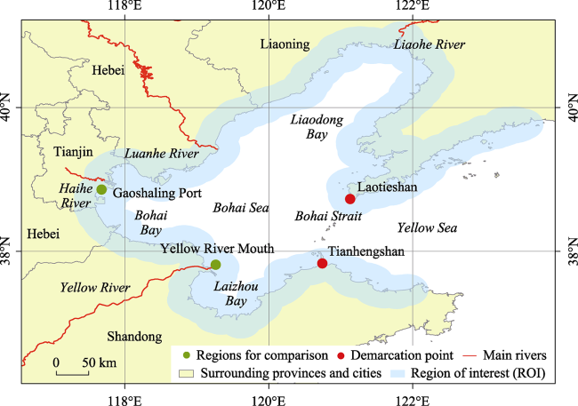
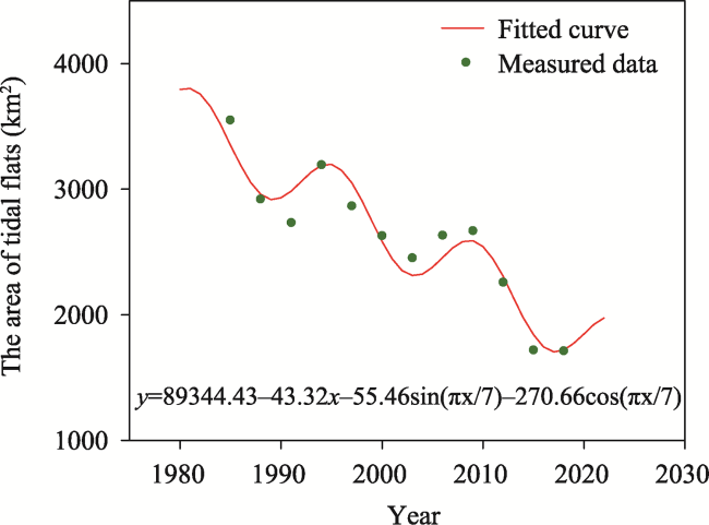
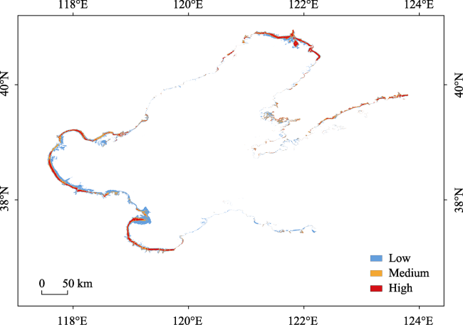
Tidal flats, a precious resource that provides ecological services and land space for coastal zones, are facing threats from human activities and climate change. In this study, a robust decision tree for tidal flat extraction was developed to analyse spatiotemporal variations in the Bohai Rim region during 1984-2019 based on 9539 Landsat TM/OLI surface reflection images and the Google Earth Engine (GEE) cloud platform. The area of tidal flats significantly fluctuated downwards from 3551.22 to 1712.36 km2 in the Bohai Rim region during 1984-2019, and 51.31% of tidal flats were distributed near the Yellow River Delta and Liaohe River Delta during 2017-2019. There occurred a drastic spatial transition of tidal flats with coastline migration towards the ocean. Low-stability tidal flats were mainly distributed in reclamation regions, deltas, and bays near the estuary during 1984-2019. The main factors of tidal flat evolution in the Bohai Rim region included the direct impact of land cover changes in reclamation regions, the continuous impact of a weakening sediment supply, and the potential impact of a deteriorating sediment storage capability. The extraction process and maps herein could provide a reference for the sustainable development and conservation of coastal resources.

Cite this article

XU Haijue , JIA Ao , SONG Xiaolong , BAI Yuchuan . Extraction and spatiotemporal evolution analysis of tidal flats in the Bohai Rim during 1984-2019 based on remote sensing[J]. Journal of Geographical Sciences, 2023 , 33(1) : 76 -98 . DOI: 10.1007/s11442-023-2075-0

1 Introduction

Tidal flats usually include muddy, sandy, or bedrock bare land areas between high- and low-water lines where the water level greatly fluctuates affected by tidal currents, waves, or precipitation (Yan et al., 2011; Wang et al., 2018; Murray et al., 2019). Tidal flats play key roles not only in providing land resources for urban development but also in protecting biodiversity, degrading environmental pollutants, and buffering storm surges (Polte et al., 2005; Temmerman et al., 2013; Chen et al., 2016; Ghosh et al., 2016; Sagar et al., 2017; Zhang et al., 2019). However, a significant downward trend in the tidal flat area at both regional and global scales was reported (Wang et al., 2018; Murray et al., 2019), combined with continuous natural and human factors in the fragile intertidal zone, such as sea-level rise (Luo et al., 2011; Passeri et al., 2015), land subsidence (Xue et al., 2005; Zhang et al., 2015), reclamation (Robert et al., 2007; Ding et al., 2019) and reduction in the river sediment supply (Blum and Roberts, 2009; Ren et al., 2015). It is thus necessary to monitor the distribution and explore the spatiotemporal evolution characteristics of coastal tidal flats for scientific protection and development purposes.
Satellite remote sensing has become a more efficient tidal flat surveying method on large scales than the ground surveying, underwater topographic surveying, and airborne remote sensing methods (Mason et al., 2010). This method has also been widely used in the detection of water resources (Zou et al., 2017, 2018) and forest resources (Hansen et al., 2013; Yu et al., 2018) at a high efficiency. With open access to high-resolution and long time series remote sensing images, e.g., Landsat data (Masek et al., 2020), and powerful parallel processing capabilities provided by the Google Earth Engine (GEE) cloud platform (Kumar and Mutanga, 2018; Huang et al., 2021), it is highly convenient to monitor land cover with a high resolution at regional, continental or planetary scales. In addition, there are fewer open-access datasets for tidal flats, as these areas are traditionally recognized as part of wetlands in most land cover data, e.g., MODIS annual land cover classification data (MCD12Q1) (Friedl et al., 2002) or the GlobeLand30 dataset (Chen et al., 2014). It is necessary to continuously monitor tidal flats with a simple but quick and robust algorithm to ensure the timeliness and continuity of monitoring data based on satellite remote sensing (Wang et al., 2018; Jia et al., 2021).
The waterline and its trajectory were originally used to simulate the range of tidal flats. Murray et al. (2012) mapped tidal flats across East Asia by extracting submerged areas at high and low tides and subsequently subtracting the submerged regions at low tides from those at high tides. Liu et al. (2016) analysed high- and low-tide sets of automatically generated waterlines to identify tidal flats with the Digital Shoreline Analysis System (DSAS) and Jenks natural breaks algorithm in the Bohai Rim region. Chen et al. (2016) obtained the intertidal zone range in the Yangtze River estuary through artificial highest-tide shorelines and automatic lowest-tide shorelines based on water frequency maps. Han et al. (2018) calculated the intertidal zone range based on instant waterline, tide, and topographic data. Most of these methods required images with a low cloud cover or additional supporting data, e.g., tide and topographic data, for the study area, while the temporal characteristics of remote sensing images were not fully considered. In addition, supervised classification, especially the random forest model, was employed to extract the range of tidal flats via land cover classification based on image features. Murray et al. (2019) extracted the global tidal flat distribution during 1984-2016 based on the random forest classification method and the statistical characteristics of Landsat image sequences. Zhang et al. (2019) analysed tidal flats in the intertidal zone and vegetation in the supra-zone along the coast from Hangzhou Bay to the Bohai Sea based on the random forest classification method, statistical characteristics of Landsat image series, and object-based post-processing method. These methods considered the statistical characteristics of time series images. However, these methods are costly, time consuming, and highly dependent on training data.
In recent years, decision trees based on the statistical characteristics of an image sequence have been reported as a highly efficient method in the automatic tracking of tidal flats. Sagar et al. (2017) estimated the intertidal extent in Australia based on median composite images of the normalized difference water index (NDWI). Wang et al. (2018) extracted the annual distribution of tidal flats along the coast of China from 1984 to 2016 based on the water frequency, in which the water distribution was extracted by a decision tree, as proposed by Zou et al. (2017), with the modified normalized difference water index (MNDWI), normalized difference vegetation index (NDVI) and enhanced vegetation index (EVI). Jia et al. (2021) developed a workflow by integrating the maximum spectral index composite values based on the MNDWI and NDVI and subsequently extracting the maximal and minimal water extents with the Otsu threshold methods. These decision trees were repeatable and feasible for surface water or tidal flat extraction, among which the MNDWI and NDWI were commonly used. The NDVI and EVI were introduced as an inverse indicator or dynamic threshold to reduce the turbulence in vegetation in response to water to delimit pixels containing water and vegetation (Zou et al., 2017, 2018; Wang et al., 2018; He et al., 2020). However, due to the different bands used in the establishment of water indices, they reflected different boundaries of the surface water (Donchyts et al., 2016; Sagar et al., 2017), and this difference was less notably considered in the above studies.
The coastal area surrounding the Bohai Rim is a typical region affected by intense human activities with abundant tidal flat resources. In this study, a decision tree was developed to map the distribution and analyse the spatiotemporal evolution characteristics of tidal flats in the Bohai Rim region from 1984 to 2019 based on the difference in the MNDWI and NDWI of Landsat TM/OLI surface reflection image sequences and the GEE cloud platform. Specifically, we 1) developed a simple and robust decision tree algorithm for tidal flat extraction, 2) analysed the distribution and evolution characteristics of tidal flats and coastlines, and 3) preliminarily studied the impacts of three factors on the evolution of tidal flats in the Bohai Rim region.

2 Data and methodology

2.1 Study area

The Bohai Sea (Figure 1) is a part of the Western Pacific Ocean and a semi-enclosed sea in northern China, situated from 37°07'N to 41°00'N and 117°35'E to 121°00'E. This area comprises three bays, including Liaodong Bay, Bohai Bay, and Laizhou Bay, and is enclosed by three provinces (Liaoning, Hebei and Shandong) and one municipality (Tianjin) in counter-clockwise order. The Bohai Sea and Yellow Sea are connected through the Bohai Strait and divided by a straight line between the two capes at Laotieshan (north) and Tianhengshan (south), respectively. As tidal flats are usually distributed within a narrow coastal region (Murray et al., 2019), a buffer zone of 25 km extending to both the land and sea from the coastal administrative boundaries of thirteen cities around the Bohai Sea was selected as the region of interest (ROI), covering an area of approximately 92,000 km2.
Figure 1 Location of the study area (Bohai Rim region)

2.2 Data acquisition

Geometrically corrected (L1T) surface reflectance data of Landsat TM 5 (LT05) and Landsat OLI 8 (LC08) from 1984/01/01 to 2019/12/31 provided on the GEE cloud platform were used for tidal flat detection and shoreline extraction. These images were subjected to radiometric calibration and atmospheric correction, totalling 9539 available images intersecting with the ROI.
The monthly average sea level in August in the Bohai Sea during 1980-2019 was acquired from the China Oceanic Information Network (http://www.nmdis.org.cn). Affected by local runoff and precipitation, there usually occurred a higher sea level in August and a larger influence region. Annual data of the runoff and sediment load of the Yellow River from 1984 to 2018 were collected at Lijin Station, the gauging station on the Yellow River closest to the estuary, to analyse the impact of the sediment supply on the erosion and expansion processes of tidal flats in the Yellow River Delta.

2.3 Algorithm to extract tidal flats in the coastal zone

The land cover in the intertidal zone could be divided into coastal vegetation and tidal flats (Figure 2) (Wang et al., 2018; Murray et al., 2019). Coastal vegetation, including mangroves at lower latitudes and saltmarshes at higher latitudes, often occurs in supra-tidal or upper intertidal zones (Chen et al., 2021; Fu et al., 2021) and can be distinguished from bare tidal flats (Wang et al., 2018; Zhang et al., 2019). Tidal zones with vegetation growth provide the same important ecological functions as do tidal flats, and these zones are usually developed together, as both types are located in not only the same geomorphological units but also in the immediate area. These vegetation flats remain relatively stable under ocean dynamics (Temmerman et al., 2013), and their evolution is usually determined by the expansion of the distribution range of plants adapted to prolonged inundation and increased salinity (Ge et al., 2015). Trace lines, formed between tidal and vegetation flats, are also commonly used to recognize coastlines (Zhang and Niu, 2021). Therefore, bare tidal flats were extracted as a separate category and analysed to explore their buffering effect between water and other coastal land cover areas with a higher stability (including vegetation and other lands) in this research. In addition, to distinguish intertidal and inland tidal flats, e.g., tidal flats in lakes, tidal flats in the affected regions scanned based on the coastlines during twelve periods, buffer region extending 1 km towards both land inside the internal coastline and water outside the external coastline were extracted.
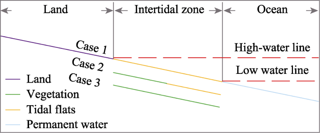
Figure 2 Brief illustration of the land, intertidal zone, and sea areas, modified from Wang et al. (2018). Tidal flats might occupy zero, part, or all of the intertidal zones in some cases.
There were five steps (Figure 3) in the process of tidal flat extraction in this study, including 1) Landsat data pre-processing, 2) surface water identification, 3) land cover classification, 4) object-based post-processing, and 5) accuracy evaluation.
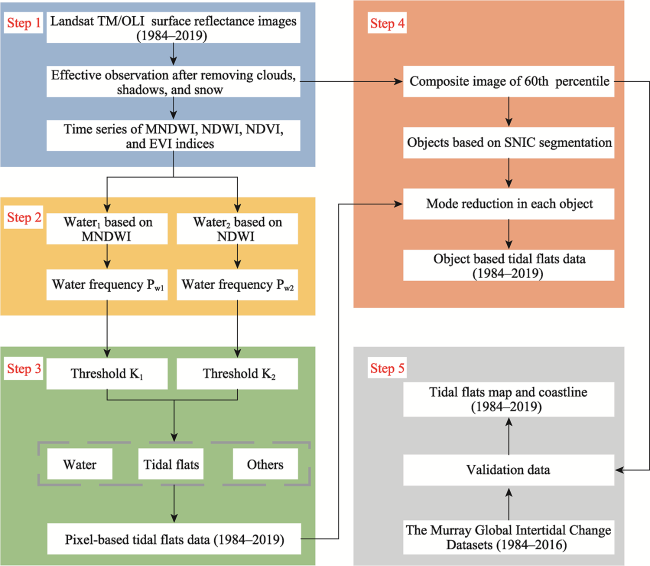
Figure 3 Workflow to extract the tidal flat distribution

2.3.1 Landsat data pre-processing

The pre-processing step mainly included the acquisition of effective observations and the calculation of index bands for the remote sensing image sequences. The quality band generated by the CFMask algorithm (Qiu et al., 2019) was selected to remove clouds, cloud shadows, or snow in images with a cloud cover higher than 3%, and the Simple Cloud Score, a rudimentary cloud scoring algorithm provided by the GEE, was employed to mask bad observations of other images to reduce the effect of misclassification caused by temperature differences, which significantly increased the amount of available data near the seawall.
Water index and vegetation index bands were calculated to highlight water bodies and eliminate the influence of plants, respectively, including the NDWI (McFeeters, 1996), MNDWI (Xu, 2006), NDVI (Tucker, 1979), and EVI (Huete et al., 2002). These four indices can be calculated with Eqs. (1) to (4).
$NDWI=\frac{Green-NIR}{Green+NIR}$
$MNDWI=\frac{Green-SWIR1}{Green+SWIR1}$
$NDVI=\frac{NIR-Red}{NIR+Red}$
$EVI=2.5\times \frac{NIR-Red}{NIR+6\times Red-7.5\times Blue+1}$
where Blue, Green, Red, NIR, and SWIR1 denote the scaled blue (0.45-0.52 μm), green (0.52-0.60 μm), red (0.63-0.69 μm), near-infrared (0.76-0.90 μm), and shortwave infrared 1 (1.55-1.75 μm) surface reflectance values of LT05/LC08, obtained by dividing the original band value 10,000.

2.3.2 Surface water identification

Figure 4 shows the different characteristics of the trend in the water and vegetation indices at equally spaced sample points within a section from land to sea, especially the MNDWI and NDWI. The MNDWI was highly sensitive to water bodies and rose quickly near the boundary between tidal flats and bare land, while the NDWI was highly sensitive to sediments and rapidly increased near the boundary between tidal flats and permanent water bodies. These two boundaries were considered as the traces of high- and low-water levels in a single image, corresponding to two types of decision trees that could divide each pixel into water body and non-water body pixel components. In this study, these two decision trees were established to identify the water body surface as expressed in Eqs. (5) and (6), respectively, in which water1 and water2 denote the water masks extracted by these two decision trees.
$wate{{r}_{1}}=\left\{ \begin{matrix} 1 & MNDWI>NDVI\text{ or }MNDWI>EVI,\text{ }EVI<0.1 \\ 0 & \text{other} \\ \end{matrix} \right.$
$wate{{r}_{2}}\text{ }=\left\{ \begin{matrix} 1 & NDWI>NDVI\text{ or }NDWI>EVI,\text{ }EVI<0 \\ 0 & \text{other} \\ \end{matrix} \right.$
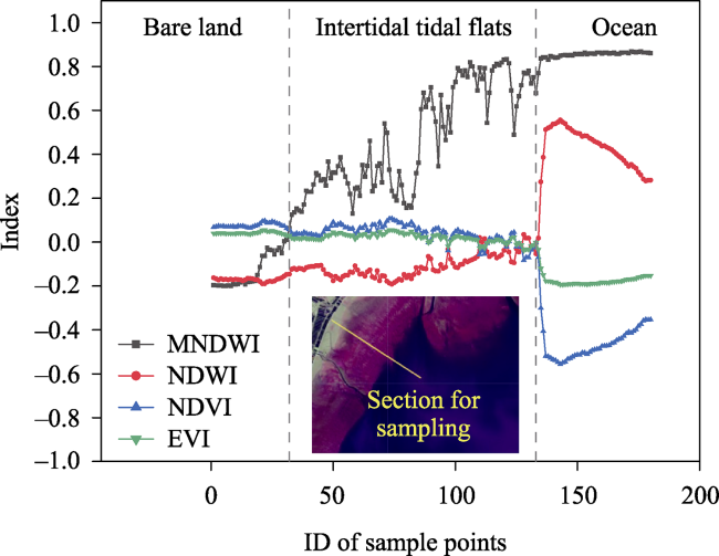
Figure 4 Trend of the water and vegetation indices at equally spaced sample points within a section from land to sea

2.3.3 Land cover classification

Longer image sequences could provide a higher certainty of covering high and low tide levels (Sagar et al., 2017) and seasonal phenological changes (Wang et al., 2018). The 36-month period provided a high stability in tidal flat extraction (Murray et al., 2019; Zhang et al., 2019) and was adopted in this study to reduce the effects of tides and seasonal phenological changes. The methods to calculate two corresponding water frequencies for each pixel and the decision trees established for land cover classification during each period are expressed as Eqs. (7) to (9).
${{P}_{w1}} =\frac{{{n}_{water1}}}{{{n}_{quality}}}$
${{P}_{w2}}\text{ }=\frac{{{n}_{water2}}}{{{n}_{quality}}}$
$Class=\left\{ \begin{matrix} Land \\ Permanent\text{ }water \\ Tidal\text{ }flats \\ \end{matrix}\begin{matrix}, \\, \\, \\ \end{matrix}\begin{matrix} {{P}_{w1}}<{{K}_{1}} \\ {{P}_{w2}}>{{K}_{2}} \\ other \\ \end{matrix} \right.$
where nwater1 and nwater2 are the counts of images wherein the pixels are recognized as surface water with Eqs. (5) and (6), respectively, nquality denotes the count of images wherein the pixels are recognized as effective observations, Pw1 and Pw2 are the two water frequencies corresponding to nwater1 and nwater2, respectively, and K1 and K2 denote the thresholds of the decision tree to identify permanent tidal flats and land, respectively, based on the water frequency.
In previous studies, the range of 0.25-0.75 or 0.05-0.95 were used as thresholds to identify seasonal waters or tidal flats, respectively, based on the annual water frequency (Zou et al., 2017, 2018; Wang et al., 2018; He et al., 2020). Here, we used a longer period and introduced the NDWI to mark trace lines to reflect low-water levels. Figure 5 shows the area trends of land and water for the different thresholds of Pw1 and Pw2, respectively, in the ROI. The areas extracted by K1 or K2 exhibited consistent historical trends from 0.2-0.8, and their corresponding boundaries gradually moved along the vertical direction of the coastline upon thresholds change. Figure 6 shows the distribution of the water frequency of approximately 3600 sample points of the three basic landcover types. K1=0.5 was selected to distinguish land and other land cover types and to extract the average high-tide line. K2=0.8 was selected to monitor lower tidal flats while ensuring consistent results.
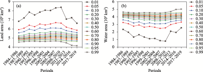
Figure 5 Land and water areas with the different thresholds of Pw1 and Pw2, respectively, in the ROI
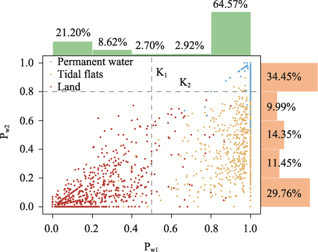
Figure 6 Distribution of the water frequency of approximately 3600 sample points of the three basic landcover types

2.3.4 Object-based post-processing

The object-based method was introduced in the post-processing process, which was suggested to reduce the disturbance due to bad observations and noise in cartography (Ghorbanian et al., 2020). Composite images, calculated via image collection reduction in the 60th percentile (P60) statistic pixel value during each period within each band, were selected to improve the visual difference between tidal flats and other land cover types and generate objects under super-pixel clustering based on the simple non-iterative clustering (SNIC) algorithm (Achanta and Süsstrunk, 2017), with a seed location spacing of eight pixels and connectivity along eight directions.

2.3.5 Accuracy evaluation

The overall accuracy and kappa coefficient based on the confusion matrix (Stehman, 1997) were selected to analyse the classification accuracy and consistency, respectively. The validation data consisted of 3600 manually labelled sample points through P60 composite images for twelve periods during 1984-2019 and 33,000 automatically generated sample points based on randomly generated locations and their corresponding land cover labels obtained through the Murray Global Intertidal Change Datasets (Murray et al., 2019) during 1984-2016 (data were lacking in 2017-2019).

2.4 Shoreline evolution

The upper boundary line of tidal flats during each period was extracted as a coastline, corresponding to the commonly used high-water level line or the average high-tide line (Boak and Turner, 2005). The vertical section method, developed by the U.S. Geological Survey, as the ArcGIS extension module DSAS, has been widely used in the analysis of coastlines and delta evolution (Dada et al., 2016; Shi et al., 2017). The end point rate (EPR) between the coastlines during three periods (1984-1986, 1999-2001, and 2017-2019) was calculated to analyse the characteristics of the erosion and expansion processes surrounding the Bohai Sea.

3 Results and analysis

3.1 Distribution of tidal flats during 1984-2019

The tidal flat distribution in the Bohai Rim region drastically changed and was mainly distributed in the Liaohe Delta, Bohai Bay, Yellow River Delta, and southwestern part of Laizhou Bay, as shown in Figure 7. The area of tidal flats surrounding the Bohai Sea during 2017-2019 reached approximately 1712.36 km2, which dropped by 51.78% from the value of 3551.22 km2 during 1984-1986. Figure 8 shows the areas of tidal flats in thirteen surrounding cities during 1984-1986, 1999-2001, and 2017-2019. Apart from Qinhuangdao, which exhibited a slightly increasing trend, the tidal flat area in the remaining twelve cities exhibited a significant downward trend during 1984-2019. Among these cities, four cities, including Cangzhou, Binzhou, Dongying, and Yantai, attained a reduced reduction rate after the 1999-2001 period, while the other eight cities indicated a higher reduction rate. The tidal flat resources in the Bohai Rim were concentrated in six cities near the Yellow River Delta and Liaohe Delta. The average portion of the tidal flat area and coastline length reached 47.20% and 26.31%, respectively, during the twelve periods. During 2017-2019, the proportion of the tidal flat area (51.31%) was the highest among the twelve periods, while the proportion of the coastline length (25.16%) was the second lowest, and the concentration of the tidal flat spatial distribution (the ratio of the area proportion to the coastline length proportion) continued to increase.
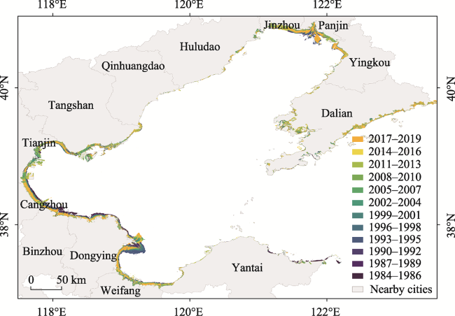
Figure 7 Distribution of tidal flats in the Bohai Rim region in twelve periods during 1984-2019
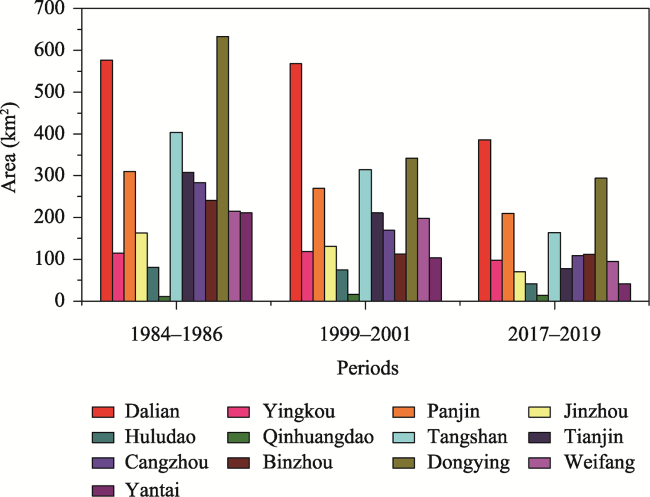
Figure 8 Areas of the tidal flats in thirteen cities in the Bohai Rim region during 1984-1986, 1999-2001, and 2017-2019

3.2 Historical trend of the tidal flat area

The total area of coastal tidal flats in the Bohai Rim region indicated a significant fluctuating downward trend (Figure 9). A combination of trigonometric and linear functions was used to fit these fluctuating and downward trends. The period was assumed as an integer value in years, and the multiple parameters for each part were calculated via the least square method. The function with the smallest error indicated that the period lasted approximately 14 years. Therefore, the 1984-2019 period could be divided into three periods: 1984-1986, 1997-2010, and 2011-2019 (an incomplete cycle). The tidal flat area maintained a downward trend, although there occurred increasing ranges in the fluctuation process. The amplitude and slope of the tidal flat area in the intertidal zone were 276.28 km2 and -43.32 km2/a, respectively, and there existed a smaller influence of the amplitude on the rate of decline than that on the slope.
Figure 9 Historical changes in the intertidal tidal flat area in the Bohai Rim region

3.3 Stability of tidal flats in the Bohai Rim region

The tidal flats in the Bohai Rim region underwent a drastic transition during 1984-2019, especially in the Yellow River Delta, Bohai Bay, and Liaohe River Delta. The total area of the regions where tidal flats once occurred reached approximately 6008.92 km2 during 1984-2019, which far exceeded the areas of tidal flats during any single period. To assess the spatial distribution of the tidal flat stability and identify their transition characteristics in the Bohai Rim region, the stability index for each pixel was measured based on the tidal flat frequency over twelve periods. The higher the frequency of tidal flats, the more stable the tidal flats are. The stability index was equally divided into low (L), medium (M), and high (H) levels corresponding to frequencies of 1-4, 5-8, and 9-12, respectively, as shown in Figure 10. Most of the tidal flats in the Bohai Rim region exhibited a low stability. The low, medium and high levels of the stability index accounted for 51.85%, 23.86%, and 24.29%, respectively, of the total areas. Tidal flats with a low stability index were mainly distributed in deltas and reclamation regions. Among these areas, the tidal flats in deltas, e.g., the Yellow River Delta and Liaohe River Delta, were dominated by natural erosion and siltation, usually accompanied by sandwich structures with the stability gradually decreasing from the inside outwards. These regions, as sensitive coastal land areas, also serve as a potential buffer against hydrodynamic changes. Tidal flats in reclamation regions were closely related to the construction of ports or industrial areas shaped by embankments or other infrastructures, and there occurred few obvious tidal flats formed via natural deposition on the outside of these structures because of the reduced sediment storage capability due to reclamation (Liang et al., 2018).
Figure 10 Stability index of tidal flats in the Bohai Rim region during 1984-2019

3.4 Coastline evolution around the Bohai Sea

The coastline around the Bohai Sea (Figure 11) significantly increased during 1984-2019. In summary, the median year was used to represent each period, i.e., 1985, 2000, and 2018 were selected to represent 1984-1986, 1999-2001, and 2017-2019, respectively. The total length in the ROI increased from 3741 km in 1985 to approximately 4410 km in 2018, at a growth rate of 17.88%. The EPR for 1665 sections of the coastline from the Tianhengshan to Laotieshan Mountains were calculated, as shown in Figures 12 and 13. The coastline around the Bohai Sea significantly shifted towards the ocean, especially after 2000. The average EPR from 2000-2018 was 120.36 m/a, approximately 5 times the rate during 1985-2000. The evolution of the coastline before 2000 was mainly caused by natural delta growth and embankment construction for saltpans or aquafarms in supra-tidal or intertidal zones. The bay with the largest average change was Liaodong Bay before 2000. A rapid increase in reclamation in the intertidal or sub-tidal regions was the main reason for the intensified evolution after 2000, especially port construction in Bohai Bay.
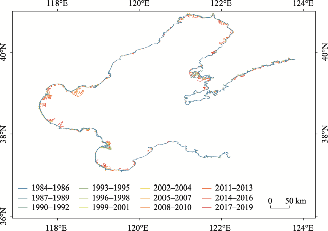
Figure 11 Distribution of coastlines in the Bohai Rim region during twelve periods from 1984 to 2019
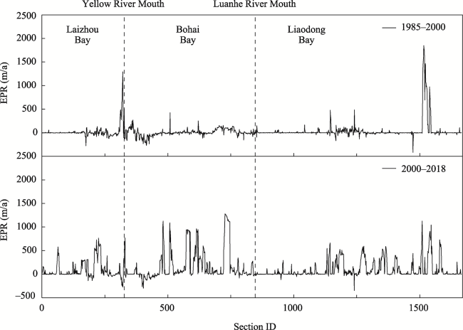
Figure 12 EPR for each section in the Bohai Rim region during 1985 to 2018
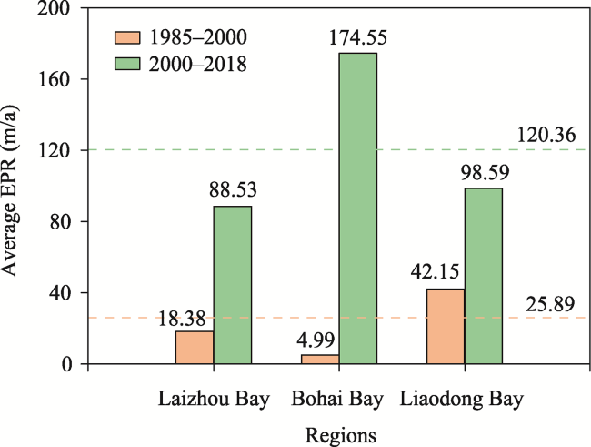
Figure 13 Average EPR for the different sections in each bay in the Bohai Rim region. The dashed line indicates the average EPR for all the sections in the Bohai Rim.

4 Discussion

4.1 Accuracy of tidal flat mapping and comparison to other data

Figure 14 shows the accuracy of tidal flat maps verified via visual interpretation of sample points in P60 composite images during 1984-2019 and random points labelled based on Murray Global Intertidal Change Datasets data (Murray et al., 2019) during 1984-2016, in which the horizontal dashed line indicates the mean or average value. There occurred both a high classification accuracy (overall accuracy > 90% and kappa coefficient > 0.85%) with visual data interpretation and a high consistency with Murray’s study (overall accuracy > 85% and kappa coefficient > 75%).
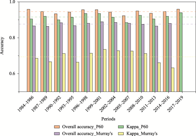
Figure 14 Accuracy of tidal flat maps verified via visual interpretation of sample points in P60 composite images and random points labelled with Murray Global Intertidal Change Datasets data
Comparisons to existing studies were also conducted at three levels, namely, the water detection method, tidal flat distribution, and regional tidal flat area. As shown in Figure 15, six water detection methods commonly used in tidal flat extraction were compared based on the LC08 image with the lowest cloud cover in 2013 at the Yellow River Mouth. Comparison between subfigures a) to c) and subfigures d) to e) revealed the difference in the MNDWI and NDWI between regions with shallow mudflats in which the water surface detected with the MNDWI commonly resulted in higher water lines. In addition, the vegetation index, as a mutable threshold, provided a better performance in reducing the impact of sediment and vegetation conditions than that obtained with a fixed threshold specified through manual assignment (zero or a slightly higher performance) or the Otsu method (Donchyts et al., 2016), especially in the decision tree method with the NDWI, which was sensitive to high suspended sediment loads. The water frequency values based on various water detection methods were used to capture historical dynamic features, e.g., Wang et al. (2018) extracted tidal flats based on the water frequency with Eq. (5). Here, Eq. (6) proposed in this study was inspired by Eq. (5), and this equation is expected to track the lower edges of tidal flats and be suitable for large-scale tidal flat detection on the GEE platform.
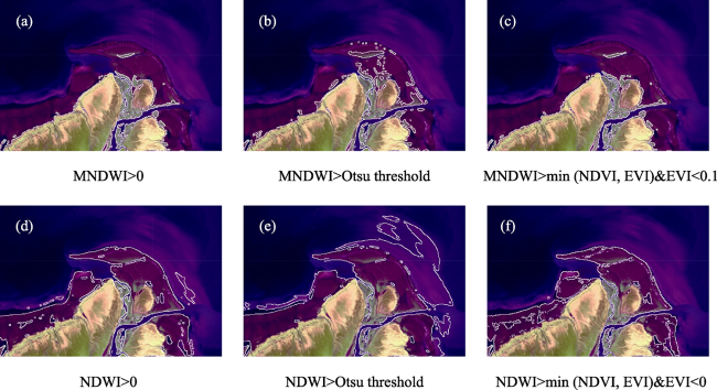
Figure 15 Comparison of various water detection methods commonly used in tidal flat extraction, where the background and white lines are the P60 composite image and surface water boundaries, respectively, corresponding to the decision trees below
Figure 16 shows a detailed comparison of the tidal flat distribution to the Murray Global Intertidal Change Datasets at the Yellow River Mouth and Gaoshaling Port (please refer to the locations in Figure 1). Generally, the area based on Murray’s data was larger than that determined in this study because of the greater extent towards both the ocean at the outside boundary of tidal flats near the Yellow River mouth and the bare lands along the inside boundary of tidal flats in Gaoshaling Port. These differences might stem from the effects of sample points used in the training process of the random forest model (Belgiu and Dragut, 2016) and the lower weight of the vegetation index, which is considered an important indicator that helped improve the accuracy in water body or tidal flat extraction (Zou et al., 2017; Wang et al., 2018).
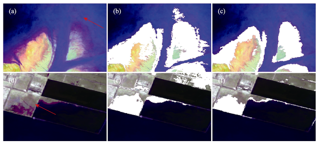
Figure 16 Detailed comparison of the tidal flat distribution to the Murray Global Intertidal Change Datasets at the Yellow River Mouth and Gaoshaling Port. The three columns show the P60 composite images, tidal flat distribution in Murray’s study, and tidal flat distribution in this study from 2014-2016. The white range indicates the extracted tidal flats.
Table 1 and Figure 17 show a regional comparison of the tidal flat area at the city scale to three available tidal flat datasets, including land use and land cover (LULC) data and Murray’s and Zhang’s results (Murray et al., 2019; Zhang et al., 2019). There was a higher consistency with Murray’s study (R2 = 0.97) but a lower consistency with Zhang’s research (R2 = 0.45) or the LULC data (R2 = 0.10) because of the difference in the statistical regions and definitions of tidal flats. Note that there existed a relatively high correlation between Zhang’s and this research in cities near the Liaohe Delta and Yellow River Delta, including Yingkou, Panjin, Jinzhou, Binzhou, Dongying, and Weifang. In other cities, there occurred a smaller area of tidal flats in Zhang’s study because of smaller statistical regions where landward tidal flats disconnected from the shoreline were masked. The poor consistency between the LULC data and other studies was caused by the inclusion of reclaimed regions and exclusion of tidal flats in the open sea in the LULC data for different classification targets (Zhang et al., 2019).
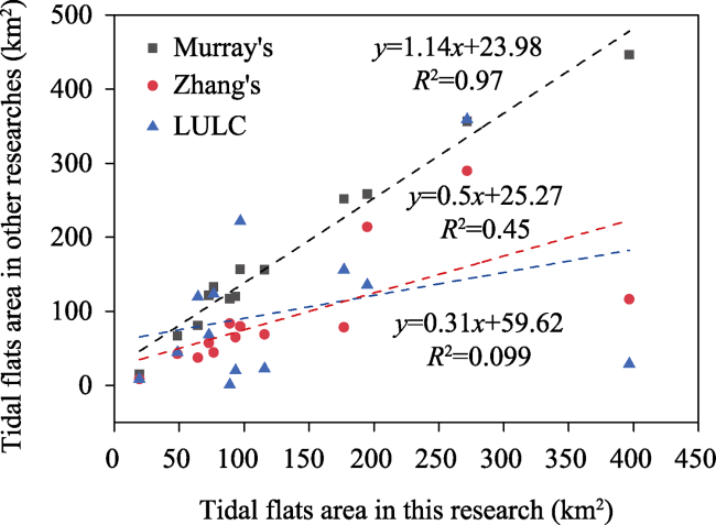
Table 1 Comparison of tidal flat areas to the Murray Global Intertidal Change Datasets, LULC data, and Zhang’s research at the city scale in the Bohai Rim region
Cities around the Bohai Sea Tidal flat area (km2)
Murray’s LULU Zhang’s This study
Dalian 445.88 28.83 116.48 397.00
Yingkou 116.80 0.74 83.55 89.05
Panjin 258.10 135.47 213.71 194.84
Jinzhou 121.60 68.14 57.04 72.81
Huludao 66.93 44.36 42.55 48.77
Qinhuangdao 14.62 8.39 8.27 19.58
Tangshan 251.71 155.84 78.58 176.96
Tianjin 132.97 123.25 44.14 76.73
Cangzhou 156.26 22.59 68.76 115.70
Binzhou 119.77 20.05 64.81 93.39
Dongying 356.09 358.57 289.81 271.95
Weifang 156.51 221.48 79.61 97.08
Yantai 80.81 119.37 37.01 64.32
Figure 17 Linear regression of the tidal flat area at the city scale in the Bohai Rim region for Murray’s study, Zhang’s study, and LULC data in 2015
The uncertainty of tidal flat mapping might originate from Landsat data and algorithms (Wang et al., 2018). Considering the regional difference in the number of effective observations and the availability of fewer observations at very low and very high tide levels, the tidal flat map in this study might not be accurate in every pixel. In this study, all the surface reflectance images of LT05 and LC08 during 1984 to 2019 were selected to reduce the impact of vegetation and tidal dynamics, and the object-based method was selected to reduce the disturbance of noise at the pixel level. As nearly 90% of the locations in the ROI contained more than 300 effective observations in this study, it remains feasible to obtain long-term tidal flat evolution benefits from the large amounts of data covering most tidal ranges and the reliability algorithm to track the movement of the two water boundaries corresponding to Eqs. (5) and (6).

4.2 Driving factors of the evolution of tidal flats around the Bohai Sea

4.2.1 Direct and rapid impact of reclamation

Reclamation exerted a rapid and direct impact on the evolution of tidal flats by changing the land cover and coastal hydrodynamic strength in the short term. Figure 18 shows the distribution of land cover changes during 1984-1986 to 2017-2019. Development existed in the supra-tidal, intertidal, and sub-tidal zones during the expansion of ports, aquafarms, or saltpans, which rapidly and directly altered nearby coastlines. These coastlines also provided a new baseline and formed new buffer zones in the sediment accumulation zone. However, dykes interrupted the balance between the sediment supply and tidal hydrodynamics in coastal regions (Liang et al., 2018) by affecting the flow velocity distribution and blocking coastal sediment transport, and tidal flats in bays near ports could be affected by a reduced sediment storage capability, especially in Bohai Bay. It was reported that the reclamation area in the surrounding three provinces and one municipality around the Bohai Sea reached approximately 7575 km2 from 2000-2015 (Ding et al., 2019), and the proportions of natural shorelines in Liaodong Bay, Bohai Bay, and Laizhou Bay declined to 14.9%, 1.2%, and 19.0%, respectively, in 2018 (Zhang and Niu, 2021), which resulted in reclamation functioning as the most direct and rapid human factor in the evolution of tidal flats in the Bohai Rim region.
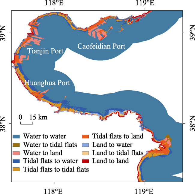
Figure 18 Distribution of land cover changes in the Bohai Rim region from 1984-1986 to 2017-2019

4.2.2 Indirect but continuous impact of the river sediment supply

The river sediment supply, dominated by the sediment load and distance from the estuary, exerted an indirect but continuous impact on the evolution of tidal flats in the delta and even nearby bays in the long term (Bi et al., 2014; Chu et al., 2006). The sediment load of the Yellow River provided the main sediment source in the Bohai Sea area. Among the four large- to medium-sized rivers delivering fresh water and sediments to the Bohai Sea, namely, the Yellow River, Haihe River, Luanhe River, and Liaohe River, the Yellow River exhibited the highest runoff and sediment load, accounting for 77.96% and 96.69%, respectively, of the total amounts (Wang et al., 2014). Figure 19 shows the correlation relationship between the tidal flat area in Dongying and the above two indicators, including the annual runoff and sediment load recorded by the last hydrological station closest to the estuary of the Yellow River, namely, the Lijin Station. The tidal flat area was positively correlated with the annual runoff and sediment load, with R2 = 0.216 and R2 = 0.837, respectively. The reason was that the sediment load constitutes the key source material for the development of tidal flats, while runoff indirectly affects sediment transport towards the estuary.
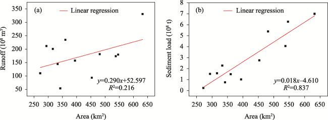
Figure 19 Correlation relationship between the tidal flat area in Dongying and two indicators, including runoff (a) and sediment load (b), at the Lijin Station
The distance from the estuary also affected the sediment supply via the distribution of the abundance, e.g., the growth direction of the Yellow River Delta changed after the artificial branching project in May 1996 to promote land development near the northern oil fields. Figure 20 shows the evolution of the outer boundaries of the tidal flats near the Yellow River Delta during 1984 to 2019 and the maximum distance from various intersecting points to the origin point. The distances along the two directions exhibited opposite trends before and after estuary position change, and the rate of change was reduced. The main reason was that the change in the estuary position directly affected the sediment supply in nearby regions. The regions near the new estuary gained a more abundant sediment supply to promote tidal flat growth. The regions near the abandoned estuary lost a part of the sediment supply, and it was difficult to maintain the existing balance between erosion and deposition, where these tidal flats were continuously eroded under hydrodynamic action. Under the combined action of hydrodynamics and the sediment supply, sediment accumulation gradually tended to establish a new balance. In addition, the growth rate of the Yellow River Delta near the new estuary declined. The long-term lower levels of the runoff and sediment load of the Yellow River (Song et al., 2020) could cause a potentially lower sediment supply and even erosion problems in tidal flats and limit growth in the Yellow River Delta.
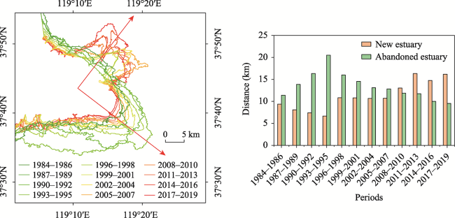
Figure 20 Evolution of the outer boundaries of the tidal flats near the Yellow River Delta during 1984 to 2019 and the maximum distance between the coastlines and parallel coordinate axes, where the x- and y-axes illustrate the direction of the new and abandoned estuaries, respectively

4.2.3 High potential impact of relative sea-level rise

The relative sea-level rise caused by both sea-level rise and ground subsidence is often a slow but persistent, accumulative, and irreversible process (Wei et al., 2015; Zhang et al., 2015). Affected by local runoff and precipitation, there usually existed a high sea level in August, and the affected region was much larger. Figure 21 shows the monthly average sea level of the Bohai Sea in August during 1980-2019 and its negative correlation with the tidal flat area in the Bohai Rim region. The average value from 1975 to 1986 is commonly used when calculating the long-term average value. There occurred a severe fluctuation and upward trend in the sea level of the Bohai Sea in August and an obvious negative correlation with the tidal flat area in the Bohai Rim region. According to the China Sea Level Bulletin in 2019, the sea level of the Bohai Sea will continue to rise by 55-180 mm over the next 30 years, which will enhance the effect of storm surges or tidal flat erosion and increase the difficulty of coastal remediation. Land subsidence might lead to a further increase in the relative sea level, weaken the function of nearshore protection facilities or strengthen hydrodynamic effects, and eventually increase the risk of coastal erosion and submergence, especially in alluvial plains. The contribution of subsidence to relative sea-level change greatly varies across regions. It was reported that there occurred relatively notable land subsidence in Tianjin and Shanghai in China according to the Sea Level Bulletin of 2020, e.g., 17 mm in the Tianjin Binhai New Area. Subsidence was usually caused by excessive groundwater withdrawal, neotectonic movement, sediment consolidation, compaction, and oil extraction (Xue et al., 2005; Zhang et al., 2015). Therefore, the relative sea-level rise might exert a high potential negative impact on the protection of tidal flats.
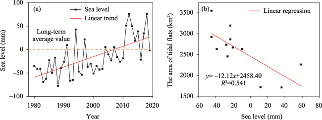
Figure 21 Monthly average sea level in August of the Bohai Sea during 1980-2019 and its correlation analysis with the tidal flat area in the Bohai Rim region

5 Conclusions

In this paper, a decision tree algorithm for tidal flat extraction was developed, and spatiotemporal variations in tidal flats and coastlines in the Bohai Rim region during 1984-2019 were analysed based on 9539 Landsat images over twelve periods and the GEE cloud platform. The following conclusions could be drawn:
(1) The combination of two decision trees for surface water detection, including Eq. (5) proposed by Wang et al. and Eq. (6) proposed in this study, could allow potential applications in tracking boundaries between land, tidal flats, and permanent water regions with fewer calculations and a higher automation level. The tidal flat distribution obtained according to the tidal flat extraction process in Section 2.3 exhibited a high accuracy and consistency with Murray Global Intertidal Change Datasets data.
(2) The area of tidal flats in the Bohai Rim region fluctuated downwards from 3551.22 km2 to 1712.36 km2 during 1984-2019. During 2017-2019, 51.31% of the tidal flats was mainly distributed in six cities near the Yellow River Delta and Liaohe River Delta, including Weifang, Dongying, Cangzhou, Jinzhou, Panjin, and Yingkou. There occurred a drastic spatial transition during 1984-2019, and tidal flats with a low stability were mainly distributed in deltas and reclamation regions. The length of the coastline in the Bohai Rim region increased by 17.88%, and the coastline migrated towards the ocean, especially after 2000. The average EPR during 2000-2018 was 120.36 m/a, approximately 5 times the rate during 1985-2000 near the Bohai Sea.
(3) Reclamation exerted a rapid and direct impact on the evolution of tidal flats by changing the land cover and coastal hydrodynamic strength in the short term. A long-term reduced sediment supply exerted a continuous negative impact on tidal flat growth. The relative sea-level rise potentially deteriorated the function of nearshore protection facilities and strengthened hydrodynamic effects.
In follow-up research, the application of this tidal flat extraction process will be expanded to high-resolution and high-frequency remote sensing data, e.g., Sentinel images, considering the image series length meets the requirements. The impact of hydrodynamics and suspended sediment transport on tidal flat evolution will also be considered during the exploration of the dynamic process of tidal flat evolution on a smaller spatial or temporal scale. The extraction process and tidal flat maps herein could provide references for soil and water conservation near the coastline.
[1]
Achanta R, Süsstrunk S, 2017. Superpixels and polygons using simple non-iterative clustering. 2017 IEEE Conference on Computer Vision and Pattern Recognition (CVPR): 4895-4904.

[2]
Belgiu M, Dragut L, 2016. Random forest in remote sensing: A review of applications and future directions. Isprs Journal of Photogrammetry and Remote Sensing, 114: 24-31.

DOI

[3]
Bi N H, Wang H J, Yang Z H, 2014. Recent changes in the erosion-accretion patterns of the active Huanghe (Yellow River) Delta lobe caused by human activities. Continental Shelf Research, 90: 70-78.

DOI

[4]
Blum M D, Roberts H H, 2009. Drowning of the Mississippi Delta due to insufficient sediment supply and global sea-level rise. Nature Geoscience, 2(7): 488-491.

DOI

[5]
Boak E H, Turner I L, 2005. Shoreline definition and detection: A review. Journal of Coastal Research, 21(4): 688-703.

[6]
Chen G, Ye Z, Jin R et al., 2021. Spatial-temporal distribution of salt marshes in intertidal zone of China during 1985-2019. Preprints 2021, 2021040146.

[7]
Chen J, Ban Y, Li S, 2014. China: Open access to Earth land-cover map. Nature, 514(7523): 434-434.

[8]
Chen Y, Dong J, Xiao X et al., 2016. Land claim and loss of tidal flats in the Yangtze Estuary. Scientific Reports, 6(1): 24018.

DOI

[9]
Chu Z X, Sun X G, Zhai S K et al., 2006. Changing pattern of accretion/erosion of the modem Yellow River (Huanghe) subaerial delta, China: Based on remote sensing images. Marine Geology, 227(1/2): 13-30.

DOI

[10]
Dada O A, Li G X, Qiao L L et al., 2016. Seasonal shoreline behaviours along the arcuate Niger Delta coast: Complex interaction between fluvial and marine processes. Continental Shelf Research, 122: 51-67.

DOI

[11]
Ding X, Shan X, Chen Y et al., 2019. Dynamics of shoreline and land reclamation from 1985 to 2015 in the Bohai Sea, China. Journal of Geographical Sciences, 29(12): 2031-2046.

DOI

[12]
Donchyts G, Schellekens J, Winsemius H et al., 2016. A 30 m resolution surface water mask including estimation of positional and thematic differences using Landsat 8, SRTM and OpenStreetMap: A case study in the Murray-Darling Basin, Australia. Remote Sensing, 8(5): 386-407.

DOI

[13]
Friedl M A, McIver D K, Hodges J C F et al., 2002. Global land cover mapping from MODIS: Algorithms and early results. Remote Sensing of Environment, 83(1/2): 287-302.

DOI

[14]
Fu X-M, Tang H-Y, Liu Y et al., 2021. Resource status and protection strategies of mangroves in China. Journal of Coastal Conservation, 25(4): 42.

DOI

[15]
Ge Z M, Cao H B, Cui L F et al., 2015. Future vegetation patterns and primary production in the coastal wetlands of East China under sea level rise, sediment reduction, and saltwater intrusion. Journal of Geophysical Research Biogeosciences, 120: 1923-1940.

DOI

[16]
Ghorbanian A, Kakooei M, Amani M et al., 2020. Improved land cover map of Iran using Sentinel imagery within Google Earth Engine and a novel automatic workflow for land cover classification using migrated training samples. Isprs Journal of Photogrammetry and Remote Sensing, 167: 276-288.

DOI

[17]
Ghosh S, Mishra D R, Gitelson A A, 2016. Long-term monitoring of biophysical characteristics of tidal wetlands in the northern Gulf of Mexico: A methodological approach using MODIS. Remote Sensing of Environment, 173: 39-58.

DOI

[18]
Han Q, Niu Z, Wu M et al., 2018. Remote-sensing monitoring and analysis of China intertidal zone changes based on tidal correction. Chinese Science Bulletin, 64(4): 456-473.

[19]
Hansen M C, Potapov P V, Moore R et al., 2013. High-resolution global maps of 21st-century forest cover change. Science, 342(6160): 850-853.

DOI PMID

[20]
He T, Xiao W, Zhao Y L et al., 2020. Identification of waterlogging in eastern China induced by mining subsidence: A case study of Google Earth Engine time-series analysis applied to the Huainan coal field. Remote Sensing of Environment, 242: 111742.

DOI

[21]
Huang H, Chen W, Zhang Y et al., 2021. Analysis of ecological quality in Lhasa Metropolitan Area during 1990-2017 based on remote sensing and Google Earth Engine platform. Journal of Geographical Sciences, 31(2): 265-280.

DOI

[22]
Huete A, Didan K, Miura T et al., 2002. Overview of the radiometric and biophysical performance of the MODIS vegetation indices. Remote Sensing of Environment, 83(1/2): 195-213.

DOI

[23]
Jia M, Wang Z, Mao D et al., 2021. Rapid, robust, and automated mapping of tidal flats in China using time series Sentinel-2 images and Google Earth Engine. Remote Sensing of Environment, 255: 112285.

DOI

[24]
Kumar L, Mutanga O, 2018. Google Earth Engine applications since inception: Usage, trends, and potential. Remote Sensing, 10(10): 1509.

DOI

[25]
Liang H, Kuang C, Olabarrieta M et al., 2018. Morphodynamic responses of Caofeidian channel-shoal system to sequential large-scale land reclamation. Continental Shelf Research, 165: 12-25.

DOI

[26]
Liu X, Gao Z, Ning J et al., 2016. An improved method for mapping tidal flats based on remote sensing waterlines: A case study in the Bohai Rim, China. IEEE Journal of Selected Topics in Applied Earth Observations & Remote Sensing, 9(11): 5123-5129.

[27]
Luo W, Yuan L, Yu Z et al., 2011. Regional sea level change in Northwest Pacific: Process, characteristic and prediction. Journal of Geographical Sciences, 21(3): 387-400.

DOI

[28]
Masek J G, Wulder M A, Markham B et al., 2020. Landsat 9: Empowering open science and applications through continuity. Remote Sensing of Environment, 248: 111968.

DOI

[29]
Mason D C, Scott T R, Dance S L, 2010. Remote sensing of intertidal morphological change in Morecambe Bay, U.K., between 1991 and 2007. Estuarine Coastal & Shelf Science, 87(3): 487-496.

[30]
McFeeters S K, 1996. The use of the normalized difference water index (NDWI) in the delineation of open water features. International Journal of Remote Sensing, 17(7): 1425-1432.

DOI

[31]
Murray N J, Phinn S R, Clemens R S et al., 2012. Continental scale mapping of tidal flats across East Asia using the Landsat Archive. Remote Sensing, 4(11): 3417-3426.

DOI

[32]
Murray N J, Phinn S R, DeWitt M et al., 2019. The global distribution and trajectory of tidal flats. Nature, 565(7738): 222-225.

DOI

[33]
Passeri D L, Hagen S C, Medeiros S C et al., 2015. The dynamic effects of sea level rise on low-gradient coastal landscapes: A review. Earth’s Future, 3(6): 159-181.

DOI

[34]
Polte P, Schanz A, Asmus H, 2005. The contribution of seagrass beds (Zostera noltii) to the function of tidal flats as a juvenile habitat for dominant, mobile epibenthos in the Wadden Sea. Marine Biology, 147(3): 813-822.

DOI

[35]
Qiu S, Zhu Z, He B B, 2019. Fmask 4.0: Improved cloud and cloud shadow detection in Landsats 4-8 and Sentinel-2 imagery. Remote Sensing of Environment, 231: 111205.

DOI

[36]
Ren H R, Li G S, Cui L L et al., 2015. Multi-scale variability of water discharge and sediment load into the Bohai Sea from 1950 to 2011. Journal of Geographical Sciences, 25(1): 85-100.

DOI

[37]
Robert J, Hoeksema, 2007. Three stages in the history of land reclamation in the Netherlands. Irrigation and Drainage, 56(Suppl.1): S113-S126.

DOI

[38]
Sagar S, Roberts D, Bala B et al., 2017. Extracting the intertidal extent and topography of the Australian coastline from a 28 year time series of Landsat observations. Remote Sensing of Environment, 195: 153-169.

DOI

[39]
Shi W J, Liu Y T, Shi X L, 2017. Development of quantitative methods for detecting climate contributions to boundary shifts in farming-pastoral ecotone of northern China. Journal of Geographical Sciences, 27(9): 1059-1071.

DOI

[40]
Song X, Zhong D, Wang G, 2020. Simulation on the stochastic evolution of hydraulic geometry relationships with the stochastic changing bankfull discharges in the Lower Yellow River. Journal of Geographical Sciences, 30(5): 843-864.

DOI

[41]
Stehman S V, 1997. Selecting and interpreting measures of thematic classification accuracy. Remote Sensing of Environment, 62(1): 77-89.

DOI

[42]
Temmerman S, Meire P, Bouma T J et al., 2013. Ecosystem-based coastal defence in the face of global change. Nature, 504(7478): 79-83.

DOI

[43]
Tucker C J, 1979. Red and photographic infrared linear combinations for monitoring vegetation. Remote Sensing of Environment, 8(2): 127-150.

DOI

[44]
Wang H, Wang A, Bi N et al., 2014. Seasonal distribution of suspended sediment in the Bohai Sea, China. Continental Shelf Research, 90: 17-32.

DOI

[45]
Wang X, Xiao X, Zou Z et al., 2018. Tracking annual changes of coastal tidal flats in China during 1986-2016 through analyses of Landsat images with Google Earth Engine. Remote Sensing of Environment, 238: 110987.

DOI

[46]
Wei W, Tang Z, Dai Z et al., 2015. Variations in tidal flats of the Changjiang (Yangtze) estuary during 1950s-2010s: Future crisis and policy implication. Ocean & Coastal Management, 108: 89-96.

[47]
Xu H, 2006. Modification of normalised difference water index (NDWI) to enhance open water features in remotely sensed imagery. International Journal of Remote Sensing, 27(14): 3025-3033.

DOI

[48]
Xue Y Q, Zhang Y, Ye S J et al., 2005. Land subsidence in China. Environmental Geology, 48(6): 713-720.

DOI

[49]
Yan H, Dai Z, Li J et al., 2011. Distributions of sediments of the tidal flats in response to dynamic actions, Yangtze (Changjiang) Estuary. Journal of Geographical Sciences, 21(4): 719-732.

DOI

[50]
Yu T, Douglas S, Chen H et al., 2018. Mapping vegetation and land use types in Fanjingshan National Nature Reserve using Google Earth Engine. Remote Sensing, 10(6): 927.

DOI

[51]
Zhang J, Huang H, Bi H, 2015. Land subsidence in the modern Yellow River Delta based on InSAR time series analysis. Natural Hazards, 75(3): 2385-2397.

DOI

[52]
Zhang K Y, Dong X Y, Liu Z G et al., 2019. Mapping tidal flats with Landsat 8 images and Google Earth Engine: A case study of the China’s eastern coastal zone circa 2015. Remote Sensing, 11(8): 924-943.

DOI

[53]
Zhang T, Niu X, 2021. Analysis on the utilization and carrying capacity of coastal tidal flat in bays around the Bohai Sea. Ocean & Coastal Management, 203: 105449.

[54]
Zou Z, Dong J, Menarguez M A et al., 2017. Continued decrease of open surface water body area in Oklahoma during 1984-2015. Science of The Total Environment, 595(Oct.1): 451-460.

DOI

[55]
Zou Z, Xiao X, Dong J et al., 2018. Divergent trends of open-surface water body area in the contiguous United States from 1984 to 2016. PNAS, 115(15): 3810-3815.

DOI PMID

Outlines

/