Research Articles

Drivers of water pollutant discharge in urban agglomerations and their scale effects: Empirical analysis of 305 counties in the Yangtze River Delta

  • ZHOU Kan , 1, 2 ,
  • YIN Yue 1, 2 ,
  • CHEN Yufan 1, 2
Expand
  • 1. Key Laboratory of Regional Sustainable Development Modeling, Institute of Geographic Sciences and Natural Resources Research, CAS, Beijing 100101, China
  • 2. University of Chinese Academy of Sciences, Beijing 100049, China

Zhou Kan (1986-), PhD and Associate Professor, specialized in resources and environmental carrying capacity and regional sustainable development. E-mail:

Received date: 2022-07-16

  Accepted date: 2022-09-17

  Online published: 2023-01-16

Supported by

National Natural Science Foundation of China(41971164)

Strategic Priority Research Program of the Chinese Academy of Sciences(XDA23020101)

Abstract

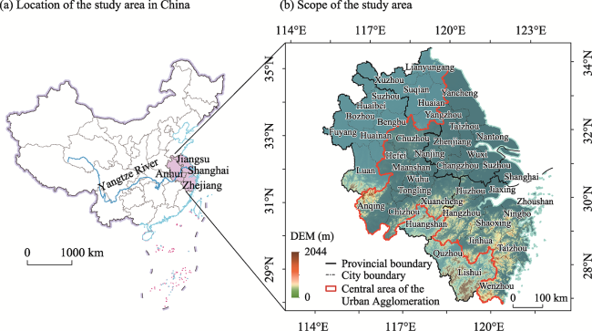
Revealing the drivers and scale effects of water pollutant discharges is an important issue in the study of the environmental consequences during urban agglomeration evolution. It is also a prerequisite for realizing collaborative water pollutant reduction and environmental governance in urban agglomerations. This paper takes 305 counties in the Yangtze River Delta (YRD) as an example and selects chemical oxygen demand (COD) and ammonia nitrogen (NH3-N) as two distinctive pollutant indicators, using the Spatial Lag Model (SLM) and Spatial Error Model (SEM) to estimate the drivers of water pollutant discharges in 2011 and 2016. Then the Multiscale Geographically Weighted Regression (MGWR) model is constructed to diagnose the scale effect and spatial heterogeneity of the drivers. The findings show that the size of population, the level of urbanization, and the economic development level show global-level increase impacts on water pollutant discharges, while the level of industrialization, social fixed assets investment, foreign direct investment, and local fiscal decentralization are local-level impacts. The spatial heterogeneity of local drivers presents the following characteristics: Social fixed assets investment has a strong promoting effect on both COD and NH3-N discharges in the Hangzhou-Jiaxing-Huzhou region and the coastal area of the YRD; industrialization has a promoting effect on COD discharges in the Taihu Lake basin and Zhejiang province; foreign direct investment has a local inhibitory effect on NH3-N discharge, and the pollution halo effect is more prominent in the marginal areas of the YRD such as northern Jiangsu, northern Anhui, and southern Zhejiang; local fiscal decentralization has a noticeable inhibitory effect on COD discharge in the central areas of the YRD, reflecting the positive impacts on improved local environmental awareness and stronger constraints of multilevel environmental regulations in the urban agglomeration. Therefore, it is recommended to guide greener development to reduce the water pollutant discharge; to embed an environmental push-back mechanism in the fields of industrial production, capital investment, and financial income and expenditure; and to establish a high-quality development pattern of urban agglomerations systematically compatible with the carrying capacity of the water environment.

Cite this article

ZHOU Kan , YIN Yue , CHEN Yufan . Drivers of water pollutant discharge in urban agglomerations and their scale effects: Empirical analysis of 305 counties in the Yangtze River Delta[J]. Journal of Geographical Sciences, 2023 , 33(1) : 195 -214 . DOI: 10.1007/s11442-022-2066-6

1 Introduction

As an integrated urban community, the development of urban agglomerations is always accompanied by the gathering of populations and economic activities, and expanding of impervious surfaces (Zhu et al., 2011; Fang, 2014; Fan et al., 2021). Meanwhile, the growing urban agglomeration inevitably increased anthropogenic pollutants to the regional ecosystem, and produced some negative externalities such as environmental structural disorders, functional degradation, and even system collapse. For instance, previous studies showed that urban agglomerations have triggered a surge in the intensity and scale of various pollutant discharges (Gong et al., 2012; Al-Mulali et al., 2015; Lu et al., 2019; Zhou et al., 2020). In this regard, promoting collaborative water environment management and regulation in urban agglomerations across cities and administrative boundaries which has received wide attention from academics and policymakers (Yao et al., 2016; Fang et al., 2018).
Many researchers have focused on the relationships among socioeconomic activities, atmospheric pollution, and environmental effects in urban agglomerations’ evolution, mainly using air quality data, satellite remote sensing information, and other means to analyze atmospheric environmental pollution caused by various anthropogenic source discharges during the spatial expansion and structural evolution of urban agglomerations (Ghosh et al., 2012; Sun et al., 2016; Singh et al., 2017). In the current phase of the stalemate between overall improvement and local environmental quality deterioration, many studies have conducted in-depth research on pollution mechanisms, cross-regional mobility, and carbon discharge rights from different perspectives. These studies revealed the spatial spillover effects of urbanization and industrialization on air pollution discharges and proposed the importance of joint regional air pollution management (Chen et al., 2018; Li et al., 2018; Wang, 2020).
In the field of water pollution, more studies have been conducted on various lakes, sea areas, and inland water systems in urban agglomerations as receptors of water pollution discharge, and experimental data are obtained through sampling and testing. These studies focused on water quality, water environment, and water ecology changes and responses caused by the development of urban agglomerations (Chang, 2005; Tasdighi et al., 2017; Alimi et al., 2018). In addition, some researchers studied the socioeconomic drivers such as economic growth, population and urbanization, environmental regulation, and financial investment to explore the water environment effects and drivers of urban agglomeration’s evolution. Among these, the relationship between economic growth and anthropogenic pollutant discharges is portrayed from the perspective of economic growth drivers using the environmental Kuznets curve (EKC) (Grossman et al., 1995). Then fitting characteristics between pollutant indicators such as industrial wastewater, industrial waste gas, industrial solid waste, and economic growth are investigated by panel data to test the EKC hypothesis at the scale of urban agglomerations or larger regions (Akca et al., 2012; Cheng, 2012; Guo et al., 2017).
Through studies on the social drivers of population, the effects of population size and urbanization on anthropogenic pollutant discharges have been examined; the Stochastic Impacts by Regression on Population, Affluence and Technology (STIRPAT) model found a correlation between the two factors, with population size growth and increased urbanization levels significantly increasing pollutant discharges (Cole et al., 2004; Wang et al., 2018; Liang et al., 2019). Other studies have focused on the effects of environmental regulations, financial inputs, and other drivers, revealing that environmental regulations are important tools to reduce pollution discharges and inhibit pollution transfer, but the effectiveness of the same environmental regulation varies by pollutant (Böcher, 2012; Morley, 2012; Ahmad et al., 2020; Ulucak et al., 2020). The impact of foreign investment on environmental pollution has been viewed in various ways. Some researchers believe that the inflow of foreign direct investment (FDI) aggravates environmental pollution in the host country and have identified the pollution paradise effect—especially in the early industrialization period—when developing countries took on a large number of pollution-intensive industries due to the low intensity of environmental regulations (Cole et al., 2011; Liao et al., 2015; Hamid et al., 2021). In contrast, some studies have shown that FDI also has a pollution halo effect on environmental pollution in the host country, because the technological progress and spillover effects brought by FDI will improve local abatement processes and pollution control efficiency (He, 2006; Sheng et al., 2012; Zhou et al., 2019). Thus, many longitudinal studies at national, provincial, and municipal scales and horizontal studies on the formation, causes, and management of water pollution have found that the development of urban agglomerations significantly increases the regional water resources and water environment load.
In the future—under the realistic demand for pollution reduction and high-quality human living environments in urban agglomerations—revealing the drivers and spatial environmental effects of water pollutant discharges will become a hot topic for urban agglomeration formation and development. This is an important basis for realizing high-quality development and positive interactions between socioeconomic aspects and the ecological environment of urban agglomerations. However, existing studies fail to explain well the driving intensity and divergent characteristics of water pollution discharge at different spatial scales. It is difficult to quantify the influence mechanism of water pollutant discharge during the development of urban agglomerations at the local level, and it is urgent to close the gap of insufficient research on the relationship between socioeconomic drivers and water pollutant discharge. Given this background, this paper selects the Yangtze River Delta urban agglomerations as a typical region and attempts to study the issue through a combination of global and local regression modeling. Based on the overall estimation of county-scale water pollutant discharge drivers, the Multiscale Geographically Weighted Regression (MGWR) model is applied to diagnose the scale effects and spatial heterogeneity of the drivers to lay a good foundation for the design of environmental quality development pathways and water pollution reduction policies in urban agglomerations.

2 Data and methods

2.1 Study area and data sources

The Yangtze River Delta urban agglomeration covers the entirety of Shanghai, Jiangsu, Zhejiang, and Anhui provinces, with a total land area of 358,000 km2. It includes the central area of the urban agglomeration consisting of the Shanghai, Nanjing, Hangzhou, Hefei, Suzhou-Wuxi-Changzhou, and Ningbo metropolitan areas (Figure 1), as well as the fringe areas radiating from the coastal development belt and the riverine development belt. The YRD is one of the strongest economic regions in China, leading the economic development of the Yangtze River Economic Belt and even the whole country. The resident population totals 221 million, accounting for 16.06% of the total population of China, with a gross domestic product (GDP) of RMB 16.01 trillion, accounting for 23.36% of the national GDP (SCPRC, 2019). However, rapid urban expansion and resource consumption have led to high-intensity water pollutant discharges in the YRD. The region occupies 4% of the national land area and carries 21% of the national wastewater discharges. At the end of 2016, the chemical oxygen demand (COD) and ammonia nitrogen (NH3-N) discharges in the YRD were 185.17×10⁷ kg and 27.05×10⁷ kg, respectively accounting for 17.69% and 19.08% of the national total (Table 1). High discharges have led to prominent water pollution problems and serious regional water ecological imbalance in the YRD. Measurements of county water quality show that the proportion of counties exceeding the annual average concentrations of COD and NH3-N are 18.93% and 16.43%, while those exceeding the critical limit are 35.71% and 25.36%. This indicates that water pollution in local areas is threatening the safety of drinking water.
Figure 1 Location and scope of the study area (Yangtze River Delta)
Table 1 Regional comparison of water pollutant discharge in the Yangtze River Delta in 2016
Region Chemical oxygen demand Ammonium-nitrogen
Total regional discharges
(×104 t)
Share of total discharges
(%)
County discharges intensity
(t)
Total regional discharges
(×104 t)
Share of total discharges
(%)
County discharges intensity
(t)
Shanghai 14.75 1.41 9219.18 3.84 2.71 2397.84
Jiangsu 74.65 7.13 6785.98 10.28 7.25 934.24
Zhejiang 46.14 4.41 4394.73 7.30 5.15 695.30
Anhui 49.63 4.74 4205.99 5.63 3.97 477.51
YRD 185.17 17.69 6071.21 27.05 19.08 886.84
In this work, a water pollutant discharge and socioeconomic database was established for 305 county-level administrative districts in the YRD, namely counties, districts, and county-level cities. The administrative boundary data were obtained from the website of the National Geomatics Center of China (http://www.ngcc.cn/ngcc/). County land use status data were collected from natural resources authorities. Pollutant discharge and socioeconomic data were mainly from the 2011-2016 China County Statistical Yearbook, Shanghai Statistical Yearbook, Jiangsu Statistical Yearbook, Zhejiang Provincial Statistical Yearbook, Anhui Provincial Statistical Yearbook, and the relevant county departments of ecology and environment. For the 33 county units with incomplete or missing data, city or county statistical yearbooks and bulletins were obtained to make up for the lack.

2.2 Methods and variables

2.2.1 Estimation model of drivers

According to the spatial mobility characteristics of water pollution and theoretical analysis, the process of water pollutant discharge from urban agglomerations has spatial spillover effects. To incorporate spatial correlation and spatial heterogeneity into the driver analysis, the spatial lag model (SLM) and spatial error model (SEM) were used for spatial autocorrelation regression analysis (Anselin, 1988; Jiang et al., 2009). The SLM model uses a spatial lag term to assess spatial interactions and analyzes the spatial spillover effects of water pollutant discharges from county units to neighboring counties. Its model formulation is given by Equation (1):
Y = ρWy + βX + ε
where Y is the explained variable, and X is the matrix of exogenous explanatory variables. ρ is the spatial regression coefficient to reflect the degree of spatial dependence, and β is the coefficient to be estimated. Wy is the spatially lagged dependent variable and ε is the random error vector.
The SEM model, which uses a spatial error term to measure the influence on the county of the error shock of the explanatory variables in neighboring county units, is expressed as Equation (2):
Y = βX + ε, ε = λWε + μ
where λ is the spatial error coefficient to reflect the degree of spatial dependence present in the error term, Wε is the spatial weight matrix of the error term, ε is the random perturbation term, and μ is the random error vector.

2.2.2 Diagnostic model of scale effect

Unlike the traditional geographically weighted regression (GWR) model, which assumes that all drivers act on the dependent variable at the same spatial scale, the MGWR allows the response to variations in the relationship between variables and explanatory variables at spatial and different scales (Fotheringham et al., 2017; Yu et al., 2020). Thus, MGWR can better explore the scale effects and spatial differentiation of the drivers. The basic model is given as follows:
${{y}_{i}}=\underset{j=1}{\overset{k}{\mathop \sum }}\,{{\beta }_{bij}}({{u}_{i}},{{v}_{i}}){{x}_{ij}}+{{\varepsilon }_{i}}$
where βbij denotes the regression coefficient of the local variable and bij denotes the bandwidth used for the regression coefficient of variable j. (ui,vi) represents the geographical coordinates of county i, xij is the observation of variable j at county i, and εi is a random disturbance term. Each regression coefficient β of the MGWR is obtained based on local regression, and the bandwidth possesses heterogeneity. Compared with the GWR model, the MGWR model reduces covariance and bias in the parameter estimation by accurately depicting the spatial heterogeneity. In addition, MGWR uses the most commonly used quadratic kernel function and the corrected Akaike Information Criterion (AICc) in GWR (Wolf et al., 2018; Oshan et al., 2019).

2.2.3 Variables and their descriptions

The selected variables include water pollutant discharges and socioeconomic drivers; data from 305 county units in the YRD from 2011 to 2016 are aggregated. Indicators were selected as follows:
Explained variables: COD and NH3-N variables. Environmental authorities use COD and NH3-N as the main control pollutants in water environmental protection planning and implementation management through total control targets. Conversely, the two water pollutants in the study area bear an important share of discharge reduction targets within the framework of China and Yangtze River Basin water pollutant regulations, and the discharge control is more stringent than control of other pollutants.
Explanatory variables: Based on the established theoretical framework and empirical research, the socioeconomic development variables that may affect water pollutant discharges were selected as explanatory variables (Table 2). POP represents the year-end resident population, which characterizes the size of the resident population in the county. UR represents the urbanization rate, which characterizes the level of urbanization in the county. The growth of population size and urbanization level generally has a promoting effect and increases the discharge of various pollutants from domestic sources (Cole et al., 2004; Wang et al., 2018; Liang et al., 2019). PGDP represents per capita GDP, which characterizes the level of county economic development. According to the general rule of the EKC, as the level of economic development increases, per capita GDP and pollutant discharges show an inverted U-shaped relationship of promoting and then inhibitory effects (Grossman et al., 1995; Akca et al., 2012; Cheng, 2012; Guo et al., 2017). IS represents the ratio of secondary industry value added to GDP, which characterizes the industrial structure and industrialization level of the county. Industrialization, especially the expansion of pollution-intensive manufacturing, usually causes an increase in pollutant discharges from industrial sources (Akca et al., 2012; Cheng, 2012; Guo et al., 2017). FDI is used to characterize the degree of market openness in counties, where foreign investment may have both a pollution paradise effect that increases pollution in the investment site and a pollution halo effect that suppresses pollution discharges due to the introduction of environmental disposal technologies (He, 2006; Cole et al., 2011; Sheng et al., 2012; Liao et al., 2015; Jin et al., 2016; Zhou et al., 2019). FAI represents the amount of social fixed asset investment, characterizing the scale of capital investment and asset reproduction capacity in the county; capital expansion usually leads to a significant increase in water pollutant discharges (Wen et al., 2015; Luo et al., 2019). FD represents the ratio of local fiscal revenues to local fiscal expenditures and characterizes the local fiscal decentralization in counties. With the shift in environmental awareness, local governments will have the ability and willingness to change previous lax environmental regulations when they have more fiscal autonomy, which leads to a shift from promoting to inhibiting effects in pollutant discharges (Böcher, 2012; Morle, 2012; Yu et al., 2015; Ulucak et al., 2020).
Table 2 Descriptive statistics of the main explanatory variables in 2016
Variable Description Code Mean Standard deviation Maximum Minimum
Size of resident population (×104 person) POP 68.37 41.54 295.77 7.62
Urbanization level (%) UR 68.20 21.29 100.00 24.18
Economic development level (yuan/person) PGDP 85,966.22 69,992.29 422,517.88 7544.21
Industrialization level (%) IS 43.08 13.66 80.10 2.84
Foreign direct investment (×104 USD) FDI 258,452.59 416,389.60 1,851,378.00 6109.00
Social fixed asset investment (×108 yuan) FAI 335.12 230.41 1825.74 8.98
Degree of local fiscal decentralization (%) FD 74.09 39.27 244.10 13.22

3 Results

3.1 Spatiotemporal pattern analysis

During 2011-2016, water pollutant discharges in the YRD significantly decreased, with total COD and NH3-N discharges decreasing by 41.36% and 35.54%, respectively, at rates of -10.13% and -8.41% per year, respectively. The average COD discharge intensity in the YRD counties dropped from 10328.42 t in 2011 to 6056.58 t in 2016, and NH3-N discharge intensity dropped from 1373.67 t to 885.50 t. The distribution of water pollutant discharge intensity in each county is shown in Figure 2. The overall pattern of high-intensity, contiguous water pollutant discharges in the YRD has improved significantly. In particular, the number of counties with high discharge intensity in the central area of the urban agglomeration has sharply declined. The number of counties with COD discharge intensity greater than 20,000 t in the central area reduced from 22 in 2011 to 4 in 2016, and those with NH3-N discharge intensity greater than 2000 t in the central area reduced from 50 to 11. By 2016, the high discharge areas in the YRD were mainly distributed in the Taihu Lake basin, the eastern coast, the northern Anhui region, and the metropolitan areas of Shanghai, Nanjing, and Suzhou-Wuxi-Changzhou, and showed a core-edge pattern of decreasing discharge intensity from the central urban areas to the suburban counties.
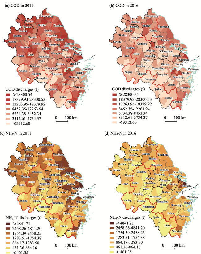
Figure 2 Classification of water pollutant discharge intensity at the county level in the Yangtze River Delta (a. chemical oxygen demand (COD) in 2011; b. COD in 2016; c. ammonium-nitrogen (NH3-N) in 2011; d. NH3-N in 2016)
The hot spot analysis using the Getis-Ord Gi* index further indicated that the water pollutant discharge pattern in the YRD counties showed a relatively stable distribution of high and low values (Figures 3 and 4). During 2011-2016, the number of counties in hotspots and sub-hotspots of COD discharge intensity was maintained at more than 130 (Figure 3), stably distributed in Shanghai metropolitan area; Nanjing metropolitan area; Hefei metropolitanarea; Yancheng, Lianyungang, Xuzhou, Suqian, Huaibei, Huainan, and other northern Jiangsu and northern Anhui cities; and also scattered in Shaoxing, Wenzhou, Taizhou, and other cities. The Gi* index value of NH3-N discharge intensity decreased from the coastal development belt counties to inland counties, where the hot spot areas were concentrated in Shanghai and surrounding counties. Therefore, despite the significant trend of water pollutant reduction in the YRD, the clustering pattern of high water pollution discharge counties remained stable, especially in the coastal and riverine areas in the central area of the YRD; northern Jiangsu Province was spatially locked (Figure 4).
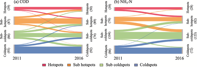
Figure 3 Changes in the distribution of hotspots and coldspots in the Yangtze River Delta from 2011 to 2016
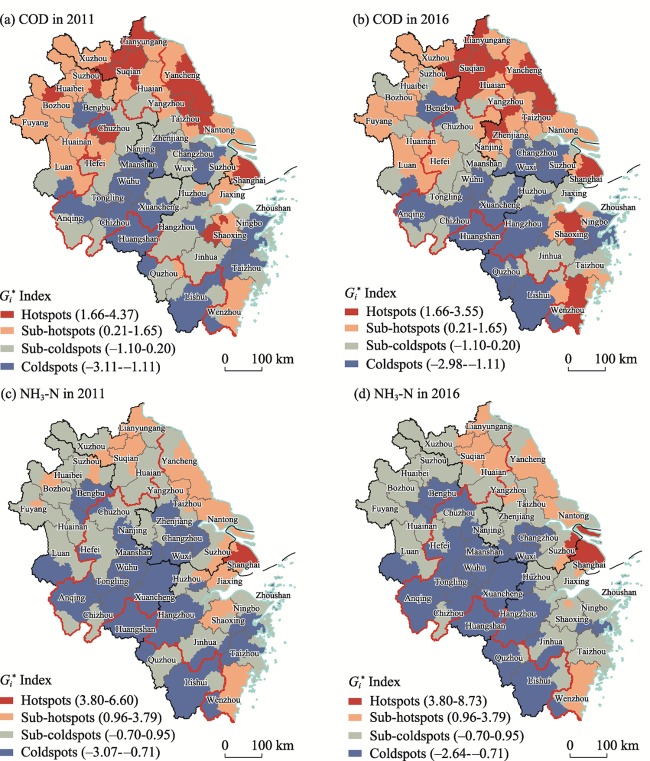
Figure 4 Hot spots of water pollutant discharge intensity at the county level in the Yangtze River Delta (a. chemical oxygen demand (COD) in 2011; b. COD in 2016; c. ammonium-nitrogen (NH3-N) in 2011; d. NH3-N in 2016)

3.2 Estimation of drivers

Given the significant spatial correlations of COD and NH3-N discharges in the YRD, the use of Ordinary Least Squares (OLS) estimation would produce obvious bias, so an econometric model that takes spatial effects into account should be used for driver estimation. The spatial correlation test demonstrated the likelihood that Lagrange Multiplier lag (LM-Lag) and Lagrange Multiplier error (LM-Error) tests were significant, with spatial lag and spatial error effects. The robust LM-Lag and robust LM-Error tests indicated that the SEM model generally fits better than the SLM model from 2011 to 2016. Moreover, the SEM model had smaller values of the Akaike Information Criterion (AIC) and Schwarz Criterion (SC), and the R2 values and logL values of the SEM model were larger than those of the SLM model, further indicating that the SEM model fits better. The variance inflation factor (VIF) was less than 10, indicating that there was no redundancy or multicollinearity among the drivers. Given these results, the SEM model was chosen for quantitative estimation, and the SLM model was used to assist in observing the spatial spillover effect.
Table 3 Results of the spatial correlation tests
Test indicators Chemical oxygen demand Ammonium-nitrogen
2011 2016 2011 2016
Statistics Probability Statistics Probability Statistics Probability Statistics Probability
Moran’s I (error) 0.385 0.000 0.273 0.000 0.384 0.000 0.196 0.000
LM-lag 36.545 0.000 34.502 0.000 36.786 0.000 18.034 0.000
Robust LM-lag 5.547 0.019 8.728 0.003 4.415 0.036 3.539 0.060
LM-error 98.779 0.000 49.791 0.000 98.097 0.000 25.616 0.000
Robust LM-error 67.781 0.000 24.017 0.000 65.727 0.000 11.121 0.001
The SEM model estimation results based on the R Studio platform (Table 4) showed that POP, UR, PGDP, and FAI all passed the 1% significance test, demonstrating that these four indicators produced stable and significant promoting effects on water pollutant discharges from 2011 to 2016. The effect of POP was the most obvious, with the elasticity coefficients of lnPOP in the SEM(COD) and SEM(NH3-N) models for 2016 being 0.904 and 0.851, respectively, indicating that every 1% increase in resident population size will cause an increase of 0.904% and 0.851% in county COD and NH3-N. This demonstrates that resident population size was the main controlling driver affecting the water pollutant discharge in the YRD counties at that time. UR drove water pollutant discharges to the second highest degree, with each 1% increase in urbanization rate in 2016 driving 0.587% and 0.516% increases in county COD and NH3-N, respectively. The elasticity coefficients of lnPGDP for COD and NH3-N discharges and lnFAI for COD and NH3-N discharges were 0.076 and 0.077, and 0.190 and 0.211, respectively, indicating the promoting effects of economic development level and capital investment on water pollutant discharges in the same period.
Table 4 Tests and parameter estimation of the spatial lag model (SLM) and spatial error model (SEM)
Variable SLM (COD) SEM (COD) SLM (NH3-N) SEM (NH3-N)
2011 2016 2011 2016 2011 2016 2011 2016
lnPOP 0.915*** 0.756*** 0.987*** 0.904*** 0.893*** 0.738*** 0.953*** 0.851***
(16.251) (10.510) (19.320) (12.628) (18.168) (10.729) (21.345) (12.451)
lnUR 0.097 0.507*** 0.103 0.587*** 0.122* 0.431*** 0.152** 0.516***
(1.337) (7.494) (1.366) (7.780) (1.939) (6.691) (2.319) (7.269)
lnPGDP 0.244** 0.060** 0.371*** 0.077*** 0.194*** 0.072*** 0.277*** 0.077***
(4.800) (2.351) (6.867) (2.599) (4.429) (2.895) (5.887) (2.742)
lnIS 0.329*** 0.099 0.292*** 0.276*** 0.012 −0.153** 0.033 −0.051
(5.181) (1.498) (4.676) (3.840) (0.218) (−2.479) (0.601) (−0.748)
lnFAI 0.079 0.292*** 0.068 0.190*** 0.056 0.252*** 0.098** 0.211***
(1.423) (4.298) (1.278) (2.589) (1.216) (3.854) (2.122) (2.976)
lnFDI −0.094*** −0.092*** −0.076** −0.037 −0.072** −0.076*** −0.085*** −0.060*
(−3.584) (−3.346) (−2.174) (-1.074) (-3.173) (−2.863) (−2.845) (−1.895)
lnFD −0.231*** −0.378*** −0.184** −0.313*** -0.005 −0.142** −0.010 −0.111
(−3.487) (−5.088) (−2.424) (−3.693) (−0.089) (−1.982) (−0.155) (−1.392)
Spatial lag term (ρ) 0.187*** 0.211*** 0.199*** 0.177***
(6.023) (5.791) (5.993) (4.188)
Spatial error term (λ) 0.621*** 0.482*** 0.616*** 0362***
(13.119) (7.739) (11.897) (5.186)
R2 0.643 0.518 0.736 0.559 0.711 0.588 0.778 0.606
logL −196.091 −228.885 −165.174 −216.408 −156.995 −222.573 −127.067 −221.332
AIC 410.181 475.770 346.348 448.815 330.708 463.146 270.135 452.261
SC 443.664 509.253 376.111 478.578 364.191 496.629 299.897 482.023

Note: *** p<0.01, ** p<0.05, * p<0.1, t-statistics in parentheses.

In addition to the steady drive of water pollution discharge in the YRD by the common drivers mentioned previously, the IS, FDI, and FD had some variability in their influences during 2011-2016, which can be characterized as follows: IS only had a stable effect on COD discharges in the county (p<0.01), while it was not significant for NH3-N discharges. Each 1% increase in the share of secondary industry led to 0.292% and 0.276% increases in COD in 2011 and 2016. This mainly revealed the differences in the source structure of different water pollutants; the share of industrial sources in the YRD for all types of COD discharge remained at approximately 20%, while the NH3-N discharge share of industrial sources was relatively low. This was shown by the scatter plot of the county industrial source discharge share intensity (Figure 5). COD had more counties with a greater than 20% share of industrial source discharges (95) than did NH3-N (29). It also reflected that IS was significantly pulling on the high-intensity COD discharge counties. FDI passed the test in the SEM(COD) model in 2011 and in the SEM(NH3-N) model in 2011 and 2016; its elasticity coefficient was in the range of −0.09 to −0.06, reflecting that foreign capital had a weak inhibitory effect on water pollutant discharges. FD was only significant in the SEM(COD) model, and the elasticity coefficient decreased from −0.184 in 2011 to −0.313 in 2016, indicating that the inhibitory effect of FD on COD discharges had increased.
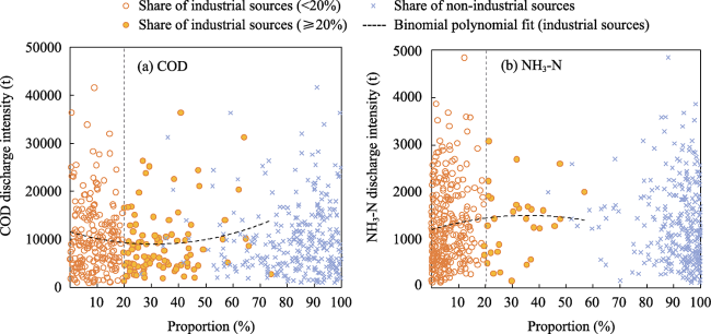
Figure 5 Scatter plot of discharge share of industrial source and discharge intensity at the county level
It should be noted that the spatial lag term (ρ) of each model during 2011-2016 was in the range of 0.17-0.22, and the spatial error term (λ) was in the range of 0.36-0.63, and all variables have passed the 1% significance test. Water pollutant discharge in the counties of the YRD was significantly influenced not only by local drivers but also by the discharge of neighboring counties, meaning that there was an obvious spatial spillover effect. This might be a commonality between local and neighboring areas in terms of industrial structure, production costs, and markets. Under the combined effect of the economic division of labor system, consumer preferences, and logistics costs, if local pollution-intensive industries were difficult to clean up, water pollutant discharges from neighboring areas were also positively driven. Moreover, the error shocks from the above-unconsidered influences could show a certain degree of spatial spillover effects on adjacent county discharges, such as spatial errors in the transfer of pollution-intensive industries to neighboring areas and differences in environmental policies in adjacent counties.

3.3 Diagnosis of scale effects and their spatial heterogeneity

3.3.1 Scale effects

Compared with the SLM, SEM, and GWR models, the MGWR model can take into account the spatial roughness of different factors in driving water pollution discharge through the optimal bandwidth, so the MGWR model was constructed to further analyze the scale effects of the drivers. A comparison of the performance of MGWR and GWR for COD and NH3-N is given in Table 5. The R2 of the MGWR models were 0.649 for COD and 0.683 for NH3-N, which were significantly better than those of the two GWR models, and the AICc values were 592.088 and 556.884, which were also lower than the results of the GWR models. The MGWR model outperformed the GWR model in diagnosing the scale effects and spatial heterogeneity because it took the scale diversity of the drivers into account and reduced a large amount of noise and bias in the regression coefficients to enhance the model robustness.
Table 5 Comparison of model performance of Geographically Weighted Regression (GWR) and Multiscale Geographically Weighted Regression (MGWR)
Indicator GWR (COD) MGWR (COD) GWR (NH3-N) MGWR (NH3-N)
R2 0.597 0.649 0.657 0.683
AICc 625.636 592.088 579.324 556.884
RSS 110.933 94.264 93.571 86.361
The bandwidths of the different drivers in the GWR and MGWR models are given in Table 6. The bandwidths of GWR (COD) and GWR (NH3-N) were 155 and 89, accounting for 50.82% and 29.18% of the total sample, while the MGWR model reflected the bandwidth differences of each driver and revealed distinct scale effects. Based on the bandwidth weight of the global sample (BW) and the corresponding administrative district width, the drivers could be classified into two levels of scale effects; the macro or global scale (BW>50%) and the micro or local scale (BW≤50%). In the MGWR (COD) model, the bandwidths of PGDP, UR, and POP were above 297 and the BWs were above 90%, which could be regarded as global-level drivers, while the bandwidths of IS, FAI, and FD were 140, 116, 95, and the BW values were less than 50%, which meant they were local-level drivers; there was a high degree of spatial nonstationarity in the effects of these drivers. In the MGWR (NH3-N) model, there was also some spatial heterogeneity in the drivers that had significant effects on NH3-N discharges, with UR and POP being global-level drivers, while the other factors were local-level drivers.
Table 6 Bandwidths of drivers estimated by the Multiscale Geographically Weighted Regression (MGWR) model
Variable MGWR (COD) Variable MGWR (NH3-N)
Bandwidth Percentage (%) Indicative scale Bandwidth Percentage (%) Indicative scale
lnPOP 297 97.38 Global lnPOP 178 58.36 Global
lnUR 304 99.67 Global lnUR 304 99.67 Global
lnPGDP 304 99.67 Global lnPGDP 51 16.72 Local
lnIS 140 45.90 Local lnFDI 75 24.59 Local
lnFAI 116 38.03 Local lnFAI 137 44.92 Local
lnFD 95 31.15 Local GWR bandwidth 89 29.18
GWR bandwidth 155 50.82

3.3.2 Spatial heterogeneity

The regression coefficients measured by MGWR were visualized, and the spatial distributions are shown in Figures 6 and 7. In particular, the counties with insignificant regression coefficients (p>0.1) among the drivers, as determined by Pseudo t test, are shaded with slanted lines indicating that the analyzed drivers were weakly explanatory in that county (Fotheringham et al., 2017).
(1) Global drivers: The global drivers of water pollutant discharges in the YRD included UR, POP, and PGDP. The global drivers were characterized by strong effects and low spatial heterogeneity. The specific effects and their spatial effects are given in what follows.
The regression coefficients of POP on COD and NH3-N were significantly positive in the whole region, with coefficient value intervals ranging from 0.624 to 0.710 and 0.391 to 0.750 and standard deviations of 0.030 and 0.122. These results indicated that the size of the population as a global variable was prominently driven by high intensity and low spatial heterogeneity. That is, a higher population size would generally increase the base of residential water pollutant discharges, leading to a significant growth in county water pollutant discharges. It should be noted that, unlike the higher spatial smoothness of COD (Figure 6a), the effect of population size on NH3-N discharges increased from the Taihu Lake and Hangzhou-Jiaxing-Huzhou-Ningbo areas to the periphery (Figure 7a), among which all of Anhui and the northern part of Jiangsu are more affected. Therefore, guiding residents to a greener lifestyle with lower discharges, energy consumption, and pollution will reduce the intensity of water pollutant discharges per unit of population and be beneficial to the regional water pollution trend in the YRD.
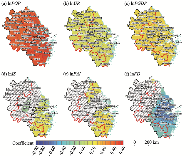
Figure 6 Spatial distribution of regression coefficients of chemical oxygen demand discharge drivers in the Yangtze River Delta (a. lnPOP; b. lnUR; c. lnPGDP; d. lnIS; e. lnFAI; f. lnFD)
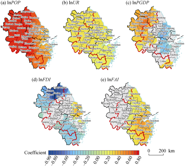
Figure 7 Spatial distribution of regression coefficients of NH3-N discharge drivers in the Yangtze River Delta (a. lnPOP; b. lnUR; c. lnPGDP; d. lnFDI; e. lnFAI)
The regression coefficients of UR on COD and NH3-N were significantly positive regionwide, with coefficient value intervals ranging from 0.189 to 0.206 and 0.243 to 0.281, respectively, and standard deviations of 0.004 and 0.012. This reflected the promoting effect of urbanization level and low spatial heterogeneity. From Figure 6b and Figure 7b, it can be seen that the regression coefficients of urbanization on COD and NH3-N are also slightly higher in western Anhui, western Zhejiang, and northern Jiangsu, which are located on the periphery of urban agglomerations and have relatively low urbanization levels compared with the central areas. Thus, against the background of rapid urbanization in the YRD, it is necessary to focus not only on the water pollution treatment facilities in metropolitan areas and large cities but also on the construction of pollution treatment facilities and pipeline networks in small and medium-sized cities, counties, and even towns.
The regression coefficients of PGDP on COD were significantly positive across the region, with coefficient values ranging from 0.265 to 0.287 and a standard deviation of only 0.006. These results indicated that the level of economic development has a strong promoting effect on COD discharges, and there is almost no spatial heterogeneity, and this driver almost had equal impacts on COD discharges in all counties of the YRD(Figure 6c). In contrast, the level of economic development on NH3-N discharges was only locally significant, with higher levels of economic development in the Suzhou-Wuxi-Changzhou and Hangzhou metropolitan areas showing an inhibitory effect, and higher levels having a facilitating effect in the Hefei metropolitan area and fringe areas of urban agglomerations (Figure 7c). Thus, the companion effect between COD discharges and economic development levels in the YRD and the promoting effect of NH3-N discharges in counties with economic development levels below 43,769.23 RMB show that it is still necessary to change the development mode at the expense of the water environment and pay attention to the cost of water pollution control and water environment benefits in economic growth drivers. A high-quality economic development pattern that is compatible with the carrying capacity of the water environment should be promoted.
(2) Local drivers: The local drivers of water pollutant discharges in the YRD included IS, FDI, FAI, and FD. As shown in Figure 8, this category of drivers was characterized by strong spatial heterogeneity and large differences in the driving intensity of different water pollutants. The specific effects and their spatial effects are given in what follows.
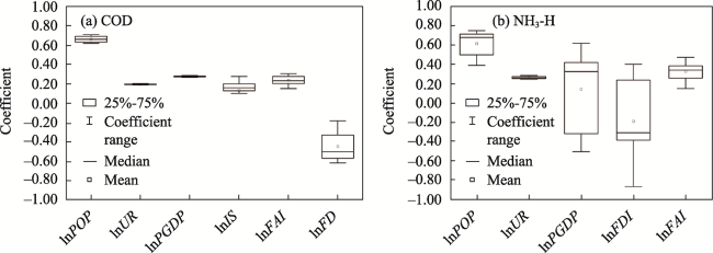
Figure 8 Box plot of regression coefficients for drivers of water pollutant discharges
The regression coefficients of IS on COD were locally significant and usually positive, with coefficient values ranging from −0.124 to 0.276, with a mean of 0.132 and a standard deviation of 0.115. This reflected that the level of industrialization is a local increase driver of COD. As shown in Figure 6d, further statistics combining the industry output value and COD discharge shares of various manufacturing industries revealed that in the Shanghai metropolitan area, the Suzhou-Wuxi-Changzhou metropolitan area, and most of Zhejiang, the concentration of COD pollution-intensive manufacturing industries is high. Such a high concentration would cause the effect of the level of industrialization on COD discharges to remain driven by an elasticity coefficient of 0.2 or more. The industrialization path of the central area of the YRD with high water consumption and high pollution discharge still needs to be shifted. This will continuously guide the COD pollution-intensive manufacturing industries to eliminate outdated process equipment and strengthen the production transformation to clean technology.
The regression coefficients of FDI on NH3-N were locally significant, with coefficient values ranging from −0.875 to 0.402, means and standard deviation of −0.197 and 0.372. This indicated that FDI, as a local variable, had a bidirectional effect and strong spatial heterogeneity on NH3-N discharges in the county. As shown in Figure 7d, FDI was positively driven by NH3-N discharges in Shanghai, Suzhou, Nantong, Jiaxing, Ningbo, Zhoushan, and other cities in the center of the urban agglomerations, showing that the riverside and seaside locations were still favored by foreign investors in ammonia and nitrogen pollution-intensive industries. Conversely, the inhibitory effect of FDI was particularly evident in the peripheral areas of the urban agglomerations, such as northern Jiangsu, northern Anhui, and southern Zhejiang, where the phenomenon of multinational companies seeking pollution refuge in the YRD had significantly improved as stricter environmental disposal standards, discharge restrictions, and other environmental access thresholds were set for foreign enterprises.
The regression coefficient values of FAI on COD and NH3-N ranged from 0.150 to 0.304 and 0.145 to 0.474, with standard deviations of 0.040 and 0.084, respectively. This reflected the local promoting effect of FAI on the two types of water pollutant discharges. In terms of spatial heterogeneity, the spatial sensitivity on NH3-N discharge was stronger than that on COD discharge. The FAI in the YRD was in the form of capital construction investment, renewal and renovation investment, and real estate development investment. A large quantity of investment flowing to high energy-consuming and high discharge industries creates a promotional effect on water pollutant discharges, which is particularly prominent in Hangzhou, Jiahu, and coastal cities (Figures 6e and 7e). Thus, there is an urgent need to promote the structural transformation of FAI in the future and to facilitate the shift from end-of-pipe disposal investment to source-process-end-of-pipe treatment investment. The share of investment in environmental infrastructure construction, discharge treatment, and application of discharge reduction technologies should be compulsorily enforced, and the transformation of investment structure should be forced by the assessment of the environmental benefits of an investment.
The regression coefficients of FD on COD were locally significant and usually negative, with coefficient values ranging from −0.618 to 0.230 and a mean of −0.446 and a standard deviation of 0.154. This reflected the strong spatial heterogeneity and inhibitory effect of local fiscal autonomy on COD discharges. In the context of the current fiscal decentralization system, the increased degree of fiscal decentralization gives local government greater authority over matters and funds (Li et al., 2005; Shen et al., 2005). When local environmental awareness is increased and top-down environmental constraints become stronger, local governments will have the ability and willingness to raise local environmental access thresholds and enforce environmental regulations (Xu et al., 2017; Zhang et al., 2017; Bo et al., 2018). As shown in Figure 6f, FD had an obvious dampening effect on COD discharges within the urban agglomeration centers, indicating to some extent the meritocratic effect of local governments in implementing environmental regulations.

4 Conclusion and discussion

This paper adopts SEM, SLM, and an improved MGWR model to quantitatively estimate the drivers and scale effects of water pollutant discharges, which are of certain scientific value to deeply analyze the environmental effects of urban agglomeration formation and development. This study can provide a basis for formulating countermeasures to reduce water pollutants in urban agglomerations in the context of rapid urbanization and industrialization. The four main conclusions and discussions are as follows:
(1) Urban agglomerations were characterized by large water pollutant discharges, high discharge intensity, and strong spatial spillover. The YRD carries 17.69% of the COD and 19.08% of the NH3-N discharges in China, with 4% of the national land space. The estimation results of the SEM and SLM models showed that POP, UR, PGDP, and FAI have significant promoting effects on water pollutant discharges. The distributions of hot zones from 2011 to 2016 and the results of positive and relatively smooth values of spatial lag and error terms reflected the existence of obvious spatial spillover of water pollutant discharges from urban agglomerations, especially in the coastal and riverine zones in the central area of the YRD urban agglomeration, and in the northern Jiangsu Province, which maintain a strong local spatial viscosity.
(2) The MGWR model took the diversity of scales among drivers into account, effectively reduced the noise and bias of regression coefficients, and examined the scale effect of drivers and the spatial heterogeneity of the influence through optimal bandwidths. Empirical studies in the YRD showed that POP, UR, and PGDP were global-level drivers, and the effect of these drivers on water pollutant discharges was relatively stable and spatially widespread. Therefore, with the rapid urbanization of the YRD, it is urgent to guide residents to a greener lifestyle to reduce the base of water pollutant discharges, focusing not only on supporting water pollutant disposal facilities in each metropolitan area within the urban agglomeration center, but also on strengthening the construction of water pollution treatment facilities and pipeline networks in small and medium-sized cities, counties, and even towns. In addition, for the companion effect and global impact between water pollutant discharges and the level of economic development, it is still necessary to change the mode of economic development; the cost of pollution control and environmental costs should be included in a high-quality economic development assessment system. A pattern of socioeconomic development that is compatible with the environmental carrying capacity should also be promoted.
(3) The regression coefficient analysis of MGWR (COD) and MGWR (NH3-N) models found that IS, FAI, FDI, and FD acted mainly at the local level and only influenced water pollutant discharge in local areas; the spatial variation of the intensity of the effect was significant. IS was prominently driven by COD discharges in Shanghai metropolitan area, Suzhou-Wuxi-Changzhou metropolitan area, and Zhejiang Province, reflecting the significant role of COD pollution-intensive manufacturing industries. The local promoting effect of FAI on COD and NH3-N indicated that the YRD needs to further optimize the structure of fixed asset investment, especially in Hangzhou, Jiaxing, Huzhou, and coastal areas where the effect intensity was higher, and explore new investment and financing models that shift from end-of-pipe disposal investment to source-process-end-of-pipe treatment investment. Moreover, the inhibitory effect of FDI on water pollutant discharges was particularly obvious in the marginal areas of urban agglomerations such as northern Jiangsu, northern Anhui, and southern Zhejiang. Thus, in these areas, the technological spillover and demonstration effect of foreign enterprises in total driver productivity and environmental protection production processes should be amplified to effectively reduce the water consumption and pollutant discharges in economic development. FD has a significant inhibitory effect on COD discharges in urban agglomerations, so the development of a local decentralized incentive mechanism that incorporates the weight of pollution reduction and treatment effects is recommended to give full play to the merit-based effect of environmental regulation by local governments through a flexible and differentiated reward and punishment policy system.
(4) The drivers and scale effects of water pollutant discharges show that in the context of ecological conservation and green development, the complex relationship between water pollution management and socioeconomic development has been changed from a zero-sum conflict to a win-win reconciliation by multiple factors such as production structures, lifestyles, social institutions, and values. Future in-depth discussions are needed on the following: Given that POP, UR, and PGDP are global drivers of water pollutant discharges, it is necessary to further reveal the differences and linkages among them at national, provincial, and municipal scales to provide a basis for the design of multilevel and multiscale environmental regulations. The spatiotemporal interactions between water pollution discharge and water environmental quality in transboundary areas of urban agglomerations should be explored to achieve natural ecosystem integrity and high-quality ecological environmental integrations. Based on the spatial coupling characteristics and mechanisms, seek a spatial organization mode of urban agglomerations with better environmental benefits, adjustments to synergistic industrial layouts, and a path to integration of watershed emissions reduction. By enriching the panel data of the study area with various types of pollution source surveys and pollutant discharges estimations, we can analyze the interactions between the scale effects of water pollution discharge drivers and the scale, structure, and technology effects based on a long time-series study. The causes, mechanisms, and spatial effects of capital, fiscal decentralization, and environmental regulation on water pollution-intensive industries can be deeply explored.
[1]
Ahmad M, Jiang P, Majeed A et al., 2021. The dynamic impact of natural resources, technological innovations and economic growth on ecological footprint: An advanced panel data estimation. Resources Policy, 69: 101817.

DOI

[2]
Akca H, Ozturk I, Karaca C, 2012. Economic development and environment pollution in high and middle-income countries: A comparative analysis of environmental Kuznets curve. Actual Problems of Economics, 137(11): 238-249.

[3]
Alimi O S, Budarz J F, Hernandez L M et al., 2018. Microplastics and nanoplastics in aquatic environments: Aggregation, deposition, and enhanced contaminant transport. Environmental Science & Technology, 52(4): 1704-1724.

DOI

[4]
Al-Mulali U, Ozturk I, Lean H H, 2015. The influence of economic growth, urbanization, trade openness, financial development, and renewable energy on pollution in Europe. Natural Hazards, 79(1): 621-644.

DOI

[5]
Anselin L, 1988. Spatial Econometrics:Methods and Models. Netherlands: Springer.

[6]
Bo Wenguang, Xu Wei, Wang Junfeng, 2018. Local government competition and environmental regulation heterogeneity: Race to the bottom or race to the top? China Soft Science, (11): 76-93. (in Chinese)

[7]
Böcher M, 2012. A theoretical framework for explaining the choice of instruments in environmental policy. Forest Policy and Economics, 16: 14-22.

DOI

[8]
Chang Heejun, 2005. Spatial and temporal variations of water quality in the Han River and its tributaries, Seoul, Korea, 1993-2002. Water Air and Soil Pollution, 161: 267-284.

DOI

[9]
Chen J, Xu C, Li K et al., 2018. A gravity model and exploratory spatial data analysis of prefecture-scale pollutant and CO2 emissions in China. Ecological Indicators, 90: 554-563.

DOI

[10]
Cheng Xi, 2012. Study on relationship between water quality change and economic development of Taihu Lake. Environment and Sustainable Development, 37(5): 73-77. (in Chinese)

[11]
Cole M A, Elliott R, Zhang J, 2011. Growth, foreign direct investment, and the environment: Evidence from Chinese cities. Journal of Regional Science, 51(1): 121-138.

DOI

[12]
Cole M A, Neumayer E, 2004. Examining the impact of demographic factors on air pollution. Population and Environment, 26(1): 5-21.

DOI

[13]
Fan Jie, Zhao Yannan, 2021. China’s regional development pattern oriented toward modernization: The scientific connotation and strategic priorities. Economic Geography, 41(1): 1-9. (in Chinese)

DOI

[14]
Fang Chuanglin, 2014. Important progress and future direction of studies on China’s urban agglomerations. Acta Geographica Sinica, 69(8): 1130-1144. (in Chinese)

DOI

[15]
Fang Chuanglin, Wang Zhenbo, Ma Haitao, 2018. The theoretical cognition of the development law of China’s urban agglomeration and academic contribution. Acta Geographica Sinica, 73(4): 651-665. (in Chinese)

DOI

[16]
Fotheringham A S, Yang W, Kang W, 2017. Multiscale geographically weighted regression (MGWR). Annals of the American Association of Geographers, 107(6): 1247-1265.

DOI

[17]
Ghosh J K, Wilhelm M, Su J et al., 2012. Assessing the influence of traffic-related air pollution on risk of term low birth weight on the basis of land-use-based regression models and measures of air toxics. American Journal of Epidemiology, 175(12): 1262-1274.

DOI PMID

[18]
Gong P, Liang S, Carlton E J et al., 2012. Urbanization and health in China. The Lancet, 379(9818): 843-852.

DOI

[19]
Grossman G M, Krueger A B, 1995. Economic growth and the environment. The Quarterly Journal of Economics, 110(2): 353-377.

DOI

[20]
Guo Chenglong, Zhang Zhiguang, 2017. Discussion on environmental Kuznets curve in Yangtze River Delta: Analysis based on Jiangsu, Zhejiang and Shanghai. Science and Technology Management Research, 37(24): 227-233. (in Chinese)

[21]
Hamid I, Alam M S, Murshed M et al., 2021. The roles of foreign direct investments, economic growth, and capital investments in decarbonizing the economy of Oman. Environmental Science and Pollution Research, 29(15): 22122-22138.

DOI

[22]
He J, 2006. Pollution haven hypothesis and environmental impacts of foreign direct investment: The case of industrial emission of sulfur dioxide (SO2) in Chinese provinces. Ecological Economics, 60(1): 228-245.

DOI

[23]
Jiang Wei, Lai Mingyong, 2009. Spatial dependence and FDI location determinants: Spatial econometrical analysis based on Chinese urban data. Finance and Trade Research, 20(6): 1-6. (in Chinese)

[24]
Li H, Zhou L, 2005. Political turnover and economic performance: The incentive role of personnel control in China. Journal of Public Economics, 89: 1743-1762.

DOI

[25]
Li M, Li C, Zhang M, 2018. Exploring the spatial spillover effects of industrialization and urbanization factors on pollutants emissions in China’s Huang-Huai-Hai region. Journal of Cleaner Production, 195: 154-162.

DOI

[26]
Liang L, Wang Z, Li J, 2019. The effect of urbanization on environmental pollution in rapidly developing urban agglomerations. Journal of Cleaner Production, 237: 117649.

[27]
Liao Xianchun, Xia Enlong, 2015. Why China attracts FDI inflows? A perspective of environmental stringency and the degree of corruptibility. World Economy Studies, (1): 112-119, 129. (in Chinese)

[28]
Lu X C, Lin C Q, Li W K et al., 2019. Analysis of the adverse health effects of PM2.5 from 2001 to 2017 in China and the role of urbanization in aggravating the health burden. Science of The Total Environment, 652: 683-695.

DOI

[29]
Luo Gusong, Li Tao, 2019. Dynamic change and driving factors of land use efficiency differences affected by carbon emissions at the provincial level in China. Acta Ecologica Sinica, 39(13): 4751-4760. (in Chinese)

[30]
Morley B, 2012. Empirical evidence on the effectiveness of environmental taxes. Applied Economics Letters, 19(18): 1817-1820.

DOI

[31]
Oshan T M, Li Z, Kang W et al., 2019. MGWR: A python implementation of multiscale geographically weighted regression for investigating process spatial heterogeneity and scale. ISPRS International Journal of Geo-Information, 8(6): 269.

DOI

[32]
Shen Kunrong, Fu Wenlin, 2005. The relationship between China’s decentralized system in finance and her regional economic growth. Management World, (1): 31-39, 171-172. (in Chinese)

[33]
Sheng Bin, Lv Yue, 2012. Impact of foreign direct investment on China’s environment: An empirical study based on industrial panel data. Social Sciences in China, (5): 54- 75, 205-206. (in Chinese)

[34]
Singh P, Kikon N, Verma P, 2017. Impact of land use change and urbanization on urban heat island in Lucknow city, Central India. A remote sensing based estimate. Sustainable Cities and Society, 32: 100-114

DOI

[35]
State Council of the People’s Republic of China (SCPRC), 2019. Outline of the Yangtze River Delta Regional Integrated Development Plan, 2019-12-01. (in Chinese)

[36]
Sun L, Wei J, Duan D H et al., 2016. Impact of land-use and land-cover change on urban air quality in representative cities of China. Journal of Atmospheric and Solar-Terrestrial Physics, 142: 43-54.

DOI

[37]
Tasdighi A, Arabi M, Osmond D L, 2017. The relationship between land use and vulnerability to nitrogen and phosphorus pollution in an urban watershed. Journal of Environmental Quality, 46(1): 113-122.

DOI PMID

[38]
Ulucak R, Khan S U D, Baloch M A et al., 2020. Mitigation pathways toward sustainable development: Is there any trade-off between environmental regulation and carbon emissions reduction? Sustainable Development, 28(4): 813-822.

DOI

[39]
Wang D W, Li J, 2020. Coastal haze pollution, economic and financial performance, and sustainable transformation in coastal cities. Journal of Coastal Research, 109: 1-7.

[40]
Wang X, Tian G, Yang D et al., 2018. Responses of PM2.5 pollution to urbanization in China. Energy Policy, 123: 602-610.

DOI

[41]
Wen Guanzhong, Chai Yi, 2015. Government-led urban land use efficiency: Empirical results from China. Academic Monthly, 47(1): 11-23. (in Chinese)

[42]
Wolf L J, Oshan T M, Fotheringham A S, 2018. Single and multiscale models of process spatial heterogeneity. Geographical Analysis, 50(3): 223-246.

DOI

[43]
Xu Hui, Yang Ye, Nie Du, 2017. Influence path of fiscal decentralization on environmental pollution in top ten urban agglomerations in China. Urban Problems, (6): 14-24. (in Chinese)

[44]
Yao Shimou, Zhou Chunshan, Wang De et al., 2016. New Perspectives on Urban Agglomerations in China. Beijing: Science Press. (in Chinese)

[45]
Yu H, Fotheringham A S, Li Z et al., 2020. Inference in multiscale geographically weighted regression. Geographical Analysis, 52(1): 87-106.

DOI

[46]
Zhang Hua, Feng Chao, Liu Guanchun, 2017. Chinese style environmental federalism: A study on the effect of environmental decentralization on carbon emissions. Journal of Finance and Economics, 43(9): 33-49. (in Chinese)

[47]
Zhou Jieqi, Xia Nanxin, Liang Wenguang, 2019. FDI, independent innovation and haze pollution: Evidence from China. R&D Management, 31(2): 78-90. (in Chinese)

[48]
Zhou Kan, Li Hui, Shen Yuming, 2020. Spatiotemporal patterns and driving factors of environmental stress in Beijing-Tianjin-Hebei region: A county-level analysis. Acta Geographica Sinica, 75(9): 1934-1947. (in Chinese)

DOI

[49]
Zhu Y G, Ioannidis J P A, Li H et al., 2011. Understanding and harnessing the health effects of rapid urbanization in China. Environmental Science & Technology, 45(12): 5099-5104.

DOI

Outlines

/