Research Articles

Measuring Chinese cities’ economic development with mobile application usage

  • LIU Zhewei , 1, 2 ,
  • LIU Jianxiao , 3, * ,
  • HUANG Xiao 4 ,
  • ZHANG Erchen 5 ,
  • CHEN Biyu 2, 6, 7
Expand
  • 1. Smart Cities Research Institute, Department of Land Surveying and Geo-informatics, The Hong Kong Polytechnic University, Hung Hom, Hong Kong, China
  • 2. State Key Laboratory of Information Engineering in Surveying, Mapping and Remote Sensing, Wuhan University, Wuhan 430079, China
  • 3. Department of Real Estate and Construction, Faculty of Architecture, The University of Hong Kong, Hong Kong, China
  • 4. Department of Geosciences, University of Arkansas, AR, USA
  • 5. Independent Researcher
  • 6. Collaborative Innovation Center of Geospatial Technology, Wuhan University, Wuhan 430079, China
  • 7. Geocomputation Center for Social Sciences, Wuhan University, Wuhan 430079, China
* Liu Jianxiao, specialized in urban planning and urban informatics. E-mail:

Liu Zhewei, PhD, specialized in smart cities and spatial big data analytics. E-mail:

Received date: 2022-01-07

  Accepted date: 2022-06-09

  Online published: 2022-12-25

Supported by

Wuhan University State Key Laboratory of Information Engineering in Surveying Mapping and Remote Sensing(21S02)

Abstract

With the rise of smart phones, mobile applications have been widely used in daily life. However, the relationship between individuals’ mobile application usage and cities’ economic development has yet to be investigated. To study this question, this work utilizes a dataset containing users’ history of mobile application usage records (MAURs) and investigates how MAURs are related to Chinese cities’ economic development. Our analysis shows the cities’ GDP and number of MAURs are highly correlated, and at the individual level, people in wealthier cities (higher GDP per capita) tend to have more active mobile application usage (MAURs per capita). The results also demonstrate the relevance between cities’ GDP and MAURs varies significantly among different demographic groups, with male users’ relevance consistently higher than female users’ and working-age people’s relevance higher than other age groups. A boosted tree regression model is then applied to predict cities’ GDP with MAURs and proves to achieve high goodness-of-fit (over 0.8 R-square) and good prediction accuracy, especially for the economically developed and populous regions in China. To the best of our knowledge, this is the first time that the relationship between MAURs and cities’ economic development is revealed, which contributes to novel knowledge discovery for regionalization and urban development.

Cite this article

LIU Zhewei , LIU Jianxiao , HUANG Xiao , ZHANG Erchen , CHEN Biyu . Measuring Chinese cities’ economic development with mobile application usage[J]. Journal of Geographical Sciences, 2022 , 32(12) : 2415 -2429 . DOI: 10.1007/s11442-022-2054-x

1 Introduction

The recent rise of big data has provided researchers with novel data sources and tools to study unexplored issues before (Dong et al., 2019; Liu et al., 2021). In relevant fields, various kinds of new big data have been introduced to address issues such as inferring socioeconomic indicators (Gamma et al., 2016; Mellander et al., 2015), study of social networks (Palla et al., 2007; Park et al., 2018), human mobility (Gonzalez et al., 2008; Blumenstock, 2012), pandemic transmission (Kraemer et al., 2020; Tian et al., 2020; Shi et al., 2021).
Among various kinds of big data, the mobile phone data is a very popular data source. One commonly-used type of mobile phone big data is call detail records (CDR), which tracks users’ approximate locations and the calling/receiving parties when they make a call/message (Blumenstock et al., 2015). Another type related to mobile phone big data is users’ log recorded in a single application, which may track individuals’ movement trajectories or search history in that single application (Dong et al., 2017; Sun et al., 2017).
However, a limitation of above mobile phone data (i.e., CDR and records from a single application) is that these records are far incapable of indicating individuals’ overall usage of all the installed applications on the phone. Dozens of mobile applications may be installed on a smart phone, and daily used by users for different purposes, like working, communication and entertainment. Due to the data availability issue, such records of individuals’ overall mobile application usage on the phone have seldom been accessed or used in socioeconomic studies. Moreover, the individual’s mobile application usage is a reflection of his/her activity in the online virtual cyber world. Whether people’s online behaviours in the virtual world will be affected by the social wealth of the physical world that they live in? Whether the society’s economic development can be inferred from the residents’ mobile application usage? These meaningful questions can add more knowledge into the human dynamics under the compound influence of physical and virtual worlds, yet remain unsatisfactorily addressed.
Consequently, to answer the above questions, this work utilizes a dataset containing users’ history of mobile application usage (detailed information about “who used what application at when and where”), and investigates the relationships between individuals’ mobile application usage records (MAURs) and the city-level economic development. Specifically, in our work, the number/frequency of the mobile application usage is used to quantify the MAURs (e.g., if an individual has used the apps on the phone 100 times during the experimental period, the individual’s MAURs is then 100). Our results demonstrate the high correlation between cities’ economic development and MAURs, and also the correlation variation among different demographic groups. A boosted tree model is then applied for regression and demonstrate the model’s effectiveness and accuracy in predicting cities’ economic development with MAURs.
The detailed contributions of this work can be summarized as below:
• For the first time, we reveal the correlation between individuals’ mobile application usage and cities’ economic development. Our findings show that (1) people in wealthier cities tend to have more active mobile application usage; (2) the relevance of male and work-age users’ MARUs to GDP, is consistently higher than that of other demographic groups.
• We apply a boosted tree regression model to predict cities’ GDP with MARUs and prove that the regression model can predict cities’ GDP with high goodness-of-fit and accuracy, especially for the economically developed and populous regions.
The rest of this paper is organized as below. Section 2 briefly reviews the previous related work. Section 3 describes our experiment dataset and methodology in details. Section 4 gives our experiment results and important findings. Finally, Section 5 concludes the whole paper and discusses the limitations of this work.

2 Related work on measuring the socioeconomic attributes with big data

The recent expansion of big data collection has profoundly influenced the socioeconomic research (Einav and Levin, 2014; Varian, 2014). Various kinds of newly available big data have been employed in different studies, for measuring socioeconomic statistics and economic activity.
One popular data source used by previous studies is the night-time light satellite image, which has the following advantages: (1) easy access to information; (2) high spatial resolution; and (3) wide geographic coverage (Donaldson and Storeygard, 2016), and thus has been widely used as proxy for socioeconomic variables (Mellander et al., 2015). For instance, Henderson et al. (2012) developed a framework that uses night-time satellite data to complement existing income growth measures, which can be particularly useful for countries with poor-data regions. A similar work was done by Chen and Nordhaus (2011), who examined night-time data as a measurement for GDP and demonstrated its value for countries with low-quality statistics. Night-time light’s capabilities to timely measure socioeconomic status also make it a useful tool for monitoring social disturbance, resulting from natural disasters (Li et al., 2018; Qiang et al., 2020) or man-made humanitarian crises (Li et al., 2014). Nevertheless, the unavailability of long-term, temporally consistent and spatially precise data may potentially undermine the valid application of night-time light (Gibson et al., 2020).
The vast volume of human-generated electronic records has also been applied for measuring socioeconomic outcomes. Sobolevsky et al. (2017) used bank card transactions to predict a series of socioeconomic indexes related to life quality. Related studies also used individual’s web-based search records to forecast various economic indicators, such as consumer confidence, unemployment, crime, and revenue forecast (Ettredge et al., 2005; Choi and Varian, 2012; Gamma et al., 2016; Dong et al., 2017). Another popular data source for measuring economy is social media data (with or without geolocation), which has been used for studying problems like labour market flow and business establishments (Antenucci et al., 2014; Llorente et al., 2015; Glaeser et al., 2017).
Besides the aforementioned kinds of datasets, mobile phone usage is widely used as well for socioeconomic studies. A unique characteristic of mobile phone data is that call detail records (CDR) can record both the spatiotemporal and calling/receiving information of users, which enables the reconstruction of individual’s spatiotemporal trajectories and communication networks. Blumenstock et al. (2015) predicted the individuals’ wealth and possession of different assets, using their history of mobile phone usage. Eagle et al. (2010) quantified the diversity of individuals’ social relationships with users’ mobile phone contacts and demonstrated its strong correlation with communities’ economic development. Researchers further proved the applicability of mobile phone big data in indicating different socioeconomic indicators, including unemployment rates, per capita income and deprivation index (Toole et al., 2015; Almaatouq et al., 2016; Pappalardo et al., 2016). A comparison of the advantages and disadvantages of different data sources for measuring socioeconomic status has been given in Table 1.
Table 1 Advantages/disadvantages of different data sources for measuring socioeconomic status
Data Sources Easy
access
High
spatial
resolution
Wide
geographic
coverage
Indicating
individual
activity
Indicating
human
mobility
Indicating
social
network
Satellite image
Bank card transaction
Web-based search records
Social media
Mobile phone call detail records (CDR)
However, most previous studies using mobile phone big data, utilized the CDR to identify human movement or communication networking. Few works have ever accessed the records of individuals’ overall mobile phone application usages. Whether people’s behaviours in the online virtual world will be affected by the wealth of the physical world? Whether the cities’ economic development can be inferred from the residents’ mobile application usage? These worthwhile research questions remain to be answered.

3 Study dataset and methodology

3.1 Study dataset and preprocessing

This study aims to investigate the relationship between mobile application usage and city’s economic development. Consequently, two kinds of datasets are used for experiments: mobile application usage records (MAURs) and statistic data of cities. The mobile application usage records are from an open-sourced dataset (TalkingData, 2016), published by TalkingData, China’s largest third-party mobile data platform (TalkingData, 2020). The dataset was collected via TalkingData software development kit (SDK) integrated in the mobile applications. When a user uses an application that implements TalkingData SDK, an event will be logged, with spatiotemporal and application information indicating when and where the event is, and what mobile application is used. The geographical coverage of the dataset is in China mainland (without Hong Kong, Macau and Taiwan), and the time period of the dataset is May 1-7, 2016. Users’ age and gender information were also provided in the dataset, with users’ full consents and all personal identifications anonymized for privacy. A detailed dataset description can be found in TalkingData (2016). As the event locations are in the form of coordinates, we employ Baidu Map API for reverse geocoding to retrieve the city where events occurred. After data preprocessing, 3,252,950 events generated by about 60,865 users are recorded in total.
For indicators of economic development, the city’s GDP and GDP per capita are retrieved from the Chinese City Statistical Yearbook 2017. The data of 330 Chinese cities is collected and those cites without available statistics data are excluded from this study. The key attributes of our datasets are summarized as Table 2.
Table 2 Attributes of the experimental datasets
Attributes of mobile application usage Attributes of city’s economic development
Fields Descriptions Fields Descriptions
e_id An id uniquely indicating an event that a mobile application is used city_name The name of a city
app_id An id uniquely indicating an application used in the event population The population of a city
u_id An id uniquely indicating the user of the event GDP The GDP of a city
timestamp The timestamp of the event GDP per capita The GDP per capita of a city
location The location of the event
u_gender The gender of the user
u_age The age of the user

3.2 Methodology

3.2.1 Pearson correlation and boosted decision tree regression model

To understand the relationship between mobile application usage and city’s economic development, Pearson correlation analysis is performed. The Pearson correlation coefficient is tested at 0.01 significance level.
After correlation analysis, we would like to answer: whether the city’s economic development can be measured or predicted, given its residents’ mobile application usage. Consequently, we split the users into different demographic groups (according to their gender and age) and construct a multi-dimension feature vector by calculating the numbers of MAURs of each demographic group:
$\text { feature_vector }=\left(M A U R_{1}, \text { MAUR }_{2}, \ldots, \text { MAUR } R_{n}\right)$
where MAURi is the number of MARUs of the ith demographic group. A boosted decision tree model is then implemented to predict the city’s economic development with the constructed multi-dimension vectors as input feature. The output score of the boosted decision tree model can be written as:
$F_{t}(x)=\sum_{i=1}^{t} f_{i}(x)$
where x is the input feature and fi(x) is the output score of the ith single regression tree. The boosted decision tree model is an ensemble of regression trees using boosting strategy. Given the ground-truth output score y and t trained trees, the (t+1)th tree to be trained, ft+1(x) aims to fit the dataset {x, rt}, where rt is the residual between y and Ft (x), i.e.:
$r_{t}=y-F_{t}(x)$
The python library XGboost is used for the implemented of boosted decision tree regression. For parameter settings, the hyperparameters are find-tuned using Grid Search (Bao and Liu, 2006).
The performance of model regression is evaluated using the measurement R square (R2) via 5-fold cross-validation approach: the datasets are divided into five random folds, each of which is taken alternatively for testing and the remaining four folds for training, until all the five folds have been used once for testing. The results of five testing folds are then averaged to produce the final evaluation of model’s performance.

3.2.2 Spatial analysis of regression model performance

The performance of our regression model may vary from city to city. The follow-up interesting questions are in which regions the model underperforms or outperforms, and whether the regions where the model underperforms or outperforms tend to spatially aggregate. A spatial analysis of the model’s performance is thus conducted to evaluate whether the model’s performance exhibits any spatial pattern (clustered, dispersed or random), which helps to validate the model’s effectiveness and generalizability across different regions.
The global and local patterns of the model’s performance are investigated with Global Moran’s I (Moran, 1950) and Local Moran’s I (Anselin, 1995). The Global Moran’s I and Local Moran’s I are calculated as:
$\left\{\begin{array}{l}I=\frac{N}{W} \frac{\sum_{i} \sum_{j} w_{i j}\left(x_{i}-\bar{X}\right)\left(x_{j}-\bar{X}\right)}{\sum_{i}\left(x_{i}-\bar{X}\right)^{2}} \\I_{i}=\frac{x_{i}-\bar{X}}{S_{i}^{2}} \sum_{j=1, j \neq i}^{n} w_{i, j}\left(x_{j}-\bar{X}\right)\end{array}\right.$
where I is Global Moran’s I and Ii is the Local Moran’s I for ith unit; N/n is the number of units to be investigated; xi is the target attribute of ith unit (in our study, x stands for the indicator of the model’s performance in the region); $\bar{X}$ is the mean of xi; wij is the spatial weight between ith and jth unit (in our study, the spatial weight is measured using the inverse Euclidean distance between the units); W is the sum of wij; $S_{i}^{2}$ is calculated as $S_{i}^{2}=\frac{\sum_{j=1, j \neq i}^{n}\left(x_{j}-\bar{X}\right)^{2}}{n-1}$.
The value of Global Moran’s I ranges from [-1, 1]. A positive Global Moran’s I value indicates positive spatial autocorrelation (clustered) while negative value indicates negative spatial autocorrelation (dispersed), with corresponding p-value and z-score indicating significance level. Local Moran’s I can indicate the extent of spatial clustering of similar values around the observed unit. The output of Local Moran’s I distinguishes four cluster type: cluster of high values (HH), cluster of low values (LL), high value surrounded by low values (HL), and low value surrounded by high values (LH).

4 Results

4.1 Correlations between cities’ economic development and mobile application usage

We investigate the relationship between cities’ economic development and the mobile application usage, using Pearson correlation. The Pearson’s r is first calculated between the cities’ GDP and the total number of MAURs in the cities (shown in Figure 1). The results show that cities’ GDP are highly positively correlated with the number of MAURs in the cities, with a Pearson’s r = 0.914** at 0.01 significance level. The cities with highest GDP (such as Beijing, Shanghai, Shenzhen, Guangzhou) are also among the top cities with most MAURs.
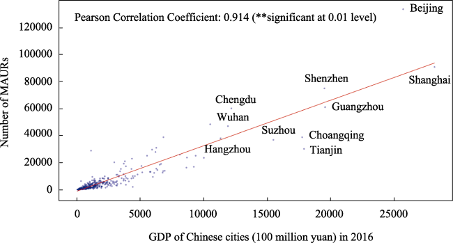
Figure 1 GDP and MAURs of Chinese cities
The total number of MAURs and GDP of a city can be decomposed with the following formula:
$\left\{\begin{array}{c}\text { Total number of MAURs }=\text { Popu } * \text { MAURs per capita } \\G D P=P o p u^{*} G D P \text { per capita }\end{array}\right.$
where Popu is the population of the city. Consequently, an explanation for such high correlation between cities’ GDP and mobile application usage may be that, the cities with more MAURs probably have more residents, thus leading to higher GDP, which means the number of MAURs is a reflection of the population. However, according to the Formula 5, another potential explanation for such high correlation is that, the city’s MAURs per capita and GDP per capita may be positively related, which means people in wealthier cities (higher GDP per capita) may have more frequent/active mobile application usage. Whether the latter explanation is true or not remains an unexplored question.
To investigate the above question, the relationship between cities’ GDP per capita and the average number of MAURs per capita is further studied (Figure 2). In Figure 2, the cities are divided into ten group in terms of their rankings of GDP per capita, and the average numbers of MAURs of every10 thousand people of respective city groups are displayed with boxplot. It shows a clear pattern that the city groups of higher GDP per capita also have higher numbers of MAURs per capita, than city groups of lower GDP per capita. For the top 10% cities in terms of GDP per capita, the median of MAURs number in every 10 thousand people is 35.0; while for the cities in the top 40%-50% and bottom 10%, the medians are 9.1 and 2.8. Our correlation analysis shows the Pearson’s r between cities’ GDP per capita and number of MAURs per capita is 0.789**, with significance at 0.01 level. The above findings demonstrate that people living in wealthier areas (i.e., cities of higher GDP per capita) tend to have more active mobile application usage, than people in less developed areas.
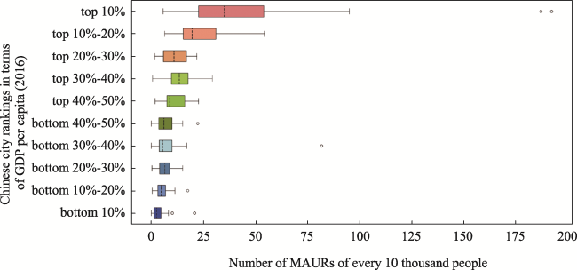
Figure 2 Boxplot of Chinese cities and their numbers of MAURs of every 10 thousand people

4.2 Differentiation among demographic groups

We further divide the users in the dataset into different demographic groups according to their ages and genders (see Table 2), and examine whether the correlation between cities’ GDP and MAURs differentiates among different demographic groups. The results (Figure 3) show that, the Pearson’s r between cities’ GDP and MAURs varies significantly among different groups:
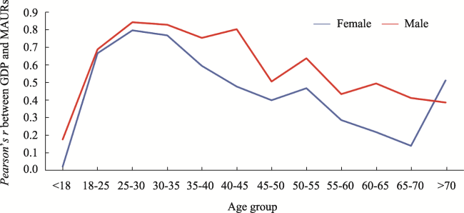
Figure 3 Correlations between cities’ GDP and MAURs of different demographic groups
(1) The relevance of male users’ MARUs to GDP, is consistently higher than that of female users throughout different age groups, with only one age group exception (i.e., over 70 years old);
(2) For both genders, the relevance of MARUs to GDP shares similar trends and the relevance of working age’s (18~60 years old) MARUs to GDP is significantly higher than those of pre-working age (below 18 years old) and post-working age (over 60 years old). The relevance of MARUs to GDP first increases and then decreases as age grows, with the peak achieved at the age group of 25~30 years old (Pearson’s r more than 0.8).
(3) While both genders’ relevance shares similar trends, the range and standard deviation of female users’ relevance are 0.775 and 0.245, larger than those of male users’ relevance (i.e., 0.668 and 0.211), which indicates the relevance of female users’ MARUs to GDP fluctuates and polarizes more than that of male users, across different age groups.

4.3 Inferring cities’ GDP with MAURs and boosted decision tree model

Since the cities’ GDP and MAURs are highly correlated, we then study whether the city’s economic development can be inferred, given its residents’ mobile application usage. The details of the used boosted decision tree model and the input feature are as explained in Equation 1 in Section 3.2.1, and the output of the model is the city’s GDP. In Section 4.2, it has been revealed that the MAURs of different demographic groups may have different correlations with the cities’ GDP. Consequently, the input feature vectors (Equation 1) are constructed based on the MAURs of different demographic groups, which can prevent the information of MAURs of high-correlation groups from the hinderance of low-correlation groups as well as maintain the information of MAURs of low-correlation groups at the same time. The division of demographic groups to construct input feature vectors (Equation 1) is the same as Section 4.2.

4.3.1 Performance of the boosted decision tree model

The performance of our regression model is evaluated using 5-fold cross-validation. Figure 4 presents the predicted GDP and true GDP of 330 Chinese cities investigated in this study. It shows that our tree regression model fits well with the observation and achieves high R2 = 0.805, suggesting our model can explain most proportion of the total variation of the dataset and achieve high goodness-of-fit.
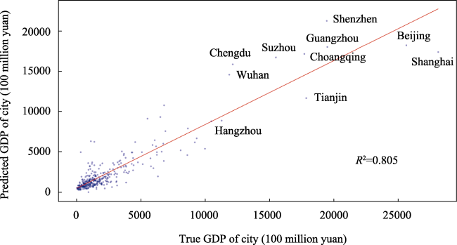
Figure 4 The regression model’s predicted GDP versus true GDP of 330 Chinese cities
However, R2 is a statistic evaluating how well the model fits the overall dataset and yet insufficient to indicate how accurate our model performs on each item (i.e., cities in this study) in the dataset. To measure the accuracy of our model’s prediction of each city’s GDP, we introduce another measurement predictive error (Dong et al., 2019), defined as
$\text { predictive error }=\frac{\mid \text { Predicted GDP }-\text { True GDP } \mid}{\text { True GDP }}$
The predictive error is calculated for each city and used to measure the deviation of predicted GDP from the true GDP of the city. For example, if the regression model achieves 30% predictive error for a city, it means the city’s predicted GDP by the model deviates 30% (lower or higher) from the city’s real GDP. We further calculate the cumulative distribution function of the model’s predictive error as below:
$F(x)=\frac{\sum_{c_{i} \text { error }<x} G D P_{c_{i}}}{\sum_{c_{j}} G D P_{c_{j}}}(0 \leqslant x)$
where the numerator calculates the sum of true GDP of the cities with predictive error less than x, and the denominator calculates the sum of true GDP of all the cities in this study. The cumulative distribution function of predictive error can be used to answer: how much proportion of all the cities’ GDP can be predicted with an error less than a given threshold, and the result is displayed in Figure 5. It shows that the GDP of the cities with predictive error less than 0.30, account for about 60% of the sum of all the Chinese cities’ GDP. About 70% of all the Chinese cities’ GDP, can be predicted with an error less than 0.35. The above results demonstrate that, our model is capable of predicting most Chinese cities’ GDP with good accuracy.
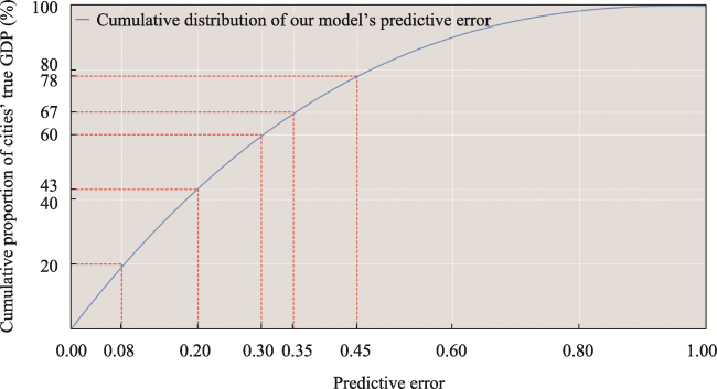
Figure 5 Cumulative distribution of our model’s predictive error

4.3.2 Geographical variation of model’s performance

After evaluation of the model’s overall performance on the whole dataset, the geographical variation of model’s performance over different regions is subsequently investigated. The model’s performance (measured by R2) in several provincial-level regions (hereafter provinces) are displayed in Figure 6. The regression model’s goodness-of-fit varies significantly across different provinces. For example, Hubei shows the highest R2 = 0.962. Guangdong, Jiangsu and Zhejiang also show high R2 around 0.9. In comparison, Liaoning, Qinghai and Xinjiang show relatively low R2 (below 0.6). As the granular unit of this study is in the city level (i.e., the city’s GDP is predicted), the predictive error of each city is mapped in Figure 7 (the cites without available data are excluded). The city-level predictive error shows a similar pattern as the provincial-level R2 analysis. GDP of most Chinese cities can be predicted with high accuracy. The predictive errors of most cities in high-R2 provinces (e.g., Hubei, Guangdong, Jiangsu and Zhejiang) are below 0.35, while for low-R2 provinces (e.g., Liaoning, Qinghai and Xinjiang), the corresponding cities’ predictive errors are largely among a high range (0.35-1).
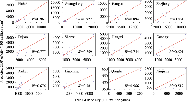
Figure 6 The regression model’s performance over different provincial-level regions of China, measured by R2
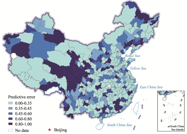
Figure 7 Each city’s predictive error in China (the cites without available data are excluded)
The above results indicate a significant geographical variation of the regression model’s performance over different regions.
Figure 7 shows that the cities with similar predictive errors may be clustered from a visual interpretation. Whether such geographical cluster patterns are statistically meaningful is then investigated, using the spatial autocorrelation analysis (Section 3.2.2). The Global Moran’s I of cities’ predictive errors is 0.069** (significant at 0.01 level), suggesting a positive spatial autocorrelation of cities’ predictive errors, i.e., the cities whose GDP can be accurately predicted by our regression model tend to be near to each other, and vice versa. The Local Moran’s Is (Section 3.2.2) of cities’ predictive errors are further calculated and the four cluster types generated from Local Moran’s I are mapped in Figure 8. It can be seen that the clusters of high predictive errors (HH) are mainly in three regions: Qinghai-Gansu-Sichuan, Heilongjiang, and Liaoning. In contrast, the clusters of low predictive errors are mainly in three other regions: Hebei-Shandong, Anhui-Henan-Huben, Jiangsu-Anhui-Jiangxi.
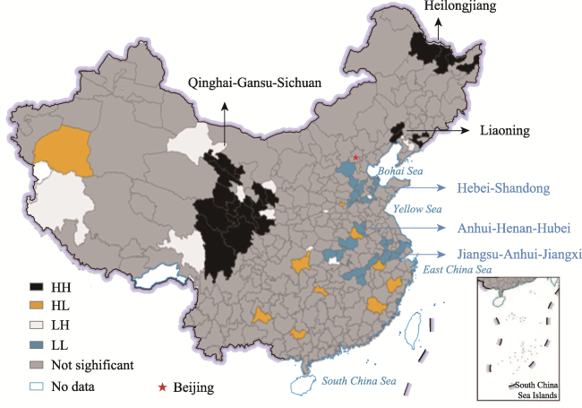
Figure 8 Four cluster types generated from Local Moran’s I of cities’ predictive errors in China
Our above analysis shows that the regression model’s performance varies significantly from place to place, and the places with similar predictive errors tend to be clustered. The regions where the model underperforms are mainly in Northwest (i.e., Xinjiang, Qinghai and Gansu) and Northeast (i.e., Heilongjiang and Liaoning) of China.

4.3.3 Why the model outperforms or underperforms: sensitivity analysis

Sensitivity analysis is conducted here to answer: why the regression model outperforms or underperforms in certain regions. We mainly study the influence of two factors on our model: (1) population, and (2) economic development (GDP). The correlation (Pearson’s r) between cities’ predictive errors and these two factors are investigated, as shown in Table 3.
Table 3 The correlation between cities’ predictive errors and cities’ population and GDP
Population GDP
Pearson’s r with predictive errors -0.235** -0.183**

** significant at 0.01 level, p < 0.01.

It is shown that our model’s predictive errors are negatively correlated with the cities’ population and GDP, which means that the more population and GDP a city has, the more accurately our model can predict its GDP. Such results also echo our previous analysis in Section 4.3.1 and Section 4.3.2, in the following aspects:
• The cumulative distribution function of the model’s predictive error (Figure 5) has shown that for the cities that account for majority of all the cities’ GDP, our model can predict their GDP with a high accuracy. The GDP of cities with high predictive errors only account for a small part of all the cities’ GDP.
• The spatial analysis (Figures 7 and 8) shows the regions with high predictive errors are mainly in Northwest (i.e., Xinjiang, Qinghai and Gansu) and Northeast (i.e., Heilongjiang and Liaoning) of China, which are of relative low ranking in terms of GDP in China. While for the economically developed regions (such as Guangdong, Jiangsu, Zhejiang), our regression model shows high prediction accuracy.
The above results demonstrate our model’s effectiveness and accuracy in predicting Chinese cities’ economic development, especially for the economically developed and populous cities.

5 Discussion

5.1 Implications of the correlation between MAURs and cities’ GDP

Our findings reveal the high correlations between cities’ economic development and MAURs, and that people in wealthier cities (higher GDP per capita) may have more frequent/active mobile application usage. This may be because that the digitization of daily working and lifestyle is easier to achieve high penetration in wealthier cities, where communication infrastructures are more prevalent and residents are more familiar with the information technology, than less developed cities. We also see the relevance of male and work-age users’ MARUs to GDP, is consistently higher than that of other demographic groups, which may reflect the different time distribution and working/living style across different demographic groups.

5.2 Limitations

Admittedly, measuring city’s economic development with MAURs in this work, falls into certain limitations. Firstly, the mechanism underlying the high correlation between MAURs and GDP hasn’t been explained. Though we give our initial assumptions, why people in wealthier cities tend to have more active mobile application usage and why the correlation between MAURs and GDP varies among different demographic groups still need further studies to validate. Secondly, besides population and GDP, the performance of our regression model may be correlated with or even result from other factors, such as cities’ economic and demographic structures. Such correlations or causalities remain to be explored and theoretically explained. Third, the spatial granularity of this study is in the city level. Applying the dataset for indicating socioeconomic status at more fine-grained levels (e.g., street or district level) is a meaningful direction for future work. Fourthly, our study does not differentiate tourists from the local residents in each city. Chances are that the tourists left their home cities and travelled to other cities where MAURs were left during our study periods. Whether the tourists’ application usage patterns differ from those of the local residents and to what degree such differences may affect the results of our analytics, still remain to be evaluated by further studies.

6 Conclusions

Mobile applications have penetrated into almost every aspect of modern lifestyle and drastically changed human-beings’ ways of working, communication, entertainment and so on. However, the records of individuals’ mobile application usage have seldom been used for the study of urban or socioeconomic issues. Whether people’s behaviours in the online virtual world will be affected by the wealth of the physical world? Whether the cities’ economic development can be inferred from the residents’ mobile application usage? These worthwhile research questions remain to be answered.
This work utilizes a dataset containing users’ history of mobile application usage and reveals the relationships between residents’ mobile application usage records (MAURs) and the city-level economic development. A machine-learning model is also applied to predict the cities’ GDP with MAURs, and shows high goodness-of-fit and prediction accuracy. To the best of our knowledge, this is the first work that investigates the relationship between MAURs and the city-level economic development, which contributes to novel knowledge discovery for the human dynamics and its complex interactions with the urban development.
[1]
Almaatouq A, Prieto-Castrillo F, Pentland A et al., 2016. Mobile communication signatures of unemployment. Paper presented at the International Conference on Social Informatics.

[2]
Anselin L, 1995. Local indicators of spatial association: LISA. Geographical Analysis, 27(2): 93-115.

DOI

[3]
Antenucci D, Cafarella M, Levenstein M et al., 2014. Using social media to measure labor market flows. National Bureau of Economic Research (NBER) Working Paper No.20010. Retrieved from www.nber.org/papers/w20010.

[4]
Bao Y, Liu Z, 2006. A fast grid search method in support vector regression forecasting time series. Paper presented at the International Conference on Intelligent Data Engineering and Automated Learning.

[5]
Blumenstock J, Cadamuro G, On R, 2015. Predicting poverty and wealth from mobile phone metadata. Science, 350(6264): 1073-1076.

DOI PMID

[6]
Blumenstock J E, 2012. Inferring patterns of internal migration from mobile phone call records: Evidence from Rwanda. Information Technology for Development, 18(2): 107-125.

DOI

[7]
Chen X, Nordhaus W D, 2011. Using luminosity data as a proxy for economic statistics. Proceedings of the National Academy of Sciences, 108(21): 8589-8594.

DOI

[8]
Choi H, Varian H, 2012. Predicting the present with Google trends. Economic Record, 88: 2-9.

DOI

[9]
Donaldson D, Storeygard A, 2016. The view from above: Applications of satellite data in economics. Journal of Economic Perspectives, 30(4): 171-198.

DOI

[10]
Dong L, Chen S, Cheng Y et al., 2017. Measuring economic activity in China with mobile big data. EPJ Data Science, 6: 1-17. doi: 10.1140/epjds/s13688-017-0125-5.

DOI

[11]
Dong L, Ratti C, Zheng S, 2019. Predicting neighborhoods’ socioeconomic attributes using restaurant data. Proceedings of the National Academy of Sciences, 116(31): 15447-15452.

DOI

[12]
Eagle N, Macy M, Claxton R, 2010. Network diversity and economic development. Science, 328(5981): 1029-1031.

DOI PMID

[13]
Einav L, Levin J, 2014. Economics in the age of big data. Science, 346(6210): 1243089.

[14]
Ettredge M, Gerdes J, Karuga G, 2005. Using web-based search data to predict macroeconomic statistics. Communications of the ACM, 48(11): 87-92.

[15]
Gamma A, Schleifer R, Weinmann W et al., 2016. Could Google trends be used to predict methamphetamine-related crime? An analysis of search volume data in Switzerland, Germany, and Austria. PLoS One, 11(11): e0166566.

[16]
Gibson J, Olivia S, Boe‐Gibson G, 2020. Night lights in economics: Sources and uses 1. Journal of Economic Surveys, 34(5): 955-980.

DOI

[17]
Glaeser E L, Kim H, Luca M, 2017. Using yelp data to measure economic activity. National Bureau of Economic Research (NBER ) Working Paper No. 24010. Retrieved from https://www.nber.org/system/files/working_papers/w24010/w24010.pdf.

[18]
Gonzalez M C, Hidalgo C A, Barabasi A-L, 2008. Understanding individual human mobility patterns. Nature, 453(7196): 779-782.

DOI

[19]
Henderson J V, Storeygard A, Weil D N, 2012. Measuring economic growth from outer space. American Economic Review, 102(2): 994-1028.

PMID

[20]
Kraemer M U G, Yang C H, Gutierrez B et al., 2020. The effect of human mobility and control measures on the COVID-19 epidemic in China. Science, 368(6490): 493-497. doi: 10.1126/science.abb4218.

DOI PMID

[21]
Li X, Li D, 2014. Can night-time light images play a role in evaluating the Syrian Crisis? International Journal of Remote Sensing, 35(18): 6648-6661.

DOI

[22]
Li X, Zhan C, Tao J et al., 2018. Long-term monitoring of the impacts of disaster on human activity using DMSP/OLS nighttime light data: A case study of the 2008 Wenchuan, China earthquake. Remote Sensing, 10(4): 588.

DOI

[23]
Liu Z, Zhang A, Yao Y et al., 2021. Analysis of the performance and robustness of methods to detect base locations of individuals with geo-tagged social media data. International Journal of Geographical Information Science, 35(3): 609-627.

DOI

[24]
Llorente A, Garcia-Herranz M, Cebrian M et al., 2015. Social media fingerprints of unemployment. PLoS One, 10(5): e0128692.

[25]
Mellander C, Lobo J, Stolarick K et al., 2015. Night-time light data: A good proxy measure for economic activity? PLoS One, 10(10): e0139779.

[26]
Moran P A, 1950. Notes on continuous stochastic phenomena. Biometrika, 37(1/2): 17-23.

DOI

[27]
Palla G, Barabási A-L, Vicsek T, 2007. Quantifying social group evolution. Nature, 446(7136): 664-667.

DOI

[28]
Pappalardo L, Vanhoof M, Gabrielli L et al., 2016. An analytical framework to nowcast well-being using mobile phone data. International Journal of Data Science and Analytics, 2(1): 75-92.

DOI

[29]
Park P S, Blumenstock J E, Macy M W, 2018. The strength of long-range ties in population-scale social networks. Science, 362(6421): 1410-1413.

DOI PMID

[30]
Qiang Y, Huang Q, Xu J, 2020. Observing community resilience from space: Using nighttime lights to model economic disturbance and recovery pattern in natural disaster. Sustainable Cities and Society, 57: 102115.

DOI

[31]
Shi W, Tong C, Zhang A et al., 2021. An extended Weight Kernel Density Estimation model forecasts COVID-19 onset risk and identifies spatiotemporal variations of lockdown effects in China. Communications Biology, 4(1): 1-10.

DOI

[32]
Sobolevsky S, Massaro E, Bojic I et al., 2017. Predicting regional economic indices using big data of individual bank card transactions. Paper presented at the 2017 IEEE International Conference on Big Data (Big Data).

[33]
Sun Y, Du Y, Wang Y et al., 2017. Examining associations of environmental characteristics with recreational cycling behaviour by street-level Strava data. International Journal of Environmental Research and Public Health, 14(6): 644.

DOI

[34]
TalkingData, 2016. TalkingData Mobile User Demographics. Retrieved from https://www.kaggle.com/c/talkingdata-mobile-user-demographics/overview.

[35]
TalkingData, 2020. TalkingData. Retrieved from https://www.talkingdata.com/.

[36]
Tian H, Liu Y, Li Y et al., 2020. An investigation of transmission control measures during the first 50 days of the COVID-19 epidemic in China. Science, 368(6491): 638-642. doi: 10.1126/science.abb6105.

DOI PMID

[37]
Toole J L, Lin Y-R, Muehlegger E et al., 2015. Tracking employment shocks using mobile phone data. Journal of the Royal Society Interface, 107 (12): 20150185.

[38]
Varian H R, 2014. Big data: New tricks for econometrics. Journal of Economic Perspectives, 28(2): 3-28.

Outlines

/