Research Articles

Baseline determination, pollution source and ecological risk of heavy metals in surface sediments of the Amu Darya Basin, Central Asia

  • ZHAN Shuie , 1, 2 ,
  • WU Jinglu , 1, 2, * ,
  • JIN Miao 1, 2 ,
  • ZHANG Hongliang 1, 2
Expand
  • 1. State Key Laboratory of Lake Science and Environment, Nanjing Institute of Geography and Limnology, CAS, Nanjing 210008, China
  • 2. University of Chinese Academy of Sciences, Beijing 100049, China
*Wu Jinglu, Professor, E-mail:

Zhan Shuie (1986-), PhD Candidate, specialized in environmental geochemistry of lakes. E-mail:

Received date: 2022-01-05

  Accepted date: 2022-06-09

  Online published: 2022-11-25

Supported by

Strategic Priority Research Program of Chinese Academy of Sciences, Pan-Third Pole Environment Study for a Green Silk Road(XDA2006030101)

National Natural Science Foundation of China(U2003202)

Abstract

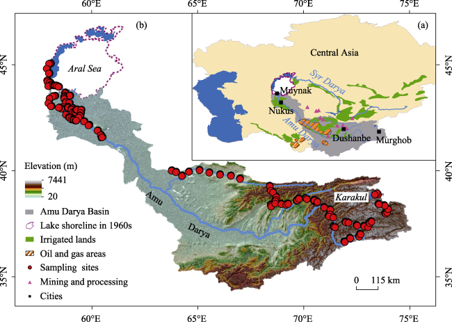
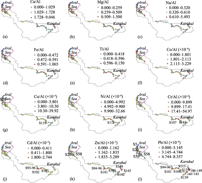
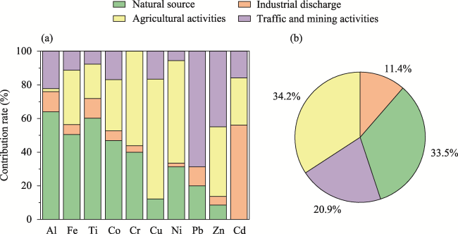
Central Asia (CA) is one of the most fragile regions worldwide owing to arid climate and accumulated human activities, and is a global hotspot due to gradually deteriorating ecological environment. The Amu Darya Basin (ADB), as the most economically and demographically important region in CA, is of particular concern. To determine the concentration, source and pollution status of heavy metals (HMs) in surface sediments of the ADB, 154 samples were collected and analyzed for metals across the basin. Correlation and cluster analysis, and positive matrix factorization model were implemented to understand metals’ association and apportion their possible sources. Cumulative frequency distribution and normalization methods were used to determine the geochemical baseline values (GBVs). Then, various pollution indices and ecological risk index were employed to characterize and evaluate the pollution levels and associated risks based on the GBVs. Results indicated that the mean concentrations of HMs showed the following descending order in the surface sediments of ADB: Zn > Cr > Ni > Cu > Pb > Co > Cd. The spatial distribution maps showed that Cr, Ni, and Cu had relatively high enrichment in the irrigated agricultural area; high abundances of Zn, Pb, and Cd were mainly found in the urban areas. Four source factors were identified for these metals, namely natural sources, industrial discharge, agricultural activities, and mixed source of traffic and mining activities, accounting for 33.5%, 11.4%, 34.2%, and 20.9% of the total contribution, respectively. The GBVs of Cd, Zn, Pb, Cu, Ni, Cr, and Co in the ADB were 0.27, 58.9, 14.6, 20.3, 25.8, 53.4, and 9.80 mg/kg, respectively, which were similar to the regional background values obtained from lake sediments in the bottom. In general, the assessment results revealed that surface sediments of the ADB were moderately polluted and low ecological risk by HMs.

Cite this article

ZHAN Shuie , WU Jinglu , JIN Miao , ZHANG Hongliang . Baseline determination, pollution source and ecological risk of heavy metals in surface sediments of the Amu Darya Basin, Central Asia[J]. Journal of Geographical Sciences, 2022 , 32(11) : 2349 -2364 . DOI: 10.1007/s11442-022-2051-0

1 Introduction

Central Asia (CA), located in the hinterland of Eurasian continent, is of geopolitical and strategic importance. CA countries usually consists of five former Soviet Union countries, with a population of over 75 million by 2020 (The World Bank, 2021). Large part of CA has a semi-arid to arid climate, characterized by scarce precipitation and high evaporation, which is one of the most fragile ecosystems in the world (Jiang et al., 2019; Zhang et al., 2019). Despite the abundance of mineral resources to meet energy needs, irrigated agriculture remains the main economic backbone of most CA countries (Hamidov et al., 2016). Water resources are therefore a critical factor limiting economic development in CA (Mueller et al., 2014; Shen et al., 2021; Zhan et al., 2022). However, the environmental problems in water and sediments caused by the population growth, industrial and agricultural activity strengthened in this region in recent decades are becoming increasingly prominent (Awan et al., 2011; Karthe et al., 2015; Hu et al., 2018).
As the most important river in CA, the environmental aspects of the Amu Darya have always been the focus of research (Ataniyazova, 2003; Crosa et al., 2006; Ma et al., 2020; Zhan et al., 2022). The Amu Darya Basin (ADB), covering several countries, including most of Tajikistan, Afghanistan, and Uzbekistan as well as small of Turkmenistan and Kyrgyzstan, supplies most of their water and other energy resources (Babow and Meisen, 2012). However, under the combined effects of arid climate and aggravated human activities caused by large-scale development of irrigated agriculture and mismanagement of resources, the ecological environment of the ADB has gradually deteriorated and triggered ecological crises (Micklin, 2007; Sun et al., 2019). Most worryingly, high levels of heavy metals (HMs), organic pollutants and other toxic substances were detected in the blood of pregnant women and children in the lower ADB, and a series of health problems such as high infant mortality, low birth weight, growth retardation, acute respiratory diseases, diarrheal diseases and other diseases were observed in the area (Ataniyazova et al., 2001; Kaneko et al., 2003). To date, however, the concentration status and sources of pollutants in the environment throughout the ADB are not clear, which creates great uncertainty for local pollution control and prevention.
Exploring the properties of HMs in sediments can provide clues of anthropogenic effects and identify pollutant source (Kodirov et al., 2018; Liao et al., 2019; Ramazanova et al., 2021; Xiao et al., 2021). Through the analysis of HMs in sediments, Zhang et al. (2021) concluded that in addition to human activities, natural sources of HMs in the Yarlung Tsangpo River basin cannot be ignored; Yang et al. (2021) found that HM concentrations in sediments of karstic environments in Guangxi were primarily influenced by the natural geological background. Lepeltier (1969) have determined the geological baselines by cumulative frequency distribution (CDF) to distinguish the natural sources of HMs from other possible sources in the environmental media. Some studies also conducted HM pollution assessment by establishing regional geochemical baseline values (GBVs) to reveal the origins of pollution and the impact of human activities (Jiang et al., 2021; Magesh et al., 2021). In this study, we determined GBVs for HMs in surface sediments from the entire ADB via a combination of CDF method by normalization method. The present study aims (1) to analyze the concentrations and spatial variation characteristics of HMs in the surface sediments; (2) to quantitatively identify the potential sources of HMs; (3) to assess the pollution levels and potential ecological risk of HMs in surface sediments based on the establishing regional GBVs. Therefore, this study was designed to provide an insight into the levels and sources of the HM pollution in surface sediments from the ADB, which could serve as a reference for subsequent studies.

2 Materials and methods

2.1 Study area

The ADB, located between 34°30′N-43°45′N and 58°15′E-75°07′E, is an essential region for the construction of the Belt and Road (Figure 1). It covers a drainage area of 465,000 km2, of which approximately 200,000 km2 are in the highest mountainous areas of the Pamir Mountains (Wang et al., 2016). The basin is critical to the economy and livelihoods of most of the CA population, housing more than 50 million people (Babow and Meisen, 2012; Salehie et al., 2021). The climate changes drastically according to elevation in ADB, and most of the basin is continental, with dry and hot summer and bitterly cold winter. Average annual precipitation is over 1000 mm in the high mountain areas. However, in the plain areas of the lower ADB, the average annual precipitation is only 100 mm, and evaporation is up to 1150 mm (Awan et al., 2011; Sun et al., 2019). Due to the diversity of geography and the uneven distribution of resources, production activities differ greatly among the countries within the watershed. Countries located in plain areas are rich in arable land resources, and irrigated agriculture occupies an important role. Uzbekistan, for example, has 10.7 million ha of cultivated land and is highly developed in irrigated agriculture (Brody et al., 2020). Whereas, for mountainous countries, cultivated land is very scarce, but rich in water and mineral resources. Consequently, although agriculture remained the main source of economy, the contribution of the mining industry could not be ignored, as in Tajikistan, where it accounted for 30% of the country’s economy (Central Asian Geoportal). In recent decades, with the exploitation of the mineral resources and the development of industry and agriculture, the pollutants released into the environment have increased, which has aroused wide public concern (Skipperud et al., 2013; Shukurov et al., 2014).
Figure 1 Location of the study area and sample sites (a. Geographical location of the Amu Darya Basin (ADB) (based on maps from: www.cawater-info.net/infographic/index_e.htm); b. sampling locations along the ADB)

2.2 Sample collection and laboratory analyses

A total of 154 surface sediment (0-5 cm) samples were collected from the ADB. Sampling in the upper watershed in Tajikistan (samples S88-S154) was completed in October 2011 and in the middle and lower watershed within Uzbekistan (samples S1-S87) in August 2019. Due to the wide extent and topographic complexity of the study area, sample collection was primarily based on accessibility and ensuring the representation of different types of surface sediments. So, some samples in high mountainous areas were collected in the city of Dushanbe as well as along roads. The locations of the sampling sites were determined using a portable GPS (Table S1). Each sample was placed in a clean polyethylene bag and marked with the sample information on the bag. Samples were transported to the laboratory and immediately dried at -50 ℃ for 48 hours using a vacuum freeze dryer (Xiao et al., 2021). The dried samples were then ground using an agate mortar and pestle, and then filtered through a 200-mesh sieve to obtain a powdered precipitate for each sample (Zhan et al., 2020).
Table S1 Geographical information and sample type of each sampling site from the Amu Darya Basin
Sample number Latitude (°N) Longitude (°E) Altitude (m) Sample type
S1 45.09355 58.33991 49 Lake sediment
S2 45.09355 58.33991 49 Lake sediment
S3 45.09355 58.33991 49 Lake sediment
S4 45.09355 58.33991 49 Lake sediment
S5 45.09355 58.33991 49 Lake sediment
S6 45.08100 58.28500 169 Surface soil
S7 44.84970 58.17594 237 Surface soil
S8 44.63425 58.27724 253 Lake sediment
S9 44.30711 58.19944 199 Lake sediment
S10 44.24873 58.21168 200 Lake sediment
S11 44.20356 58.32296 205 Lake sediment
S12 44.12123 58.37802 177 Lake sediment
S13 44.08447 58.38217 52 Lake sediment
S14 44.03806 58.25035 159 Lake sediment
S15 44.06938 58.48456 42 Lake sediment
S16 44.06334 58.52986 42 Lake sediment
S17 44.06374 58.57458 44 Lake sediment
S18 44.05268 58.63508 44 Lake sediment
S19 44.00553 58.72006 43 Surface soil
S20 43.58602 58.54149 61 Surface soil
S21 43.58602 58.54149 61 Surface soil
S22 43.56616 58.47087 139 Surface soil
S23 43.46829 58.31275 121 Lake sediment
S24 43.24963 58.25420 124 Surface soil
S25 43.10358 58.37633 106 Surface soil
S26 43.74127 59.01847 53 Surface soil
S27 43.69632 59.04511 55 Surface soil
S28 43.60181 59.02691 57 Surface soil
S29 43.57479 59.08906 56 Surface soil
S30 43.57326 59.09240 52 Lake sediment
S31 43.57643 59.19847 55 Surface soil
S32 43.59143 59.24620 53 Surface soil
S33 43.59311 59.24783 55 River sediment
S34 43.54094 58.98140 57 Surface soil
S35 43.49767 58.98558 54 Surface soil
S36 43.44212 58.99502 57 Surface soil
S37 43.32688 59.05892 58 Surface soil
S38 43.25219 59.05441 62 Surface soil
S39 43.08343 58.94251 70 Surface soil
S40 43.02525 58.85735 71 Surface soil
S41 42.99213 58.85060 64 Surface soil
S42 43.03840 58.76303 60 Surface soil
S43 43.03928 58.73996 60 River sediment
S44 43.26153 59.22283 63 Surface soil
S45 43.10220 59.16231 59 River sediment
S46 43.06950 59.18316 63 River sediment
S47 43.04217 59.18326 64 Surface soil
S48 43.01655 59.32836 66 Surface soil
S49 43.01680 59.37185 64 Surface soil
S50 42.96537 59.33280 68 Surface soil
S51 42.95107 59.33272 67 Surface soil
S52 42.84504 59.39550 68 Surface soil
S53 42.83670 59.46350 63 Surface soil
S54 42.82429 59.52205 59 Surface soil
S55 42.94456 59.53710 65 Surface soil
S56 42.94863 59.55301 65 Surface soil
S57 42.94097 59.58916 66 Surface soil
S58 42.93484 59.76965 67 Surface soil
S59 42.79991 59.74224 66 Surface soil
S60 42.69659 59.70949 66 Surface soil
S61 42.66465 59.72384 71 Surface soil
S62 42.58851 59.67012 74 Surface soil
S63 42.72045 59.06932 78 Surface soil
S64 42.59878 59.20219 78 Surface soil
S65 42.58216 59.22119 76 Surface soil
S66 42.56713 59.23772 73 Surface soil
S67 42.49287 59.32398 71 Surface soil
S68 42.47515 59.40865 70 Surface soil
S69 42.46643 59.44533 85 Surface soil
S70 42.43592 59.51649 74 Surface soil
S71 42.44735 59.54669 97 River sediment
S72 42.39873 59.90740 110 Surface soil
S73 42.23267 60.13382 85 Surface soil
S74 42.22255 60.11564 85 River sediment
S75 41.97627 60.53220 93 River sediment
S76 41.76745 60.68371 95 Surface soil
S77 41.65196 60.71657 97 River sediment
S78 41.66534 60.74508 100 Surface soil
S79 40.11962 63.97115 201 Surface soil
S80 40.04567 64.17455 213 Surface soil
S81 39.86995 64.45389 228 Surface soil
S82 40.06103 64.77391 262 River sediment
S83 40.13744 65.27059 335 Surface soil
S84 40.02243 65.72429 397 Surface soil
S85 39.92582 66.22062 465 Surface soil
S86 39.87993 66.72873 568 Surface soil
S87 39.72966 67.15202 711 Surface soil
S88 39.39691 68.53305 1332 River sediment
S89 39.18839 68.57274 1586 River sediment
S90 39.11066 68.67744 2572 Surface soil
S91 38.89101 68.83035 1378 River sediment
S92 38.89101 68.83035 1378 Surface soil
S93 38.77032 68.81921 1044 Surface soil
S94 38.77032 68.81921 1044 Surface soil
S95 38.70201 68.79015 952 Surface soil
S96 38.70201 68.79015 952 Surface soil
S97 38.48420 68.59253 751 Surface soil
S98 38.45854 68.59920 716 Surface soil
S99 38.52061 68.58112 794 Surface soil
S100 38.45859 68.59810 701 Surface soil
S101 38.59525 68.77708 840 Surface soil
S102 38.56662 69.06243 846 Surface soil
S103 38.53153 69.28673 1161 Surface soil
S104 38.57540 69.38149 1302 Surface soil
S105 38.71744 69.78759 1178 Surface soil
S106 38.73679 69.80900 1112 Surface soil
S107 38.74585 69.83037 1059 River sediment
S108 38.73182 69.80268 1143 Surface soil
S109 38.80913 69.88612 1171 Surface soil
S110 38.83589 70.20234 1410 Surface soil
S111 38.79659 70.25208 1467 Surface soil
S112 38.72504 70.58348 1683 Surface soil
S113 38.73729 70.60451 1714 Surface soil
S114 38.73729 70.60451 1714 River sediment
S115 38.62752 70.71804 3211 Surface soil
S116 38.62752 70.71804 3211 River sediment
S117 38.67146 70.73767 2492 Surface soil
S118 38.39984 71.05661 1296 Surface soil
S119 38.40920 71.04856 1400 Surface soil
S120 38.30281 71.33420 1595 Surface soil
S121 38.30281 71.33420 1595 River sediment
S122 38.30281 71.33420 1595 River sediment
S123 38.30281 71.33420 1595 River sediment
S124 38.09869 71.31853 1685 River sediment
S125 38.00033 71.27981 1767 Surface soil
S126 37.94815 71.47269 1971 Surface soil
S127 37.51365 71.50823 2065 River sediment
S128 37.51365 71.50823 2065 River sediment
S129 37.48807 71.55858 2134 Surface soil
S130 37.72320 72.05538 2789 Surface soil
S131 37.70797 72.17426 2955 River sediment
S132 36.80858 72.01372 2756 River sediment
S133 36.96022 72.26612 2754 Surface soil
S134 36.98221 72.26279 3187 Surface soil
S135 37.05308 72.67817 2838 Surface soil
S136 37.16689 72.74179 3564 Surface soil
S137 37.57508 72.58197 3534 Surface soil
S138 37.53759 72.91408 4083 Surface soil
S139 37.50136 73.09118 4196 Lake sediment
S140 37.67910 73.16800 3855 Lake sediment
S141 37.67910 73.16800 3855 Lake sediment
S142 37.74847 73.25281 3790 River sediment
S143 38.12428 73.90579 3615 River sediment
S144 38.17011 73.97319 3614 Surface soil
S145 38.17011 73.97319 3614 Lake sediment
S146 38.33600 74.01207 3828 Surface soil
S147 38.49204 73.86530 3915 River sediment
S148 38.49204 73.86530 3915 River sediment
S149 38.56057 73.59594 4656 Surface soil
S150 39.01036 73.55920 3990 Surface soil
S151 39.01339 73.55450 3960 Lake sediment
S152 39.01339 73.55450 3960 Lake sediment
S153 39.01339 73.55450 3960 Lake sediment
S154 39.01081 73.55524 3955 Lake sediment
Inductively coupled plasma mass spectrometry (ICP-MS, Agilent Technologies 7700, USA) was used to measure the concentrations of the metals. The detection limits for these metals were Ca (5 mg/kg), Mg (2 mg/kg), Na (20 mg/kg), Al (20 mg/kg), Ti (1 mg/kg), Fe (5 mg/kg), Zn (2 mg/kg), Pb (0.02 mg /kg), Ni (0.05 mg/kg), Cr (0.1 mg/kg), Cu (0.02 mg/kg), Cd (0.01 mg/kg) and Co (0.01 mg/kg). Reagent blanks were performed alongside sample analyses to ensure the analytical quality. All the values for tested blanks were below 5% of the sample values. Recoveries between the measured values and standard solution were in the range of 91.6%-105.3%. The relative standard deviations (RSD) of the replicates were all within 10%.

2.3 Positive matrix factorization model

Positive matrix factorization model (PMF) is an effective multivariate factor analysis tool for identifying pollution sources (Paatero and Tapper, 1994; Chai et al., 2021). In this study, EPA PMF 5.0 was used to quantify the various sources of metals in surface sediment samples. The model is a decomposition of the original matrix x into three matrices: the factor scores matrix (g), the factor loading matrix (f) and the residual matrix (e). The equation was as follows:
${{x}_{ij}}=\sum\nolimits_{k=1}^{p}{{{g}_{ik}}{{f}_{kj}}+{{e}_{ij}}}$
where xij represents the concentration of HM j in the ith sample; gik represents the source contribution of k in the ith sample; fkj represents the amount of HM j from source k; and eij is residual error obtained by minimizing the objective function Q:
$Q=\sum\nolimits_{i=1}^{n}{\sum\nolimits_{j=1}^{m}{{{\left[ \frac{{{x}_{ij}}-\mathop{\sum }_{k=1}^{p}{{g}_{ik}}{{f}_{kj}}}{{{u}_{ij}}} \right]}^{2}}}}~$
Here, uij is the uncertainty of HM j in the ith sample, calculated as follows:
if c ≤ MDL,${{u}_{ij}}=5/6\times MDL$
otherwise,$~{{u}_{ij}}=\sqrt{{{\left( errorfraction\times c \right)}^{2}}+MD{{L}^{2}}}~$
where the errorfraction represents the RSD, C represents the concentration of HM, and MDL represents the method detection limit.

2.4 Establishment of regional geochemical baseline

The regional GBVs for HMs in the ADB was established using cumulative frequency curves and normalization methods. For the cumulative frequency curves method, GBV for each HMs was determined by plotting CFD curves, where the cumulative frequencies were displayed on the X-axis and the metal concentrations or transformed values of concentrations were displayed on the Y-axis (Lepeltier, 1969). Prior to plotting the CFD curves, a Kolmogorov-Smirnov (K-S) test should be carried out to confirm the normality of the elemental distribution (Karim et al., 2015). The CFD inflection was identified under a linear regression model with p < 0.05 and R2 > 0.9, and the outliers were excluded until the remaining values met this criterion (Wei and Wen, 2012). The inflection point split the graph into a front part (low concentrations) and a back part (high concentrations) (Figure S1); the front part was supposed to have a geological source, while the back part was considered to have anthropogenic sources, or other biological sources (Jiang et al., 2021). Ultimately, the GBV was obtained by averaging the data from the front part of the inflection point. For the normalization method, the inert element Al was chosen as the normalizer to exclude the effect of grain size (Zeng et al., 2014). A linear regression equation was firstly built between each HM and Al as follows:
$C_{H M}=a C_{A l}+b$
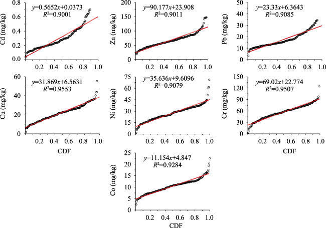
Figure S1 Cumulative frequency distribution (CDF) curves of HMs in surface sediments of the ADB
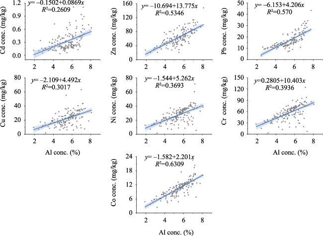
Figure S2 Scatterplot showing the relationship between HMs and Al in surface sediments of the ADB, sample data points do not include the outliers (the sample data points likely affected by anthropogenic activities) shown in Figure 2
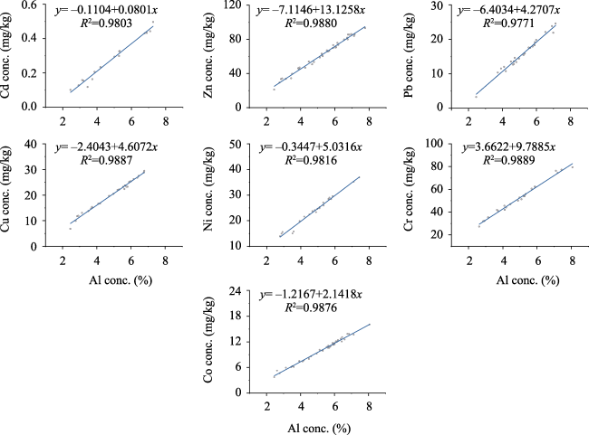
Figure S3 Relationship between HMs and Al, outliers outside 95% confidence band in Figure S2 are further removed and the remaining data points are used to develop GBV
where CHM and CAl represent the concentrations of HM and Al, respectively; a and b are regression constants. In equation (5), natural sediments were determined by points that fell within the 95% confidence interval, while points falling outside the confidence interval were considered to reflect anthropogenic inputs (Zhou et al., 2021). The GBV were therefore calculated by data points that fell within the 95% confidence interval using the following equation:
$GB{{V}_{HM}}=c{{\bar{C}}_{Al}}+d~$
Here, ${{\bar{C}}_{Al}}$ is the mean concentration of Al at selected points; c and d are the redetermined regression constants between HM and Al.

2.5 Pollution assessment

Single-factor pollution index (PI) and pollution load index (PLI) were powerful tools for assessing HM contamination in sediments. Among them, PI reflected the contamination level of an individual HM. The PLI was a combined pollution index calculated from the PI of all HMs. The PI and PLI were defined as follows (Tomlinson et al., 1980):
$P{{I}_{i}}=\frac{{{C}_{i}}}{{{C}_{GB}}}~$
$PLI=\sqrt[n]{P{{I}_{1}}\times P{{I}_{2}}\times P{{I}_{3}}\times \cdots \cdots \times P{{I}_{n}}}~$
where Ci represents the measured HM concentration, and CGB represents the GBV of the HM. Accordingly, HM pollution can be divided into different classifications, shown in Table S2.
Table S2 The corresponding relationship between risk level and value for Eir, RI, PI and PERI
Risk index Risk level Classification level
Eir / PERI Low Eir < 40; PERI < 100
(Magesh et al., 2019) Moderate 40 ≤ Eir < 80; 100 ≤ PERI < 200
Considerable 80 ≤Eir < 160; 200 ≤ PERI <400
High 160 ≤Eir < 320; PERI ≥ 400
Very high Eir ≥ 320
PI / PLI Low PI ≤ 1; PLI ≤ 1
(Jiang et al., 2021) Moderate 1 < PI ≤ 3; 1 < PLI ≤ 2
Considerable 3 < PI ≤ 6
High PI ≥ 6; 2 < PLI ≤ 5
Extremely high PLI > 5
The potential ecological risk index (PERI) was first introduced by Hakanson (Hakanson, 1980). This index is widely used to assess the potential ecological risk of HMs in the sediments. Eir reflected the ecological risk coefficient for individual HM. PERI was the comprehensive ecological risk factor calculated from the Eir of all HMs. The Eir and PERI were defined as follows:
$E_{r}^{i}=T_{r}^{i}\times C_{s}^{i}/C_{n}^{i}$
$\text{ }\!\!~\!\!\text{ }PERI=\sum\nolimits_{n=1}^{n}{E_{r}^{i}}$
Here, Tir represents the toxic-response factor (Zn = 1, Cd = 30, Co = Pb = Cu = 5; Cr = Ni = 2) (Hakanson, 1980); Cis represents the measured HM concentration; Cin represents the reference values of HM. The corresponding classification criteria were also shown in Table S2.

2.6 Statistical analyses

In this study, descriptive statistics were performed using Microsoft Excel 2016. Statistical analyses were conducted on the HMs using SPSS 25.0 software. CFD curves, clustering heat map and cumulative percentage map were plotted using Origin 2018 software. The spatial distributions of normalized metallic elements were mapped using ArcGIS 10.2. EPA PMF 5.0 was applied to analyze and quantify the main sources of elemental metals.

3 Results and discussion

3.1 Concentration variations of metallic elements

Descriptive statistical results of Ca, Mg, Na, Al, Ti, Fe, Cd, Zn, Pb, Cu, Ni, Cr and Co in surface sediment samples from the ADB were listed in Table 1. The concentrations of metals ranged widely and varied significantly between the sampling sites. The coefficients of variation (CV) for most of the metal concentrations exhibited high values except for Al (21.90%), Ti (30.34%), Fe (30.62%) and Co (31.77%), which indicated that the sediments in the ADB probably were affected by discrete inputs associated with anthropogenic activities or natural processes (Adimalla et al., 2020). The highest concentrations of Ca, Mg, Na, Al, Ti, Fe, Cd, Zn, Pb, Cu, Ni, Cr and Co were recorded at sample sites S5, S140, S90, S143, S107, S107, S94, S115, S20, S115, S95, S108, S115, respectively. The lowest concentration of Ca was found at S72, Mg, Ti, Fe, Cu, Ni, Cr and Co at S140, Na at S90, Al at S5, Cd at S141, Pb at S152, Zn at S121. Interestingly, the maximum concentrations of most metallic elements were observed in the mountainous area, primarily located near the city of Dushanbe (such as S90 and S94) and the roadside (such as S108), while the minimum concentrations of most elements were also found in mountainous areas, mainly in remote areas that were less affected by human activities (such as S140, S141 and S152). In addition, the average concentrations of all HMs (Cd, Zn, Pb, Cu, Ni and Cr) exceeded their median values except for Co, suggesting unusually high HM concentrations at some sample sites in the study area.
Table 1 Statistics of elemental concentrations in the surface sediments of the Amu Darya Basin and data on metal concentrations from other study areas
Metals ADB1 (N=154) CSR2 IKLR3 CA4 BMV5
Max Min Ave. Median SD CV (%) Ave. Ave. Ave. Median
Ca (mg/g) 172.2 10.16 68.00 69.44 32.84 48.29 126 15
Mg (mg/g) 46.29 1.87 16.52 16.47 6.20 37.50 10.4 5
Na (mg/g) 175.3 5.24 18.18 14.39 17.24 94.86 5
Al (mg/g) 80.67 19.04 54.46 56.07 11.93 21.90 39 71
Ti (mg/g) 8.65 0.37 2.89 2.96 0.88 30.43 5
Fe (mg/g) 61.45 3.56 27.26 27.77 8.34 30.62 20 31.86 40
Cd (mg/kg) 1.81 0.04 0.36 0.27 0.30 82.55 0.1 0.17 0.43 0.35
Zn (mg/kg) 210.4 20.87 68.73 65.03 29.12 42.36 46.0 77.39 67.40 9
Pb (mg/kg) 52.84 3.28 18.61 15.50 8.71 46.83 11.3 23.92 19.84 35
Cu (mg/kg) 142.8 1.81 23.78 22.53 15.76 66.27 19.5 16.37 22.87 30
Ni (mg/kg) 228.2 1.46 28.37 27.30 19.19 67.64 29.8 20.23 24.82 50
Cr (mg/kg) 384.1 2.88 59.67 58.14 34.11 57.17 56.1 45.78 58.97 70
Co (mg/kg) 22.56 2.40 10.40 10.62 3.30 31.77 8.8 9.55 10.52 8

1 Amu Darya Basin; 2 Caspian Sea region (De Mora et al., 2004); 3 Issyk-Kul Lake region (Ma et al., 2018); 4 Central Asia (Wang et al., 2021a); 5 Worldwide (CNEMC, 1990)

Generally, the average/median concentrations of various metals showed the following descending order in the surface sediments of ADB: Ca > Al > Fe > Na > Mg > Ti > Zn > Cr > Ni > Cu > Pb > Co > Cd (Table 1). Among them, the median concentrations of Ca, Mg, Na, Zn and Co exceeded their corresponding background median values of sediments worldwide (BMVs), while the median concentrations of other metals were within their BMVs (CNEMC, 1990). Also, the average concentrations of HMs were compared with previous relevant studies for other regions in CA (Table 1). It was found that the HM concentrations in surface sediments of the ADB were close to those throughout the CA, except for Zn, Cu and Ni (Wang et al., 2021a). Compared to the surface samples from the Caspian Sea region (CSR) and Issyk-Kul Lake region (IKLR), however, the sediments in the ADB had the highest mean concentrations of Cd, Cu and Cr, especially Cd, while the topsoil in IKLR had the highest average concentrations of Pb and Zn, and the surface samples from the CSR had the relatively high abundance of Ni (De Mora et al., 2004; Ma et al., 2018). The concentration levels of HMs in various regions exhibited large regional differences, which probably were influenced by human activities and the geological environment (Karim et al., 2015; Zhou et al., 2021).

3.2 Normalization and spatial distributions of metals

Assessing the spatial distribution of metals in surface sediments can be a good way to determine positions with higher HM contents and provide evidence of anthropogenic impacts (Chen et al., 2019; Wang et al., 2021a; Yang et al., 2021). To reduce the influence of particle size, and better understand geochemical characteristics and anthropogenic inputs of metal elements, the spatial distribution of metal concentrations with normalized values were essential (Zeng et al., 2014; Zhou et al., 2021). In this study, the conservative reference element, Al was selected as the normalizer, because it had the lowest CV among the metals. High normalized values of Ca, Na and Mg were observed in the lakeside areas, including the Aral Sea and Karakul (Figures 2a-2c), suggesting that these metals tended to flocculate or were susceptible to evaporation (Prabakaran et al., 2019). As for Fe, Ti and Co, they were evenly distributed throughout the basin, with relative enrichment in the downstream plain areas as well as in the riparian and lakeshore areas in the mountains (Figures 2d-2f). Generally, Cu, Ni and Cr were similarly distributed, and relatively enriched in irrigated agricultural areas in addition to urban areas, with lower values recorded around Murghob. High normalized values of Cu, Ni and Cr concentrations were found in sample sites S20 and S119, S115 as well as S107 and S115, respectively (Figures 2g-2i). Whereas, high normalized values of Cd were observed at sample sites S93-S96, S102 and S107, which were mainly located near the industrial outfalls and roads in city of Dushanbe (Figure 2j). In addition, high values of Zn and Pb also occurred in Murghob (such as samples S145, S146, S148 and S149) and in Nukus (such as S58) (Figure 2k-l), which were significantly influenced by human activities such as traffic exhaust emissions (Zhan et al., 2020; Ramazanova et al., 2021).
Figure 2 Spatial distribution of normalized metal concentrations in surface sediments of the Amu Darya Basin

3.3 Source apportionment

3.3.1 Correlation and cluster analysis

To understand whether the sources of the metals were consistent, correlation and cluster analysis were carried out on 15 metals in surface sediments of the ADB. As shown in Figure 3, the metals were divided into two groups. Moreover, a negative correlation or weak correlation between the elements in two groups indicates their different sources. Group 1 represented easily migratory elements, containing Ca, Mg and Na, which were characterized by having active chemical behavior and could be released from the silicate lattice at the initial stage of weathering and then taken with the water (Yang et al., 2021; Zhang et al., 2021). High enrichments of Ca, Mg and Na were observed in sediments from the lower ADB and lakeshore areas (Figure 2), which suffered from sparse precipitation and strong evaporation (Awan et al., 2011). Therefore, group 1 was probably related to the migration and flocculation of chemical elements in sediments as well as the strong evaporation caused by the arid climate. Group 2 contained elements that were very stable in the crust (Al, Fe and Ti) and seven HMs (Co, Cr, Ni, Cu, Pb, Zn and Cd). For the group 2 metals, Al, Fe Co and Ti were strongly correlated with each other, with Fe-Co showing the highest correlation (0.94), indicating that these metals might have the similar origins. In addition, Cr had a highly correlation with Ni (0.93), showing that they probably had the same source. There was also a strong positive correlation between Zn and Pb (0.75), which was similar to the results of previous studies (Hossain et al., 2015). Cu showed moderate positive correlations with Cr and Ni and Cd with Pb and Zn, respectively, indicating that Cu was of similar origins to Cr and Ni and Cd to Pb and Zn. Spatially, Cr, Ni, Cu, Pb, Zn and Cd were primarily enriched in urban as well as agricultural areas and might be heavily influenced by human activities, while Al, Ti, Co and Fe were evenly distributed in the study area and were possibly derived from natural sources (Adimalla et al., 2020; Yang et al., 2021).
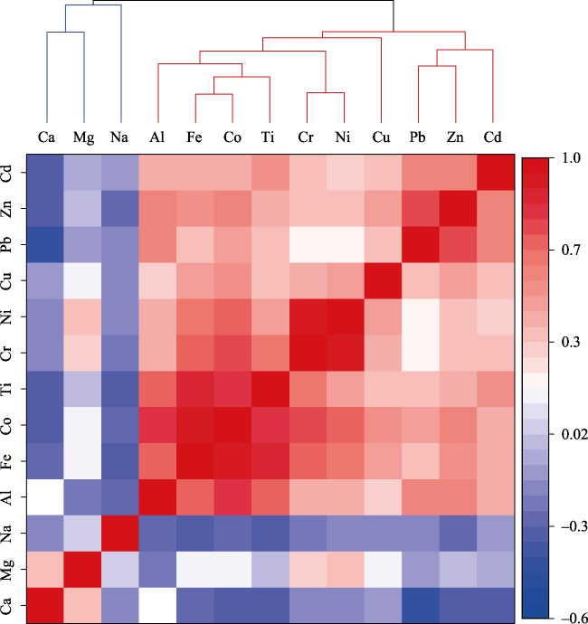
Figure 3 Clustering heat map between metallic elements

3.3.2 Quantitative source by PMF

In order to further assess the anthropogenic and natural sources of metal elements in the sediments, in this study, PMF model was used to quantitatively analyze the sources and contributions of 10 metals in group 2, which were relatively stable in their chemical behavior. The number of factors was set to 3, 4 and 5, respectively, and the model was run 20 times to find the minimum and stable Q value. When the number of factors was 4, the difference between Qrobust and Qtrue was the smallest, and most of the residual were between -3 and 3, and the fitting coefficients R2 between the observed and predicted values of the HMs ranged from 0.85 to 0.99, indicating that the results were reliable (Wang et al., 2020). Four factors were produced by PMF, as presented in Figure 4.
Figure 4 Source composition profiles of metals obtained using the PMF model (a) and percent contribution of each source to the metals in surface sediments of the Amu Darya Basin (b)
The first factor (F1) had higher relative contributions for Al (64.0%), Fe (50.5%), Ti (60.3%) and Co (46.9%) in the sediments of ADB, accounting for 33.5% of the total source contribution (Figure 4). In most environments, Al, Ti, Fe and Co were fairly stable and rarely occurred migration. These metals were probably from the parent rocks, or secondary enrichment during weathering (Taylor, 1964; Yang et al., 2021). In addition, Al, Ti, Fe and Co in our study also exhibited low CVs and more even spatial distribution, indicating that they were less influenced by the environment (Table 1 and Figure 2). Thus, F1 could be considered as a natural source connected to the parent rocks.
The second factor (F2) explained 11.4% of the total variance, which was characterized by Cd (56.1%). The highest CV (85.15%) was observed for Cd among the HMs, indicating that anthropogenic sources were the dominant contribution to Cd contamination. Previous studies had revealed that Cd might come from electroplating industries, fossil fuel combustion and petroleum refining (Gunawardena et al., 2014; Jiang et al., 2021). Spatially, high enrichment of Cd occurred mainly near the industrial sewage outfalls (S94 and S95), roads (S93, S96), and riverbed sediments (S107) in the city of Dushanbe. Therefore, F2 could be identified as a possible source from industrial activities.
The third factor (F3) was predominated by Cr (56.2%), Cu (71.2%), Ni (60.9%) and Zn (41.3%), which accounted for 34.2% of the total contribution. Studies have found that Cu and its compounds were commonly associated with agricultural activities, which were usually added to insecticides and fungicides and found in livestock manure (Luo et al., 2009; Wu et al., 2021). Also, higher concentrations of Cr, Ni and Zn suggested anthropogenic sources such as the use of fertilizers and pesticides (Chen et al., 2019; Xiao et al., 2021). The high accumulation of Cu was exhibited in agricultural areas of the study area, such as samples S20 and S119 (Figure 2). Thus, F3 could be regarded as an agricultural source.
For the fourth factor (F4), Pb (68.7%) and Zn (44.9%) were the main loading elements, accounting for 20.9% of the contribution. It was shown that vehicle exhaust played a major role in Pb enrichment (Chai et al., 2021). Whereas Zn acted as an antioxidant and detergent in lubricants, it was released into the environment as vehicle components wear out (Wang et al., 2020). Their spatial distribution also confirmed that high concentrations of Pb and Zn were mainly observed in urban and roadside areas (Figure 2). In addition, the ADB is rich in metallic mineral resources, and Tajikistan leads the CA region in lead- zinc ore reserves (Central Asian Geoportal; Kodirov et al., 2018). Therefore, F4 could be considered as traffic and mining activities.

3.4 Regional geochemical baseline of the HMs in surface sediments of the ADB

Geochemical baselines can reflect the change of surface environment, and they play a key role in managing environmental pollution (Magesh et al., 2021). Studies showed that the accumulated human activities in the ADB might expose the surface environment to pollution by HMs and other toxic substances (Kodirov et al., 2018; Zhan et al., 2020). Hence, it is crucial to distinguish between geochemical and anthropogenic influences in the ADB by establishing the regional GBVs. The CFD method and normalization method were the most commonly used methods for determining the regional GBVs of various elements in sediments (Lepeltier, 1969; Jiang et al., 2021; Magesh et al., 2021). In this study, both CFD method and normalization method were adopted to calculate the GBVs of the HMs in the study area and the average of the GBV for each HM calculated by the two methods was used as the final determined GBV. The CFD curves and the relationship between Al and HM concentrations were plotted in Figure S1 and Figures S2-S3, respectively. In general, the results of GBVs of HMs calculated by the CDF method were similar with those calculated by the normalized method (Table 2). The average GBVs of Cd, Zn, Pb, Cu, Ni, Cr, and Co in surface sediments of ADB were 0.27, 58.9, 14.6, 20.3, 25.8, 53.4, and 9.80 mg/kg, respectively (Table 2). In addition, the determined GBVs of Cd, Zn, Pb, Cu, Ni, Cr, and Co were also closed to the regional background values obtained from the bottom sediment cores of the Caspian Sea, Issyk-Kul and Sayram Lake, and the standard deviations were 0.04, 15.60, 5.04, 2.65, 1.99, 7.41, and 1.32, respectively. The determined GBVs were then applied to evaluate the pollution status and ecological risk of HMs.
Table 2 Geochemical baseline values established in the Amu Darya Basin and other background values (mg/kg)
HMs M11 M22 Mave3 CS4 LS5 LIK6
Cd 0.22 0.32 0.27 0.19 0.29
Zn 59.63 58.17 58.9 41.6 65.9 79.3
Pb 13.73 15.48 14.6 11.8 15.2 23.7
Cu 19.20 21.39 20.3 14.3 19.5 17.5
Ni 23.83 27.85 25.8 27.4 22.6
Cr 50.02 56.68 53.4 53.0 37.9 44.7
Co 9.61 10.04 9.80 11.5 13.0

1 GBVs of HMs determined by the CDF method; 2 GBVs of HMs determined by the normalization method; 3 average values calculated by the two methods; 4 Caspian Sea (De Mora et al., 2004); 5 Lake Sayram (Zeng et al., 2014); 6 Lake Issyk-Kul (Wang et al., 2021b)

3.5 Pollution assessment of HMs

Pollution indices including PI, PLI, Eir and PERI were employed to evaluate the pollution degree of HMs in surface sediments of the ADB. The evaluation thresholds are defined by the corresponding classification criteria, see Table S2. The results showed the average PI values for the seven HMs in surface sediments of the ADB ranged from 1 to 3, which indicated that the whole study area was generally at a moderate level (Figure 5a). For some sample sites, however, the PI values of selected HMs exceeded 3, revealing a considerably even highly contaminated level. Among them, samples S93, S95, S96, S102, S104, S107, S115 and S119 were recorded as considerably contaminated levels (3 < PI ≤ 6) for Cd, and S94 were recorded as highly contaminated levels (PI > 6) for Cd. Sample S108 and samples S95 and S14 were observed to be considerably contaminated levels for Zn and Pb, respectively. Sample 20 and samples S115 and S119 were exhibited high and considerable contamination levels of Cu, respectively. Besides, sample S115 was also recorded with highly contaminated levels of Cr and Ni. Spatially, Cd, Zn and Pb contamination in sediments mainly occurred near urban factories or along roads, derived from industrial discharges, vehicle exhaust and mining activities (Kodirov et al., 2018; Wang et al., 2020; Chai et al., 2021). For Cu, Ni and Cr, highly contaminated sediments were recorded in agricultural areas, primarily from the extensive use of agricultural fertilizers and pesticides (Luo et al., 2009; Chen et al., 2019; Xiao et al., 2021).The average Eir values for HMs in surface sediments of the ADB were below 40, indicating that the study area was generally at a low ecological risk level, but 3.9% samples of Eir-Cd value were higher than 80 or even 160, which were associated with considerable or high ecological risk level (Figure 5b).
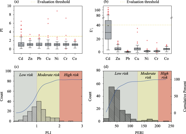
Figure 5 Boxplot of PI (a) and Eri (b) of each HM in different areas, and cumulative percentage of the sum of PLI (c) and PERI (d)
PLI is a simple and comparative index, and is a useful method for examining the combined pollution levels of HMs (Tomlinson et al., 1980; Ramazanova et al., 2021). Similarly, the PLI values also suggested that the surface sediments in ADB were at a moderate pollution level, with 61.7% of the samples having varying degrees of contamination (1 < PLI) (Figure 5c). Of these samples, 2.6% (4 samples) had PLI values between 2-5, which were classified as high risk level, and 59.1% were categorized as moderate risk level (1 ≤ PLI ≤ 2). Overall, 13 samples in the ADB had PERI values in the range of 100-200, indicating a moderate risk level; 1 sample (S94) were recorded as PERI values >200, showing a considered risk level; and the remaining 140 samples exhibited a low risk level (PERI < 100) (Figure 5d).
According to various indices, surface sediments of the ADB were found to be at an overall moderate pollution level of HMs and remained at a low ecological risk level. Relatively severe pollution and high risk were primarily found near urban and irrigated agricultural areas, including the municipality of Dushanbe as well as the farmlands in the lower ADB. This occurrence is in line with the fact that these areas are characterized by intensive human activities such as mining activities, industrial discharges, transport emissions and agricultural fertilizer and pesticide use (Skipperud et al., 2013; Zhan et al., 2020; Ramazanova et al., 2021). Hence, to preserve the ecological environment and economic development, industrial waste and vehicle emissions should be subjected to priority management in urban areas, and the use of fertilizers and pesticides in agricultural areas should be rationalized.
In addition to being influenced by human activities, HMs in surface sediments were also derived from natural sources. Previous studies suggested that high geological background of HMs may be related to their parent rock inheritance or/and secondary enrichment of HMs in the sediments (Yang et al., 2021). Certainly, due to its geographical location, the lower ADB was affected by an arid climate with low precipitation and high evaporation, which also probably contributed to the elevated concentrations of toxic pollutants in water and sediments (Crosa et al., 2006; Awan et al., 2011; Sun et al., 2019). However, our results suggested that HM contamination in surface sediments of the lower ADB was light except for a few sample sites, which indicated that HM pollution might not be the major contributor to human health in the area. Therefore, in our follow-up work, we intend to carry out relevant studies on other pollutants in water and sediments of the watershed that may cause health problems.

4 Conclusion

Correlation and cluster analysis, PMF model, geostatistics and various pollution indices were employed to identify HM sources, establish GBVs and evaluate the contamination levels in surface sediments of the ADB. The mean concentrations of HMs suggested the following descending order: Zn > Cr > Ni > Cu > Pb > Co > Cd. Spatially, the accumulation of HMs was greater in the cities and agricultural area. Four source factors were apportioned by PMF model. Among them, F1 represented the natural sources (Al, Ti, Fe and Co); F2 represented industrial discharge (Cd); F3 was an agricultural source (Cu, Ni and Cr); F4 was a mixed source of traffic and mining activities (Pb and Zn); and F1 to F4 accounted for 33.5%, 11.4%, 34.2% and 20.9% of the total contribution, respectively. GBVs of Cd, Zn, Pb, Cu, Ni, Cr, and Co in surface sediments of ADB were 0.27, 58.9, 14.6, 20.3, 25.8, 53.4, and 9.80 mg/kg, respectively, closing to the regional background values from the Caspian Sea, Issyk-Kul and Sayram Lake. The PI and PLI values indicated that the surface sediments of the ADB were moderately polluted by HMs. Moreover, according to Eir and EPRI results, the ADB remained mostly at a low ecological risk level, with the largest risk being Cd. The research will better understand our cognition of the spatial differences, source, and pollution levels of HMs and design targeted strategies for HMs contamination in the ADB.

We thank the CAS Research Center for Ecology and Environment of Central Asia for assistance with this work, Huawu Wu and Haiao Zeng for field assistances.

[1]
Adimalla N, Chen J, Qian H, 2020. Spatial characteristics of heavy metal contamination and potential human health risk assessment of urban soils: A case study from an urban region of South India. Ecotoxicology and Environmental Safety, 194: 110406.

DOI

[2]
Ataniyazova O A, 2003. Health and ecological consequences of the Aral Sea crisis. The 3rd World Water Forum, Regional Cooperation in Shared Water Resources in Central Asia, Kyoto, Vol. 18.

[3]
Ataniyazova O A, Baumann R A, Liem A K D, et al, 2001. Levels of certain metals, organochlorine pesticides and dioxins in cord blood, maternal blood, human milk and some commonly used nutrients in the surroundings of the Aral Sea (Karakalpakstan, Republic of Uzbekistan). Acta Paediatrica, 90(7): 801-808.

PMID

[4]
Awan U K, Ibrakhimov M, Tischbein B, et al, 2011. Improving irrigation water operation in the lower reaches of the Amu Darya River-current status and suggestions. Irrigation and drainage, 60(5): 600-612.

DOI

[5]
Babow S, Meisen P, 2012. The water-energy nexus in the Amu Darya River Basin: the need for sustainable solutions to a regional problem. Global Energy Network Institute,

[6]
Brody M, Golub A A, Eshchanov B R, 2020. Approaches to optimize Uzbekistan’s investment in irrigation technologies. Ekonomicheskaya politika, 15(2): 136-147.

[7]
Central Asian Geoportal. Mineral resources of the Republic of Tajikistan. http://geoportal-tj.org/index.php/geology/deposits.

[8]
Chai L, Wang Y H, Wang X, et al, 2021. Quantitative source apportionment of heavy metals in cultivated soil and associated model uncertainty. Ecotoxicology and Environmental Safety, 215: 112150.

DOI

[9]
Chen R H, Chen H Y, Song L T, et al, 2019. Characterization and source apportionment of heavy metals in the sediments of Lake Tai (China) and its surrounding sediments. Science of The Total Environment, 694: 133819.

DOI

[10]
China National Environmental Monitoring Centre (CNEMC), 1990. Background Value of Soil Elements in China. Beijing: China Environmental Science Press. (in Chinese)

[11]
Crosa G, Froebrich J, Nikolayenko V, 2006. Spatial and seasonal variations in the water quality of the Amu Darya River (Central Asia). Water Research, 40(11): 2237-2245.

PMID

[12]
de Mora S, Sheikholeslami M R, Wyse E, et al, 2004. An assessment of metal contamination in coastal sediments of the Caspian Sea. Marine Pollution Bulletin, 48(1/2): 61-77.

DOI

[13]
Gunawardena J, Ziyath A M, Egodawatta P, et al, 2014. Mathematical relationships for metal build-up on urban road surfaces based on traffic and land use characteristics. Chemosphere, 99: 267-271.

DOI PMID

[14]
Hakanson L, 1980. An ecological risk index for aquatic pollution control. A sedimentological approach. Water Research, 14(8): 975-1001.

DOI

[15]
Hamidov A, Helming K, Balla D, 2016. Impact of agricultural land use in Central Asia: A review. Agronomy for Sustainable Development, 36(1): 6.

DOI

[16]
Hossain M A, Ali N M, Islam M S, et al, 2015. Spatial distribution and source apportionment of heavy metals in sediments of Gebeng industrial city, Malaysia. Environmental Earth Sciences, 73(1): 115-126.

DOI

[17]
Hu W J, Liu H L, Bao A M, et al, 2018. Influences of environmental changes on water storage variations in Central Asia. Journal of Geographical Sciences, 28(7): 985-1000.

DOI

[18]
Jiang H H, Cai L M, Hu G C, et al, 2021. An integrated exploration on health risk assessment quantification of potentially hazardous elements in sediments from the perspective of sources. Ecotoxicology and Environmental Safety, 208: 111489.

DOI

[19]
Jiang L L, Jiapaer G, Bao A, et al, 2019. Monitoring the long-term desertification process and assessing the relative roles of its drivers in Central Asia. Ecological Indicators, 104: 195-208.

DOI

[20]
Kaneko K, Chiba M, Hashizume M, et al, 2003. Renal tubular dysfunction in children living in the Aral Sea Region. Archives of Disease in Childhood, 88(11): 966-968.

PMID

[21]
Karim Z, Qureshi B A L, Mumtaz M, 2015. Geochemical baseline determination and pollution assessment of heavy metals in urban sediments of Karachi, Pakistan. Ecological Indicators, 48: 358-364.

DOI

[22]
Karthe D, Chalov S, Borchardt D, 2015. Water resources and their management in central Asia in the early twenty first century: status, challenges and future prospects. Environmental Earth Sciences, 73(2): 487-499.

DOI

[23]
Kodirov O, Kersten M, Shukurov N, et al, 2018. Trace metal (loid) mobility in waste deposits and sediments around Chadak mining area, Uzbekistan. Science of The Total Environment, 622: 1658-1667.

[24]
Lepeltier C, 1969. A simplified statistical treatment of geochemical data by graphical representation. Economic Geology, 64(5): 538-550.

DOI

[25]
Liao X Y, Tao H, Gong X G, et al, 2019. Exploring the database of a soil environmental survey using a geo-self-organizing map: A pilot study. Journal of Geographical Sciences, 29(10): 1610-1624.

DOI

[26]
Luo L, Ma Y, Zhang S, et al, 2009. An inventory of trace element inputs to agricultural sediments in China. Journal of Environmental Management, 90(8): 2524-2530.

DOI

[27]
Ma L, Abuduwaili J, Li Y M, et al, 2018. Controlling factors and pollution assessment of potentially toxic elements in topsoils of the Issyk-Kul Lake Region, Central Asia. Soil and Sediment Contamination: An International Journal, 27(2): 147-160.

DOI

[28]
Ma Y, Li Y P, Huang G H, 2020. A bi-level chance-constrained programming method for quantifying the effectiveness of water-trading to water-food-ecology nexus in Amu Darya River basin of Central Asia. Environmental Research, 183: 109229.

DOI

[29]
Magesh N S, Tiwari A, Botsa S M, et al, 2021. Hazardous heavy metals in the pristine lacustrine systems of Antarctica: Insights from PMF model and ERA techniques. Journal of Hazardous Materials, 412: 125263.

DOI

[30]
Micklin P, 2007. The Aral Sea disaster. Annual Review of Earth and Planetary Sciences, 35: 47-72.

DOI

[31]
Mueller L, Suleimenov M, Karimov A, et al, 2014. Novel measurement and assessment tools for monitoring and management of land and water resources in agricultural landscapes of Central Asia. In: Land and Water Resources of Central Asia, Their Utilisation and Ecological Status. Cham: Springer, 3-59.

[32]
Nie M L, Wen Z X, Wang Z M, et al, 2020. Genesis and evaporative fractionation of subsalt condensate in the northeastern margin of the Amu Darya Basin. Journal of Petroleum Science and Engineering, 188: 106674.

DOI

[33]
Paatero P, Tapper U, 1994. Positive matrix factorization: A no-negative factor model with optimal utilization of error estimates of data values. Environmetrics, 5(2): 111-126.

DOI

[34]
Ramazanova E, Lee S H, Lee W, 2021. Stochastic risk assessment of urban soils contaminated by heavy metals in Kazakhstan. Science of The Total Environment, 750: 141535.

DOI

[35]
Salehie O, Ismail T, Shahid S, et al, 2021. Ranking of gridded precipitation datasets by merging compromise programming and global performance index: A case study of the Amu Darya basin. Theoretical and Applied Climatology, 144(3): 985-999.

DOI

[36]
Shen B B, Wu J L, Zhan S E, et al, 2021. Spatial variations and controls on the hydrochemistry of surface waters across the Ili-Balkhash Basin, arid Central Asia. Journal of Hydrology, 600: 126565.

DOI

[37]
Shukurov N, Kodirov O, Peitzsch M, et al, 2014. Coupling geochemical, mineralogical and microbiological approaches to assess the health of contaminated soil around the Almalyk mining and smelter complex, Uzbekistan. Science of The Total Environment, 476: 447-459.

[38]
Skipperud L, Strømman G, Yunusov M, et al, 2013. Environmental impact assessment of radionuclide and metal contamination at the former U sites Taboshar and Digmai, Tajikistan. Journal of Environmental Radioactivity, 123: 50-62.

DOI PMID

[39]
Sun J, Li Y, Suo C, et al, 2019. Impacts of irrigation efficiency on agricultural water-land nexus system management under multiple uncertainties: A case study in Amu Darya River basin, Central Asia. Agricultural Water Management, 216: 76-88.

DOI

[40]
Taylor S R, 1964. Abundance of chemical elements in the continental crust: A new table. Geochimica Et Cosmochimica Acta, 28(8): 1273-1285.

DOI

[41]
The World Bank, 2021. All countries and economies. https://data.worldbank.org/indicator/SP.POP.TOTL.

[42]
Tomlinson D L, Wilson J G, Harris C R, et al, 1980. Problems in the assessment of heavy-metal levels in estuaries and the formation of a pollution index. Helgoländer Meeresuntersuchungen, 33(1-4): 566-575.

DOI

[43]
Wang F F, Guan Q Y, Tian J, et al, 2020. Contamination characteristics, source apportionment, and health risk assessment of heavy metals in agricultural soil in the Hexi Corridor. Catena, 191: 104573.

DOI

[44]
Wang J Z, Wu J L, Zhan S E, et al, 2021a. Spatial enrichment assessment, source identification and health risks of potentially toxic elements in surface sediments, Central Asian countries. Journal of Soils and Sediments, 21(12): 3906-3916.

DOI

[45]
Wang J Z, Wu J L, Zhan S E, et al, 2021b. Records of hydrological change and environmental disasters in sediments from deep Lake Issyk-Kul. Hydrological Processes, 35(4): e14136.

[46]
Wang X L, Luo Y, Sun L, et al, 2016. Attribution of runoff decline in the Amu Darya River in Central Asia during 1951-2007. Journal of Hydrometeorology, 17(5): 1543-1560.

DOI

[47]
Wei C Y, Wen H L, 2012. Geochemical baselines of heavy metals in the sediments of two large freshwater lakes in China: Implications for contamination character and history. Environmental Geochemistry and Health, 34(6): 737-748.

DOI PMID

[48]
Wu M L, Jia Y N, Zhang Y Z, 2021. Heavy metal pollution from copper smelting during the Shang Dynasty at the Laoniupo site in the Bahe River valley, Guanzhong Basin, China. Journal of Geographical Sciences, 31(11): 1675-1693.

DOI

[49]
Xiao H, Shahab A, Xi B D, et al, 2021. Heavy metal pollution, ecological risk, spatial distribution, and source identification in sediments of the Lijiang River, China. Environmental Pollution, 269: 116189.

DOI

[50]
Yang Q, Yang Z F, Filippelli G M, et al, 2021. Distribution and secondary enrichment of heavy metal elements in karstic sediments with high geochemical background in Guangxi, China. Chemical Geology, 567: 120081.

DOI

[51]
Zeng H A, Wu J L, Liu W, 2014. Two-century sedimentary record of heavy metal pollution from Lake Sayram: A deep mountain lake in central Tianshan, China. Quaternary International, 321: 125-131.

DOI

[52]
Zhan S E, Wu J L, Jin M, 2022. Hydrochemical characteristics, trace element sources, and health risk assessment of surface waters in the Amu Darya Basin of Uzbekistan, arid Central Asia. Environmental Science and Pollution Research, 29: 5269-5281.

DOI

[53]
Zhan S E, Wu J L, Wang J Z, et al, 2020. Distribution characteristics, sources identification and risk assessment of n-alkanes and heavy metals in surface sediments, Tajikistan, Central Asia. Science of The Total Environment, 709: 136278.

DOI

[54]
Zhang M, Chen Y N, Shen Y J, et al, 2019. Tracking climate change in Central Asia through temperature and precipitation extremes. Journal of Geographical Sciences, 29(1): 3-28.

DOI

[55]
Zhang W F, Wu J L, Zhan S E, et al, 2021. Environmental geochemical characteristics and the provenance of sediments in the catchment of lower reach of Yarlung Tsangpo River, southeast Tibetan Plateau. Catena, 200: 105150.

DOI

[56]
Zhou Y, Yang X P, Zhang D G, et al, 2021. Sedimentological and geochemical characteristics of sediments and their potential correlations to the processes of desertification along the Keriya River in the Taklamakan Desert, western China. Geomorphology, 375: 107560.

DOI

[57]
Jiang H H, Cai L M, Hu G C, et al, 2021. An integrated exploration on health risk assessment quantification of potentially hazardous elements in sediments from the perspective of sources. Ecotoxicology and Environmental Safety, 208: 111489.

DOI

[58]
Magesh N S, Tiwari A, Botsa S M, et al, 2021. Hazardous heavy metals in the pristine lacustrine systems of Antarctica: Insights from PMF model and ERA techniques. Journal of Hazardous Materials, 412: 125263.

DOI

Outlines

/