Research Articles

Energy dissipation caused by boundary resistance in a typical reach of the lower Yellow River and the implications for riverbed stability

  • XU Haijue , 1, 2 ,
  • LI Yan 1, 2 ,
  • HUANG Zhe , 1, 2, * ,
  • BAI Yuchuan 1, 2 ,
  • ZHANG Jinliang 1, 3
Expand
  • 1. State Key Lab. of Hydraulic Engineering Simulation and Safety, Tianjin University, Tianjin 300072, China
  • 2. Institute for Sediment, River and Coast Engineering, Tianjin University, Tianjin 300072, China
  • 3. Yellow River Engineering Consulting Co., Ltd., Zhengzhou 450003, China
*Huang Zhe (1991-), PhD and Associate Professor, E-mail:

Xu Haijue (1977-), PhD and Associate Professor, specialized in sediment transport and riverbed evolution. E-mail:

Received date: 2021-12-09

  Accepted date: 2022-06-02

  Online published: 2022-11-25

Supported by

National Natural Science Foundation of China(51979185)

National Natural Science Foundation of China(51879182)

National Natural Science Foundation of China(52109097)

Abstract

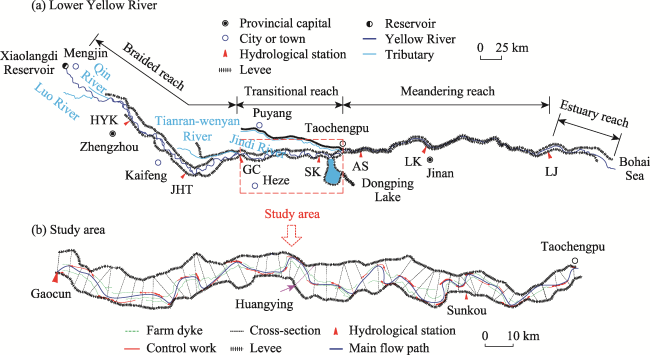
The energy dissipation of boundary resistance is presented in this paper based on the flow resistance. Additionally, the river morphology responses to the resistance energy dissipation are explored using the Gaocun-Taochengpu reach in the lower Yellow River as a prototype. Theoretical analysis, measured data analysis and a one-dimensional hydrodynamic model are synthetically used to calculate the energy dissipation rate and riverbed morphological change. The results show that the energy dissipation rate along the channel will increase in both the mean value and the fluctuation intensity with increasing discharge. However, the energy dissipation rate will first decrease and then increase as the flow section or width-depth ratio increases. In addition, the energy dissipation rate has a significant positive correlation with the riverbed stability index. The results imply that the water and sediment transport efficiency of the river channel can be improved by optimizing the cross-sectional configuration to fulfil the minimum energy dissipation rate of the boundary resistance under stable riverbed conditions.

Cite this article

XU Haijue , LI Yan , HUANG Zhe , BAI Yuchuan , ZHANG Jinliang . Energy dissipation caused by boundary resistance in a typical reach of the lower Yellow River and the implications for riverbed stability[J]. Journal of Geographical Sciences, 2022 , 32(11) : 2311 -2327 . DOI: 10.1007/s11442-022-2049-7

1 Introduction

A natural river can be regarded as a self-adjusting system. The river pattern (wandering, meandering or straight) displayed in spaces and periods is the consequence of the multifaceted adjustment in response to changes in the fluvial environment. The river flow process accompanies the inputs and outputs of energy and material (Leopold and Langbein, 1962) as well as the complex dynamics of energy transfer and conversion. The energy transfer and conversion can lead to changes in the riverbed morphology, hydraulic processes and sediment transport along the channel.
Using energy dissipation theory to investigate water and sediment transport and morphology evolution in river channels has become a topic of high interest. The studies conclude that the energy dissipation trends to the minimum during the adjustment of riverbed morphology (Chang, 1977; Yang, 1979). Leopold and Langbein (1962) first proposed the application of statistical entropy to study riverbed evolution. Then, the concepts of minimum energy dissipation have been applied theoretically to derive the downstream hydraulic geometry exponents of the observed natural river systems (Langbein, 1964; Williams, 1978). Yang (1971; 1979) and Song (1980) systematically proposed the theory of the minimum energy dissipation rate of rivers, and Chang et al. (1977) proposed the theory of minimum stream power. The river energy dissipation rate or stream power both trends to the minimum when the river is in the equilibrium state, which can be used to predict the cross-sectional form of alluvial rivers (Chang, 1979a, 1983, 1984; Yang, 1981, 1991, 1994; Molnár, 1998). After these studies, many scholars have focused on the energy dissipation of rivers, the energy conversion of sediment-laden flow and the responses of the river patterns. Pang (1997) explained the reasons for the energy dissipation in the main channel using the kinetic energy equation of river flow. Physical processes of the momentum exchanges were expressed between the main channel and the floodplain to analyse the redistribution of flow field energy under the influence of the floodplain. Chen et al. (2004) proposed the principle and formula of the minimum energy dissipation rate to maintain the stability of alluvial rivers, based on which a numerical model was established to optimize the water and sediment transport of rivers. Shu et al. (2008) derived the turbulence formula of the kinetic energy conversion rate and efficiency coefficient of sediment suspension based on the energy balance equation of water-sediment two-phase flows. The relationship between the efficiency coefficient and concentration of sediment suspension was obtained in their study. Xu et al. (2016) proposed the energy dissipation rate of rivers based on the analysis of generalized flux and forces. The theory was also applied to study the river pattern and riverbed evolution in the lower Yellow River (Xu, 2013; 2015). Sun et al. (2011) used energy dissipation to systematically analyse the riverbed adjustment in the Inner Mongolia section of the Yellow River. They all found that there was a close correlation between the river morphology and energy dissipation. However, current studies have rarely established a quantitative relationship between energy dissipation and river patterns. Bai et al. (2015) proposed a statistical analysis of the flow resistance induced by river morphology to study sediment movement in rivers. Based on the analysis, the discrimination and activity indicators of river patterns can be expressed by formulas (Xin et al., 2018). Therefore, it is necessary to quantitatively establish the relationship between river energy dissipation and river patterns, as well as riverbed stability.
In this paper, the energy dissipation rate is obtained from the perspective of the boundary resistance of rivers. The Gaocun-Taochengpu (GC-TCP) reach in the lower Yellow River is taken as the research object. Measured data in the field are used to analyse the cross-sectional form variation, thalweg swing and longitudinal gradient changes. A one-dimensional hydrodynamic model is also established based on the topography of river sections for years. Hydraulic factors such as flow width, water depth and slope along the channel are calculated to relate to the variation in the energy dissipation rate of the boundary resistance under various flow conditions. Finally, the stability index of the riverbed is introduced and discussed with the correlation to the energy dissipation rate of the boundary resistance.

2 Study area and data collection

2.1 Study area

The Yellow River is a rare river with plenty of sands in the world with a total length of 5,464 km and drainage area of 795,000 km2. The lower Yellow River (LYR) extends from Mengjin in Henan Province to Lijin in Shandong Province with a length of approximately 785.6 km. The LYR has been divided into three reaches based on morphological features (Wu et al., 2005; Xia et al., 2014), which are the braided reach from Mengjin to Gaocun, the transitional reach from Gaocun to Taochengpu and the meandering reach from Taochengpu to Lijin (Figure 1a). The plan form of the channel gradually narrows from upstream to downstream.
Figure 1 Plan form of the lower Yellow River channel (a) and overview of the study reach (b)
This study focuses on the transitional reach from Gaocun to Taochengpu. The river reach has a famous transitional pattern between braided and meandering morphology, with various cross-section forms and active riverbed evolution (Wu et al., 2005; Xia et al., 2014). This reach has a length of 154 km (see Figure 1b), a longitudinal gradient of 0.118‰ and a bending coefficient of 1.26. Two key hydrological stations named Gaocun (GC) and Sunkou (SK) are located in this river reach. In addition, the Aishan (AS) and Luokou (LK) hydrological stations are located downstream of the reach. Riverine discharge, water level and sediment concentration are routinely monitored at the stations.

2.2 Data collection

In this study, hydrological data, including the water level and discharge during the flood season, are collected at four hydrological stations, Gaocun, Sunkou, Aishan and Luokou. In addition, the cross-section forms in 104 profiles from Gaocun to Luokou are collected in April 2005 and April 2016. The particle size of the bed material (d50) between Gaocun and Taochengpu in 2005 and 2016 is also measured. The above data are all provided by the Yellow River Conservancy Commission of China (YRCC). The data can be used to analyse the impacts of hydrological changes on the geomorphic evolution of the river. Moreover, the data are used in a one-dimensional hydrodynamic model as boundary conditions and for model validation.

3 Method

3.1 Energy dissipation of boundary resistance

The river flow needs to overcome the boundary resistance during the runoff process, resulting in energy dissipation. The process accompanies the constant adjustment of the riverbed to adapt to changes in the fluvial environment and energy conversion and transmission. In the alluvial system, there are different forms of energy dissipation (Knighton, 1984), among which the main component results from the resistance of the boundary to fluid-sediment mixtures (Yang and Song, 1979; Julien, 1995; Molnár, 1998). The boundary resistance has various forms, including bed surface resistance, air surface resistance, and channel morphological resistance (Song and Bai et al., 2015).
The energy dissipation rate can be obtained by integrating the product of the shear stress and the velocity gradient. The energy dissipation rate can be further simplified by neglecting the linear deformation of the riverbed, riverbank or water surface induced by the surface tension of water. The energy dissipation rate can be expressed as follows assuming that the water flow is incompressible and irrotational (Molnár, 1998).
$P=\int_{\forall }{\left[ {{\tau }_{xz}}\left( \frac{\partial {{v}_{z}}}{\partial x}+\frac{\partial {{v}_{x}}}{\partial z} \right)+{{\tau }_{xy}}\left( \frac{\partial {{v}_{x}}}{\partial y}+\frac{\partial {{v}_{y}}}{\partial x} \right)+{{\tau }_{yz}}\left( \frac{\partial {{v}_{z}}}{\partial y}+\frac{\partial {{v}_{y}}}{\partial z} \right) \right]}d\forall $
where P is the total energy dissipation rate in a river reach; τij is the tangential or normal stress;$\forall $is the control volume; and vx, vy, and vz are the flow velocity components (m/s) in the x, y and z directions, respectively. x is the direction of the main flow, y is the direction perpendicular to the main flow, and z is the vertical direction (see Figure 2).
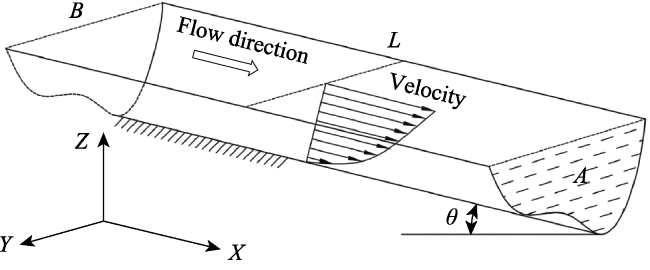
Figure 2 Schematic diagram of coordinates
This study aims to investigate the large-scale behaviour of a river system but the detailed hydraulics in a particular river cross-section. Therefore, a one-dimensional hydrodynamic model is much more applicable. For the one-dimensional flow along the river course (defined with the x direction), the effect of the transverse shear stress caused by the secondary flows is neglected (τzy=0). Considering vy=vz=0, Equation (1) can be simplified to:
$P=\int_{\forall }{\left( {{\tau }_{zx}}\frac{\partial {{v}_{x}}}{\partial z}+{{\tau }_{yx}}\frac{\partial {{v}_{x}}}{\partial y} \right)d\forall }$
where τzx and τyx are the bed shear stress and bank shear stress, respectively, in which the water surface shear stress τw is equal to 0, and the shear stress τzx close to the riverbed is assumed equal to the boundary shear stress τb as a constant.
Considering the wide-shallow shape of the cross-sections in this river, the bank shear stress${{\tau }_{yx}}$can be neglected in Equation (2). Under this assumption, Equation (2) can be reduced to:
$P=L\chi {{\tau }_{b}}\int_{0}^{h}{\frac{\partial {{v}_{x}}}{\partial z}dz}=L\chi {{\tau }_{b}}v(h)$
where L and χ are the channel length and wetted perimeter, respectively; the actual velocity v(h) can be approximated as the depth-averaged velocity u. Then, Equation (3) can be rewritten as:
$P=L\chi {{\tau }_{b}}u$
where u is the depth-averaged velocity that is determined from the discharge and cross-sectional area.
For the uniform flow of the open channel, the shear stress of the riverbed boundary can be written as:
${{\tau }_{b}}\text{=}{{\rho }_{m}}u_{*}^{2}=\frac{1}{8}\lambda {{\rho }_{m}}{{u}^{2}}$
where ρm is the submerged specific density of the fluid-sediment mixture; under the condition of no sediment transport, ρm=ρ; ρ is the density of water. λ is the resistance coefficient, which can be expressed by the Chezy coefficient C with$\lambda =\frac{8g}{{{C}^{2}}}$. Then, Equation (5) is rewritten as:
${{\tau }_{b}}\text{=}{{\rho }_{m}}g{{\left( \frac{u}{C} \right)}^{2}}$
The energy dissipation rate of the boundary resistance per unit length of river reach can then be expressed by:
${{P}_{b}}=\rho \frac{g{{Q}^{2}}}{{{C}^{2}}AR}\cdot \frac{Q}{A}$
where g is the gravity acceleration, Q is the flow discharge, R is the hydraulic radius, and A is the cross-sectional area. Equation (7) shows the energy dissipation rate per unit channel length due to the boundary resistance, in which C=R1/6/n represents the comprehensive roughness coefficient of the channel system.

3.2 One-dimensional hydrodynamic model

The one-dimensional (1-D) hydrodynamic model is applied to simulate the hydraulic parameters of the GC-TCP reach, such as the water depth h, flow width B and flow area A. The governing flow equations include continuity Equation (8) and momentum Equation (9).
$\frac{\partial Q}{\partial x}+\frac{\partial A}{\partial t}=0$
$\frac{\partial Q}{\partial t}+\frac{\partial }{\partial x}\left( \alpha \frac{{{Q}^{2}}}{A} \right)+gA\frac{\partial H}{\partial x}+\frac{gQ\left| Q \right|}{{{C}^{2}}AR}=0$
where H is the water level and α is the momentum correction coefficient.

4 Results

4.1 Validation of the 1-D model

Based on the topography of the cross section in GC-TCP in 2005 and 2016, the mathematical model is established. The flow discharge at GC is set as the inlet boundary condition, and the water level at LK is the outlet boundary condition. The variations in the riverbed roughness coefficient are considered in the model calculation. Figure 3 shows the relationship between the measured roughness coefficient and the flow velocity. The roughness shows no significant changes within the two hydrological stations during 2005- 2017. However, the regular distributions of the roughness with the flow velocity are relatively obvious. Therefore, the various riverbed roughnesses are expressed by Manning’s coefficient with the equation of n=aub. In the equation, a is the coefficient and can be obtained with reference to a=R2/3J1/2, J is the hydraulic gradient, and b is the index. The flow model is solved based on MIKE 11, which is a professional software for hydrodynamics (DHI, 2012). The water levels at the SK and AS in different years are calculated along with the field-measured data for the model validation (shown in Figure 4). The simulation agrees well with the measured data in most regions, and the maximum error is within 0.1 m. Therefore, the 1-D hydrodynamic model is reasonable and can support the subsequent simulation and analysis.
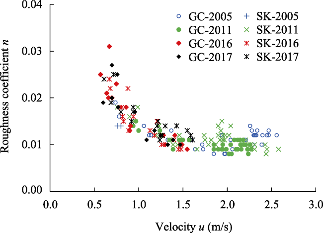
Figure 3 Roughness coefficient distribution at the Gaocun and Sunkou hydrological stations in the lower Yellow River during 2005-2017
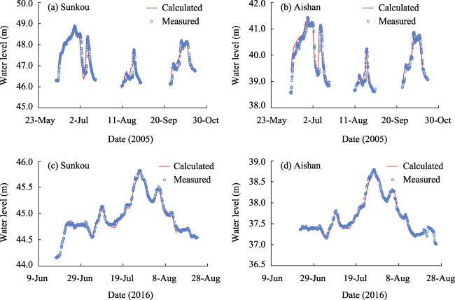
Figure 4 Comparison of the calculated and measured water levels at Sunkou and Aishan stations in the lower Yellow River

4.2 Variations in the riverbed morphology

The variations in the riverbed morphology can be reflected in the cross-sectional form, the longitudinal profile and the plan form (Perucca, 2005). The LYR has typical compound channels with complex cross sections. The main channel is the main route for water and sediment transportation. Therefore, adjustments of the riverbed morphology are focused on in the main channel.

4.2.1 Changes in the longitudinal profile and thalweg migration

After the opening of the Xiaolangdi Reservoir (XLD) in 2000, the riverbed elevation decreased dramatically from 2005 to 2016 along the entire LYR because of the continuous channel incision for a long time. Figure 5a shows the longitudinal changes in the thalweg elevation and the average bed elevation in the GC-TCP. The average riverbed gradient remains at approximately 0.12‰ during 2005-2016, which indicates that the riverbed is equivalently undercut, with an incision depth of 1.50 m. In addition, Figure 5a also shows that the thalweg elevation decreases much more than the average bed elevation in the majority of sections throughout the GC-TCP, with an average incision depth of 2.03 m during the period from 2005-2016. This indicates that scouring at the channel thalweg is more intense, which leads to cross-sectional changes in the GC-TCP.
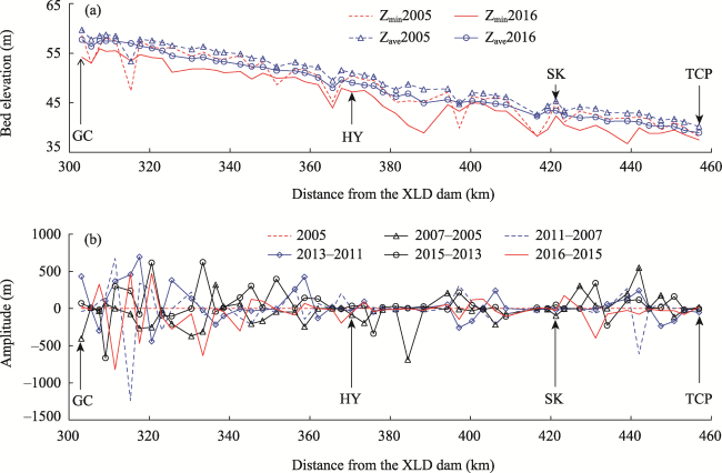
Figure 5 Variations in the riverbed elevation and thalweg migration from the GC to the TCP stations in the lower Yellow River: (a) bed elevation (Zmin is the thalweg elevation of a cross section, and Zave is the average elevation of riverbed); (b) thalweg migration
The horizontal migration of the thalweg is analysed in the GC-TCP during 2005-2016, as shown in Figure 5b (a negative value indicates that the thalweg moves towards the left bank, and a positive value indicates that the thalweg moves towards the right bank). The studied river reach is divided into three subreaches: GC-HY, HY-SK and SK-TCP. The thalweg migration of the GC-HY becomes increasingly larger and has similar characteristics to the channel swinging of the upstream braided reach, with an average migration amplitude of 180 m/a. The maximum migration amplitude can reach 1240 m/a. The thalweg swing of HY-SK is obviously smaller than that of GC-HY. The average migration amplitude can reach 70 m/a, which is similar to the channel swing of the downstream meandering reach. At the SK-TCP, the migration amplitude is approximately 90 m/a. The swing range of the thalweg is largely affected by the incoming flow discharge and sediment flux during the flood season. The flood resulting in greater erosion or sedimentation also leads to the greater swing range of the thalweg. The amplitude of the channel swing has a decreasing trend with the river course downstream, the boundary constraint of the riverbed on the water flow increases, and the riverbed scour resistance is also significantly improved.

4.2.2 Changes in the cross-section form

The adjustments of the cross-section form for the main channel depend on the channel characteristics and the section locations in the LYR. The widening of the cross-section and channel incision widely occur (Li, 2020). Since the operation of the XLD, the riverbed has been continuously coarsened due to sediment erosion and downwards cutting of the LYR due to clear water discharging from upstream. The erosion intensity has then been weakened, and channel widening gradually becomes obvious. The main channel is prone to both downwards incision in depth and sideward erosion in width in relatively straight river reaches, such as the Liyuan (LY), Wushengzhuang (WSZ) and Liangji (LJ) sections. In some sections with relatively large bending degrees, sideward widening is more dominant, such as in the Liuzhuang (LZ), Weitang (WT) and Yingtang (YT) sections (Figure 6).
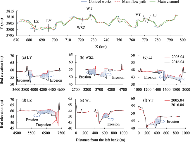
Figure 6 Morphology adjustment of the main channel sections in the lower Yellow River

4.3 Energy dissipation of boundary resistance

Since the operation of the XLD in 2000, the water-sediment regulation scheme has been conducted annually by the YRCC to solve downstream flooding, sediment deposition and other issues (Li and Sheng, 2011). The bank-full discharge increases from 1800 m3/s in 2002 to 4000 m3/s in 2016. Therefore, the bank-full discharge of 4000 m3/s is focused on in detail among the different discharge conditions. The 1-D model is used to calculate the hydraulic parameters, including flow area A, hydraulic radius R, hydraulic gradient J and mean velocity u, for different river topographies under flow discharges of 1000 m3/s, 2000 m3/s, 3000 m3/s and 4000 m3/s. Additionally, the corresponding energy dissipation of the boundary resistance is calculated according to Equation (7). Here, Q = 1000 m3/s is close to the average annual flow rate from 2005 to 2016, while Q = 4000 m3/s can be regarded as the bank-full discharge.
Figure 7 shows the changes in the energy dissipation of the boundary resistance in GC-TCP in 2005 and 2016. The results indicate that the energy dissipation will increase as the flow discharge increases. When the discharge is 1000 m3/s, the resistance energy dissipation rate (Pb) fluctuates with small amplitude from the GC to the TCP with an almost the same average Pb of 1.25 kW/m in 2005 and 2016. When the flow rate increases to 2000 m3/s, the fluctuation of Pb increases with an average Pb of 2.50 kW/m in 2005 and 2.46 kW/m in 2016. When the flow rate further increases to 3000 m3/s and 4000 m3/s, the Pb fluctuation range increases significantly. Under the same discharge, $\overline{{{P}_{b}}}$ is slightly smaller in 2016 than in 2005. However, the difference is not large, which indicates that most cross sections have not changed much in form despite the decrease in the longitudinal gradient of the riverbed with approximately equivalent undercutting or morphological adjustments in a few sections. The morphology of most cross sections in 2016 is generally similar to that in 2005 for GC-TCP.
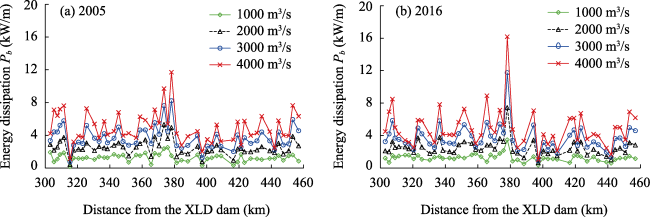
Figure 7 Variations in the energy dissipation rate of the boundary resistance from Gaocun to Taochengpu
The Pb of different sections highly varies along the channel. Some sections have a large Pb exceeding 16 kW/m, such as the Xumatou (XMT) section. However, some sections have a very small Pb of approximately 1.03 kW/m, such as the Xushawa (XSW) section. In this study, the GC-TCP can be divided into two subreaches for detailed discussion according to the changes in Pb (shown in Figure 8). The figure clearly and intuitively shows the mean value and fluctuation intensity of Pb in different river sections. The root mean square ${{\sigma }_{P}}=\sqrt{\overline{{{({{P}_{b}}-\overline{{{P}_{b}}})}^{2}}}}$ is used to express the fluctuating intensity of the resistance energy dissipation rate along the channel, where $\overline{{{P}_{b}}}$ is the average value of Pb. A greater σp means a greater fluctuation of Pb and a farther deflection of the channel from the relative equilibrium state.
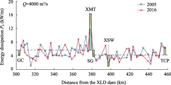
Figure 8 Variations in the energy dissipation rate of the boundary resistance from Gaocun to Taochengpu with a flow rate of 4000 m3/s
According to Table 1, $\overline{{{P}_{b}}}$ and σp are 5.56 kW/m and 2.11, respectively, between the GC and XMT reaches in 2005, while they are 5.51 kW/m and 2.68 in 2016. In the SG (Suge cross-section)-TCP subreach, the two indicators are 4.31 kW/m and 1.39 in 2005, while they are 4.20 kW/m and 1.69 in 2016. The circumstance indicates that the cross-section forms of the downstream subreach do not change much along the channel, and the stability of the river pattern is much better than that of the upstream reach. In addition, Table 1 also shows that Pb has little difference in different years, but the σP of 2016 is higher than that of 2005, which indicates that the intensity of riverbed adjustment in 2016 is higher than that in 2005. Intense adjustment is detrimental to maintaining river channel stability.
Table 1 Average energy dissipation rate and fluctuating intensity in different reaches under a flow rate of 4000 m3/s
Reach 2005 2016
$\overline{{{P}_{b}}}$(kW/m) σP $\overline{{{P}_{b}}}$(kW/m) σP
GC - XMT 5.56 2.11 5.51 2.68
SG - TCP 4.31 1.39 4.20 1.69

5 Discussion

5.1 The energy dissipation rate and the cross-section form

The main channel width and depth are the key factors of the cross-section form of the river. Based on the 1-D hydrodynamic model, the distributions of the flow width and water depth along the GC-TCP are calculated and analysed when the discharge ranges from 1000 to 4000 m3/s. When the discharge increases from 1000 to 4000 m3/s, the average water depth increases from 2.53 m to 4.02 m, which is an increase of 58.88%. The flow width will increase from 397 m to 477 m with an increase rate of 20.18% in 2005. In 2016, the water depth and the flow width also increases at rates of 85.28% and 19.17%, respectively. Notably, the water depth changes are significantly larger than those of the flow width as the flow increased in both years.
The distributions of the flow width B and water depth h under a flow rate of 4000 m3/s are displayed in Figure 9. Both parameters fluctuate along the channel. A mean square root expression is used to quantify the intensity of the fluctuation to better analyse the changes in B and h. The water width and water depth fluctuations along the channel result from the distribution of the energy dissipation of the boundary resistance. A smaller fluctuation intensity indicates that the shape of the river channel section does not change much and that the river channel is approaching a relatively balanced state (Xu et al., 2016). The expression is $\sigma =\sqrt{\overline{{{(X-\overline{X})}^{2}}}}$ (where$\sigma $ represents the intensity of the fluctuation; X is the real value of B or h; and$\overline{X}$is the average value of B or h). According to the formula above, the fluctuation intensities of B and h are calculated in Table 2. According to the table, when the discharge increased from 1000 to 4000 m3/s, the fluctuation intensity of the water depth σh decreases by 28%, while the fluctuation intensity of the water width σB increases by 25% in 2005. However, in 2016, the variation range of σh has a slight response to the flow increase. The fluctuation is reduced, and σh remains at approximately 0.6. However, the increase in σB increases to 57% as the flow rate increases.
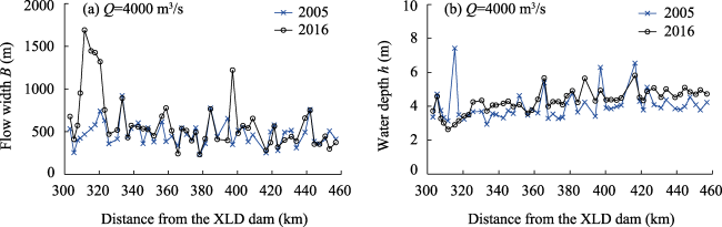
Figure 9 Changes in the flow width and water depth from the GC to TCP reaches for different periods: (a) flow width and (b) water depth
Table 2 Mean flow width, mean water depth and mean fluctuation intensity downstream between the Gaocun and Taochengpu reaches
Discharge
Q (m3/s)
April 2005 April 2016
$\bar{B}$(m) σB $\bar{h}$(m) σh $\bar{B}$(m) σB $\bar{h}$(m) σh
1000 397 111 2.53 1.19 504 202 2.32 0.56
2000 417 129 3.02 1.04 549 248 3.05 0.57
3000 442 134 3.56 0.93 582 294 3.71 0.62
4000 477 139 4.02 0.86 601 317 4.30 0.67
The geometry of the riverbed is the accumulated result of the long-term energy dissipation by boundary resistance. Morphological variables such as the flow area (A) and the width-to-depth ratio (${\sqrt{B}}/{h}\;$) represent the discharge capacity of the river channel and imply the adjustment trend of the cross-sectional form. Figure 10 shows the relationship between Pb and the two variables, with which the trend of the riverbed adjustment can be evaluated. With the operation of the XLD, the channel pattern of this river reach has changed significantly. These changes make it difficult for the flow area to reach 3000 m2 under a discharge of 4000 m3/s. Therefore, some typical cross-sections are collected from the upstream reach adjacent to this river reach for supplementary explanation. The upstream reach has similar flow conditions and riverbed sediment gradation. The details of the supplemented cross sections are shown in Table 3, and the statistical results are shown with grey points in Figure 10. In the figure, Pb first decreases with increasing flow area A or width-to-depth ratio${\sqrt{B}}/{h}\;$ under a bank-full discharge of 4000 m3/s. Then, Pb gradually increases with increasing A or${\sqrt{B}}/{h}\;$. Figure 10a also shows that the energy dissipation rate reaches the minimum at the different flow areas due to different river topographies. In 2005, Pb reached a minimum when the flow area was approximately 2300 m2. In 2016, the corresponding flow area increased to approximately 3200 m2. In addition, Figure 10b shows that under a flow rate of 4000 m3/s, the width-to-depth ratio${\sqrt{B}}/{h}\;$ of the GC-TCP is mostly concentrated in the range of 4–8 in both topographies. Pb tends to be the minimum at width-to-depth ratios of 9 and 10 in 2005 and 2016, respectively.
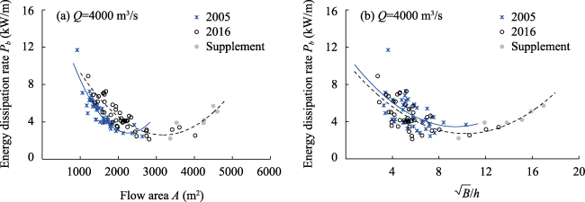
Figure 10 Relationship between the energy dissipation rate of the boundary resistance and flow area A and the width-to-depth ratio${\sqrt{B}}/{h}\;$
Table 3 Supplementary cross-sections from the Huayuankou-Gaocun reach
B (m) h (m) A (m2) ${\sqrt{B}}/{h}\;$ Pb (kW/m) Section (Year)
1020 3.3 3366 9.68 2.21 Babao (2005)
1210 2.92 3533 11.91 3.90 Liubao (2005)
1510 2.81 4243 13.83 3.88 Yuanfang (2016)
1607 2.65 4259 15.13 4.20 Yangxiaozhai (2016)
1750 2.63 4603 15.91 5.10 Sunzhuang (2005)
1800 2.5 4500 16.97 5.71 Xiezhaizha (2016)
The above result shows that the relationship between the energy dissipation rate and the cross-section variables is not a linear change. The adjustment of channel variables typically interact, which makes the relationship between resistance energy dissipation and channel morphology more complicated (Chang, 1977; Yang, 1979). The minimum value of the energy dissipation rate differs for different channel cross-section shapes. When the cross-section shape changes, the resistance energy dissipation will be adjusted accordingly, which in turn affects the changes in the cross-section shape (Zhang et al., 2001). However, after continuous adjustment of the cross-section shape, the energy dissipation rate gradually tends to the minimum value under outside constraints (Chang, 1979b, 1983, 1984; Yang, 1981, 1991, 1994; Molnár, 1998).

5.2 The energy dissipation rate and riverbed stability

Alluvial rivers have an automatic adjustment function. The water flow and sediment transport will be stable within a certain period of time. The river accordingly responds to these processes by adjusting its spatial morphology to maintain a corresponding equilibrium state in the river section width, water depth, riverbed gradient and curvature (Chen, 2004). However, there is no static balance in a natural river but a relatively dynamic balance, as shown in Figure 11a.
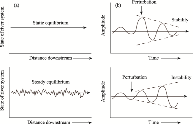
Figure 11 Diagrammatic representation of the types of equilibrium (a); sketches of the definitions of stability and instability in an oscillating mechanical system subject to a perturbation (b) (after Knighton, 1984)
The riverbed of an alluvial river is usually composed of loose sediment particles. During a certain interval, the erosion and deposition changes may have the same intensity for a relatively long river reach. Consequently, the total river reach is in a relative equilibrium state, although the riverbed may be shifted in local subreaches (Ralph and Astrid, 2018). The local riverbed fluctuates around an average value at the relatively balanced state. If the fluctuation amplitude is within a smaller range and gradually decreases with time, the riverbed is in a stable state; if the disturbance amplitude gradually increases with time and exceeds the stability limit, the riverbed is in an unstable state, as shown in Figure 11b.
A smaller fluctuation range means approaching the equilibrium state of the river channel. However, when the river is in a relatively balanced state, the riverbed in local sections may be unstable. The riverbed also has different stabilities for the coming water and sand, as well as for the different cross sections. In this study, the riverbed stability index is used to evaluate the stability of the riverbed in Equation (11) (Wang, 1985). Then, the energy dissipation of the boundary resistance is correlated with the riverbed stability index.
$KK=\frac{{{\tau }_{b}}}{{{\tau }_{B}}+{{\tau }_{c}}}$
where τB is the ultimate bed shear stress of muddy water, which is determined with the suspended sediment concentration and the median size; τc is the critical incipient shear stress of sediment on the clear water bed; and τb is the shear stress on the bed under clear water. In this study, we use the method of Wang (1985) to calculate the ultimate bed shear stress and the critical shear stress.
${{\tau }_{B}}=0.0064{{C}_{m}}+0.098C_{m}^{2}$
${{C}_{m}}=0.788+0.222\lg {{d}_{50}}$
${{\tau }_{c}}={{K}^{*}}\left( {{\gamma }_{s}}-\gamma \right){{d}_{50}}$
where Cm is the sediment concentration on the bed surface (%); d50 is the median bed sediment particle size (mm); K* is the incipient coefficient of sediment and is taken as 0.062 in this paper; γs is the specific weight of a sediment particle; and γ is the specific weight of water.
Table 4 shows the median size of bed sediment in the GC-TCP in the LYR. The riverbed stability index KK for different cross sections can be calculated according to the median particle diameter of the bed material in Table 4. The relationship between KK and Pb is obtained through calculations in 2005 and 2016, as shown in Figure 12. The figure shows that the energy dissipation rate is positively correlated with the riverbed stability index. However, the circumstance does not mean that a larger KK results in more riverbed instability. When the KK is within a certain range, the riverbed is in a stable state without erosion and deposition. When KK is greater or less than the critical range, the riverbed will be unstable. Wang (1985) recommended that when the KK was greater than 0.8 and less than 1, the riverbed remained stable. When KK is greater than 1, the riverbed will be unstable above the upper threshold. When KK is less than 0.8, the riverbed is unstable below the lower threshold.
Table 4 Change in the median particle size between the Gaocun and Taochengpu reaches in the lower Yellow River
Section Distance from the XLD dam (km) Median particle size d50 (mm)
April 2005 April 2016
Gaocun 303.10 0.072 0.131
Susizhuang 330.50 0.111 0.092
Gulou 348.21 0.102 0.128
Yangji 394.31 0.091 0.092
Sunkou 421.30 0.095 0.100
Shilipu 442.00 0.076 0.088
Taochengpu 456.93 0.111 0.102
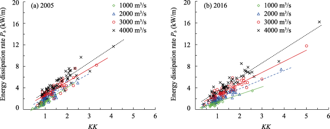
Figure 12 Relationship between the energy dissipation rate of the boundary resistance Pb and riverbed stability index KK
Figure 12 shows that KK is mostly in the range of 0.8~1.0 under a flow rate of 1000 m3/s. Therefore, most riverbeds are in a stable state with a correspondingly smaller energy dissipation rate. The GC-TCP is in a relatively balanced state, as shown in Figure 7. Moreover, at this discharge, the slope in 2016 is slightly flatter, indicating that under the same riverbed stability index, the energy dissipation of the riverbed is smaller in 2016. This circumstance means that the cross sections in 2016 are more effective for water and sediment transport in the river channel. As the flow rate increases, KK also increases. As the flow rate reaches 4000 m3/s, when most of the KK values are greater than 1.0, most sections of the riverbed are above the upper threshold of stability. In addition, there are also some river sections that maintain stability, where the corresponding energy dissipation rate Pb is relatively smaller. However, when the energy dissipation rate tends towards the minimum, the riverbed in some sections may be unstable. For example, some sections still have a KK less than 0.8 below the lower threshold of stability under a flow rate of 1000 m3/s, when the energy dissipation rate tends towards the minimum. In summary, when the energy dissipation tends to the minimum and the KK is in the range of 0.8-1.0, the cross section is more likely to remain stable in this river reach.

6 Conclusions

In this paper, theoretical analysis, mathematical modelling and field-measured data are used to study the relationship between the energy dissipation of boundary resistance and the river morphology in the reach of Gaocun-Taochengpu in the lower Yellow River. The cross-section form and the riverbed stability of the reach are both considered.
Under a constant flow rate, the energy dissipation rate (Pb) fluctuates around the mean value. As the flow rate increases, the mean value and fluctuation intensity of Pb increases, indicating that the river morphology gradually deviates from the relative equilibrium state. Pb first decreases and then increases with changes in the cross-sectional area A and the width-depth ratio ${\sqrt{B}}/{h}\;$ of the river channel. Under the flow rate of 4000 m3/s, when Pb tends towards the minimum, the discharge capacity of the channel in 2016 is significantly higher than that in 2005, which shows that the width-depth ratio is decreasing and the discharge area becomes much larger.
There is a positive linear relationship between the energy dissipation rate Pb and the riverbed stability index KK. When KK is between 0.8 and 1.0, the riverbed section can maintain a stable state. The river regulation plans can be supplemented by using energy dissipation rate analysis combined with the stability index of the riverbed. The cross section can be optimally designed by reducing the Pb towards the minimum under stable riverbed conditions, which can improve the discharge capacity and sediment transport of the river.
[1]
Bai Y C, Wang L Y, Yang S Q, 2015. Discrimination method of bed forms based on the law of resistance. Journal of Hydraulic Engineering, 46(6): 81-87. (in Chinese)

[2]
Chang H H, 1979a. Minimum stream power and river channel patterns. Journal of Hydrology, 41(3/4): 303-327.

DOI

[3]
Chang H H, 1979b. Geometry of river in regime. Journal of the Hydraulics Division, 105(HY6): 691-706.

DOI

[4]
Chang H H, 1983. Energy expenditure in curved open channels. Journal of Hydraulic Engineering, 109(HY7): 1012-1022.

DOI

[5]
Chang H H, 1984. Analysis of river meanders. Journal of the Hydraulic Engineering, 110(HY1): 37-50.

DOI

[6]
Chang H H, Hill J C, 1977. Minimum stream power for rivers and deltas. Journal of the Hydraulics Division, 103(12): 1375-1389.

DOI

[7]
Chatterjee C, Förster S, Bronstert A, 2010. Comparison of hydrodynamic models of different complexities to model floods with emergency storage areas. Hydrological Processes, 22(24): 4695-4709.

DOI

[8]
Chen X J, Hu C H, 2004. Mathematical model for flow and sediment in alluvial river based on minimum rate of available energy dissipation principle. Journal of Hydraulic Engineering, (8): 38-45. (in Chinese)

[9]
Cheng J H, An L H, Wang H, et al, 1997. Analysis of riverbed roughness in the Shandong Reach of the Yellow River. Journal of Hydraulic Engineering, (1): 39-43. (in Chinese)

[10]
DHI, 2012. MIKE11:A modelling system for rivers and channels,Reference Manual, July 2012 Edition. Denmark: Hørsholm.

[11]
Julien P Y, 1995. Erosion and Sedimentation. New York: Cambridge University Press.

[12]
Knighton D, 1984. Fluvial Forms and Processes. Baltimore, USA: Edward Arnold Ltd.

[13]
Langbein W B, 1964. Geometry of river channels. Journal of Hydraulics Division, 90(2): 301-312.

DOI

[14]
Leopold L B, Langbein W B, 1962. The concept of entropy in landscape evolution. U.S. Geol. Surv. Prof. Pap., 500-A, 20pp.

[15]
Leopold L B, Maddock T, 1953. The hydraulic geometry of stream channels and some physiographic implications. U.S. Geol. Surv. Prof. Pap., 252, 57pp.

[16]
Li G Y, Sheng L X, 2011. Model of water-sediment regulation in Yellow River and its effect. Science China Technological Sciences, 54(4): 924-930.

DOI

[17]
Li J, Xia J Q, Ji Q F, 2020. Rapid and long-distance channel incision in the lower Yellow River owing to upstream damming. Catena, 196: 104943.

DOI

[18]
Molnár P, Ramírez J A, 1998. Energy dissipation theories and optimal channel characteristics of river networks. Water Resources Research, 34(7): 1809-1818.

DOI

[19]
Pang B D, 1997. Energy distribution in the flow field of river flood flow. Journal of Hydraulic Engineering, (5): 37-42. (in Chinese)

[20]
Perucca E, Camporeale C, Ridolfi L, 2005. Nonlinear analysis of the geometry of meandering rivers. Geophysical Research Letters, 32(3): L03402.

[21]
Ralph M J S, Astrid B, 2018. A reduced complexity model of a gravel-sand river bifurcation: equilibrium states and their stability. Advances in Water Resources, 121: 9-21.

DOI

[22]
Shu A P, Liu Q Q, Yi Y J, et al, 2008. Characteristics of energy dissipation in hyperconcentrated flows. International Journal of Sediment Research, (4): 107-117.

[23]
Song C C S, Yang C T, 1980. Minimum stream power: theory. Journal of Hydraulics Division, 106(HY9): 1477-1487.

DOI

[24]
Song X L, Bai Y C, 2015. A new empirical river pattern discriminant method based on flow resistance characteristics. Catena, 135: 163-172.

DOI

[25]
Sun D P, Yang Z Z, Zhang L, et al, 2011. Analysis of riverbed form adjustment based on energy dissipation in the Inner Mongolia Reach of Yellow River. Advances in Water Science, (5): 653-661. (in Chinese)

[26]
Wang S Y, Shen H W, 1985. Incipient sediment motion and riprap design. Journal of Hydraulic Engineering, 111(3): 520-538.

DOI

[27]
Williams G P, 1978. Hydraulic geometry of river cross sections: Theory of minimum variance. U.S. Geol. Surv. Prof. Pap., 1029, 47pp.

[28]
Wu B S, Wang G Q, Ma J M, et al, 2005. Case study: river training and its effects on fluvial processes in the lower Yellow River, China. Journal of Hydraulic Engineering, 131 (2): 85-96.

DOI

[29]
Xia J Q, Li X J, Li T, et al, 2014. Response of reach-scale bankfull channel geometry to the altered flow and sediment regime in the lower Yellow River. Geomorphology, 213: 255-265.

DOI

[30]
Xin W Y, Xu H J, Bai Y C, 2018. River pattern discriminant method based on resistance parameter and activity indicators. Geomorphology, 303: 210-228.

DOI

[31]
Xu G B, Yang C T, Zhao L N, 2015. Minimum Energy Dissipation Rate Theory and Its Applications for Water Resources Engineering, Advances in Water Resources Engineering. Springer International Publishing.

[32]
Xu G B, Zhao L N, 2013. Analysis of channel pattern changes in the lower Yellow River based on the rate of energy dissipation. Journal of Hydraulic Engineering, (5): 622-626. (in Chinese)

[33]
Xu G B, Zhao L N, Yang C T, 2016. Derivation and verification of minimum energy dissipation rate principle of fluid based on minimum entropy production rate principle. International Journal of Sediment Research, 31(1): 16-24.

DOI

[34]
Yang C T, 1971. Potential energy and stream morphology. Water Resources Research, 7(2): 311-322.

DOI

[35]
Yang C T, 1994. Variational theories in hydrodynamics and hydraulics. Journal of Hydraulic Engineering, 120(6): 737-756.

DOI

[36]
Yang C T, Kong X B, 1991. Energy dissipation rate and sediment transport. Journal of Hydraulic Research, 29(14): 457-474.

DOI

[37]
Yang C T, Song C C S, 1979. Theory of minimum rate of energy dissipation. American Society of Civil Engineers, 105(7): 769-784.

[38]
Yang C T, Song C C S, Woldenberg M J, 1981. Hydraulic geometry and minimum rate of energy dissipation. Water Resources Research, 17(4): 1014-1018.

DOI

[39]
Zhang O Y, Jin D S, Chen H, et al, 2001. Relationship between energy dissipation rate and channel morphology in the development of the model braided channel. Journal of Geographical Sciences, 11(3): 291-296.

Outlines

/