
Journal of Geographical Sciences >
Dynamic evolution and the mechanism of modern gully agriculture regional function in the Loess Plateau
|
Qu Lulu (1991-), PhD and Lecturer, E-mail: qululu91@cqu.edu.cn |
Received date: 2022-01-26
Accepted date: 2022-09-06
Online published: 2022-11-25
Supported by
National Natural Science Foundation of China(42101202)
National Natural Science Foundation of China(42061037)
National Natural Science Foundation of China and National Science Foundation of the United States Sustainable Regional System Cooperation Research Project(T221101034)
China Postdoctoral Science Foundation Project(2022M710015)
Fundamental Research Funds for the Central Universities(2022CDJSKJC29)
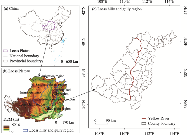
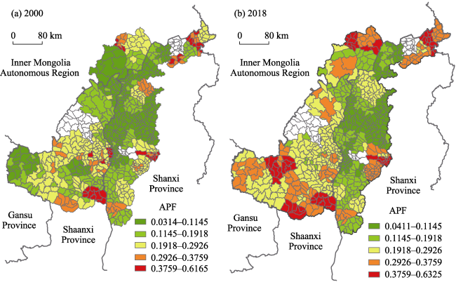
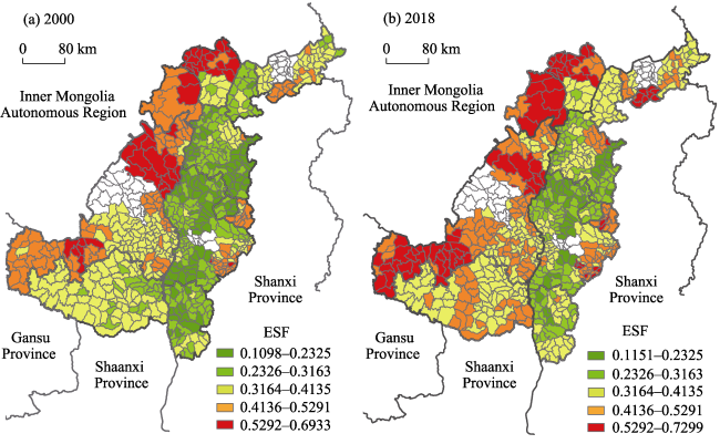
The agricultural regional type and function are the key theoretical issues in agricultural geography research. Gully agriculture in the Loess Plateau is a new regional type of agricultural system with the coupling development of the modern gully human-earth relationship. The study of its functional changes is of great practical significance for food security, rural revitalization and sustainable development of regional agriculture in the region of interest. This paper analyses the multifunctional change of gully agriculture in the Loess Plateau and its dynamic mechanism by using large-scale remote sensing data, topographic relief amplitude model, and spatial econometric model to understand internal implications for evolution differentiation at the basin level. The results show that: (1) The spatial concentration of production and supply function of agricultural products (APF) in the gully of the Loess Plateau gully is high, while the ecological conservation and maintenance function (ECF), employment and social security function (ESF), cultural heritage and leisure function (CRF) are relatively low. The four functions’ spatial distribution has revealed an apparent regularity. (2) APF has been significantly enhanced, which is mainly distributed in point clusters and strips in the farming and pastoral areas in northern Shaanxi to the Yanhe river basin. The high-value areas of ESF are clustered around the urbanized metropolitan circles and urban-rural staggered areas along the Great Wall. ECF is concentrated in areas with significant natural endowments and excellent ecological conditions. CRF is significantly higher in the municipal districts and the surrounding regional central cities. (3) There are noticeable differences in the gully agriculture regional function (GARF) evolution process due to the geographical environment and socio-economic development stages. In this regard, natural factors have tremendously affected APF, ESF, and ECF, while socio-economic factors greatly differ in the four functions. There are still differences in the driving mechanisms of modern gully agriculture evolution types; hence many critical policies in the Loess Plateau can directly affect the function evolution paths. The dynamic evolution of GARF can reflect the general law of rural human-earth system transition in gully areas, thereby providing policy ideas for high-quality development of agriculture in the Loess Plateau.
QU Lulu , LI Yurui , WANG Yongsheng , DONG Shijie , WEN Qi . Dynamic evolution and the mechanism of modern gully agriculture regional function in the Loess Plateau[J]. Journal of Geographical Sciences, 2022 , 32(11) : 2229 -2250 . DOI: 10.1007/s11442-022-2045-y
Figure 1 Geographical location of the study area (Loess Plateau, China) |
Table 1 Evaluation index system of GARF in the Loess Plateau |
| Functional layer | Functional index | Calculation method | Unit |
|---|---|---|---|
| Production and supply function of agricultural products (APF) | D1 Grain yield per unit area | Total grain yield / grain planting area | ton/ha |
| D2 Agricultural output value per unit area | Total agricultural output value / total area of agricultural land, reflecting agricultural production efficiency | ten thousand yuan | |
| D3 Power of agricultural machinery per unit area | It reflects the mechanization level of gully agricultural production | kWh/ha | |
| D4 Per capita non-food cultivation | (Oil + cotton + vegetables + medicinal materials + fruit output) / total population of the region | kg/person | |
| D5 Per capita share of livestock products | (Meat + egg + milk production) / total population of the region | kg/person | |
| Ecological Conservation and maintenance function (ECF) | D6 Total value of ecological services | Ecological service value per unit area of a certain type of land * area of this type of land | ten thousand yuan |
| D7 Amount of chemical fertilizer per unit area | The net amount of agricultural chemical fertilizer / cultivated land area at the end of the year | ton/ha | |
| D8 Pesticide consumption per unit area | Pesticide use / cultivated land area at the end of the year, reflecting the negative impact of pesticides in agricultural production | ton/ha | |
| D9 Forest cover rate | Forest coverage / total area of regional land | % | |
| Cultural heritage and leisure function (CRF) | D10 Leisure agricultural income | Operating income of recreational agriculture such as sightseeing farms and picking gardens | ten thousand yuan |
| D11 Number of agricultural cultural heritage scenic spots | Number of main agricultural cultural heritages in towns | Number | |
| D12 Gully landscape value | A certain type of land area entertainment cultural value * this type of agricultural land area | ten thousand yuan | |
| D13 Urban population above the county level in 100 kilometers around the township | The point distance module tool in ArcGIS, and the calculation and statistics functions of excel such as Vlookup | Person | |
| D14 Annual income per capita in cities above the county level in 100 kilometers around the township | The point distance module tool in ArcGIS, and the calculation and statistics functions of excel such as Vlookup | ten thousand yuan/person | |
| Employment and social security function (ESF) | D15 The proportion of agricultural output value in GDP | Gross agricultural output value / GDP, reflecting the income guarantee of farmers | % |
| D16 Per capita agricultural output value | Gross agricultural output value / agricultural labor force | ten thousand yuan/person | |
| D17 Proportion of agricultural employees | Number of agricultural employees / total rural labor force, reflecting the service level of agricultural employment | % | |
| D18 Rural population | It reflects the carrying level of agricultural population | Person | |
| D19 Farmers’ per capita agricultural income | It reflects the living security level provided by agriculture for farmers | ten thousand yuan |
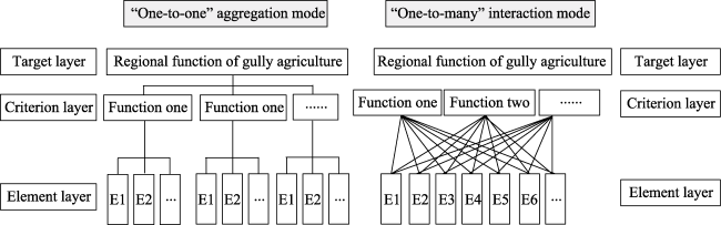
Figure 2 Multi-level correspondence model constructed by the index system |
Table 2 Evaluation index system of GARF in the Loess Plateau |
| Functional layer | Weight | Index layer | Single sort weight value E | Total ranking weight value F |
|---|---|---|---|---|
| D1 | 0.221 | 0.062 | ||
| D2 | 0.213 | 0.059 | ||
| APF | 0.279 | D3 | 0.132 | 0.037 |
| D4 | 0.158 | 0.044 | ||
| D5 | 0.185 | 0.052 | ||
| D6 | 0.251 | 0.066 | ||
| ECF | 0.262 | D7 | 0.234 | 0.061 |
| D8 | 0.132 | 0.035 | ||
| D9 | 0.382 | 0.100 | ||
| D10 | 0.186 | 0.041 | ||
| D11 | 0.272 | 0.060 | ||
| CRF | 0.222 | D12 | 0.267 | 0.059 |
| D13 | 0.133 | 0.030 | ||
| D14 | 0.142 | 0.032 | ||
| D15 | 0.126 | 0.030 | ||
| D16 | 0.086 | 0.020 | ||
| ESF | 0.237 | D17 | 0.158 | 0.037 |
| D18 | 0.225 | 0.053 | ||
| D19 | 0.405 | 0.096 |
Table 3 Four functional values and concentration of gully agriculture in the Loess Plateau in 2000 and 2018 |
| Year | APF | ECF | CRF | ESF | ||||
|---|---|---|---|---|---|---|---|---|
| 2000 | 2018 | 2000 | 2018 | 2000 | 2018 | 2000 | 2018 | |
| Maximum | 0.633 | 0.675 | 0.530 | 0.509 | 0.848 | 0.848 | 0.693 | 0.730 |
| Minimum | 0.040 | 0.037 | 0.003 | 0.006 | 0.017 | 0.013 | 0.110 | 0.115 |
| Average | 0.219 | 0.233 | 0.219 | 0.256 | 0.210 | 0.206 | 0.348 | 0.374 |
| Standard deviation | 0.124 | 0.143 | 0.107 | 0.103 | 0.134 | 0.131 | 0.117 | 0.117 |
| Coefficient of variation | 0.568 | 0.613 | 0.489 | 0.404 | 0.638 | 0.634 | 0.338 | 0.312 |
| Spatial concentration | 0.228 | 0.252 | 0.193 | 0.160 | 0.247 | 0.244 | 0.137 | 0.131 |
Figure 3 Spatial pattern of agricultural product supply function in the Loess Plateau in 2000 and 2018 |
Figure 4 Spatial pattern of employment and social security function in the Loess Plateau in 2000 and 2018 |
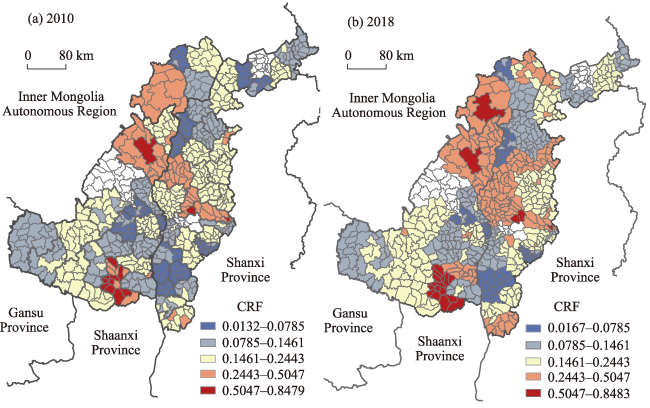
Figure 5 Spatial pattern of cultural heritage and leisure function in the Loess Plateau in 2000 and 2018 |
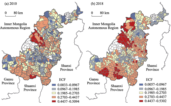
Figure 6 Spatial pattern of ecological conservation and maintenance function in the Loess Plateau in 2000 and 2018 |
Table 4 Influencing factors for regional functional differentiation of gully agriculture in the Loess Plateau |
| Influencing factors | Variable | Influencing factors | Variable |
|---|---|---|---|
| Natural factors | x1 Topographic relief | x9 Proportion of secondary production | |
| x2 Altitude | x10 Per capita fiscal expenditure | ||
| x3 Accumulated temperature | Technological factors | x11 Unit fertilizer consumption | |
| x4 Dryness | x12 Unit mechanical power | ||
| Demographic factors | x5 Population structure | Land benefit factors | x13 Multiple crop index |
| x6 Urbanization rate | Location factors | x14 Geographic conditions | |
| x7 Rural population | Policy factors | x15 Returning farmland to forest index | |
| Socio-economic factors | x8 Per capita household savings | x16 Agricultural capital investment |
Table 5 The calculation results of the four types of GARF evolution influencing factors in the Loess Plateau |
| APF | ECF | ||||||||||
|---|---|---|---|---|---|---|---|---|---|---|---|
| Factors | Variable | MLRM | SEM | SLM | MLRM | SEM | SLM | ||||
| Coefficient | Coefficient | Coefficient | Coefficient | Coefficient | Coefficient | ||||||
| Natural factors | x1 | -0.2036*** | -0.2159*** | -0.1824*** | -0.1259*** | -0.1714*** | -0.1213*** | ||||
| x2 | -0.0455 | -0.0104 | -0.0221 | 0.0138 | 0.0064 | 0.0073 | |||||
| x3 | 0.0793*** | 0.0901*** | 0.0725*** | 0.0292** | -0.0103 | 0.0204 | |||||
| x4 | -0.1016 ** | 0.0223* | -0.0267 | -0.0324 | -0.0191 | -0.0308 | |||||
| Demographic factors | x5 | -0.0082 | -0.0104* | -0.0133 | -0.0075 | -0.0165 | -0.0108 | ||||
| x6 | -0.0767** | -0.0963** | -0.0829** | -0.0220 | -0.0685 | -0.0378 | |||||
| Socio-economic factors | x8 | 0.1212*** | 0.0312** | 0.0638* | -0.0607* | -0.0402 | -0.0565* | ||||
| x9 | -0.0496 | -0.0582** | -0.0606** | -0.0544* | -0.0145 | -0.0458 | |||||
| x10 | 0.0595 | 0.0156* | 0.0403* | 0.0588 | 0.0670** | 0.0599* | |||||
| Technological factors | x11 | 0.1987*** | 0.1666*** | 0.1692*** | 0.0565* | 0.0142 | 0.0443 | ||||
| x12 | -0.1652*** | -0.1512*** | -0.1570*** | -0.0067 | 0.0482 | 0.0064 | |||||
| Land efficiency | x13 | 0.1668*** | 0.1364*** | 0.1464*** | 0.0703* | 0.0207 | 0.0660** | ||||
| Location factors | x14 | 0.0244 | 0.0224** | 0.0144* | 0.0149 | 0.0223 | 0.0077 | ||||
| Policy factors | x15 | 0.1170*** | 0.1546*** | 0.1533*** | -0.0606 | 0.0033 | -0.0392 | ||||
| x16 | 0.1078*** | 0.0266** | 0.0507** | 0.1237*** | 0.1374*** | 0.1227*** | |||||
| C | 0.1540*** | 0.1649*** | 0.0320*** | 0.4542*** | 0.4627*** | 0.3549*** | |||||
| P (Spatial lag) | 0.4207*** | 0.2349*** | 0.3518*** | 0.2027 | |||||||
| λ (Spatial lag) | (0.1015) | (0.1032) | 0.1082 | (0.1089) | |||||||
| Statistical test | R2 | 0.3069 | 0.3917 | 0.3949 | 0.1363 | 0.2226 | 0.1640 | ||||
| Adjustment R2 | 0.2864 | 0.1107 | |||||||||
| F-statistic | 14.9638 | 5.3322 | |||||||||
| LogL | 592.7280 | 629.4719 | 634.7820 | 526.5900 | 555.7679 | 536.9280 | |||||
| AIC | -1143.4600 | -1216.9400 | -1225.5600 | -1011.1800 | -1069.5400 | -1029.8600 | |||||
| SC | -1047.9700 | -1121.4600 | -1125.5300 | -915.6970 | -974.0530 | -929.8280 | |||||
| Spatial dependence test | Moran’s I (error) | 0.6136*** | 0.6582*** | ||||||||
| LMLAG | 36.145*** | 35.0842*** | |||||||||
| R-LMLAG | 1 | 1 | |||||||||
| LMERR | 1 | 1 | |||||||||
| R-LMERR | 1 | 2 | |||||||||
| LAMDA | 0.7382*** | 0.6451*** | |||||||||
| CRF | ESF | ||||||||||
| Factors | Variable | MLRM | MLRM | SEM | SLM | ||||||
| Coefficient | Coefficient | Coefficient | Coefficient | ||||||||
| Natural factors | x1 | 0.2291*** | -0.2502*** | -0.2617*** | -0.2153*** | ||||||
| x2 | 0.0550 | 0.1120 | 0.0119 | 0.0004 | |||||||
| x3 | -0.0810*** | 0.1120*** | 0.0840*** | 0.0967*** | |||||||
| x4 | -0.0332 | -0.0207 | 0.0248 | -0.0049 | |||||||
| Demographic factors | x5 | -0.0205 | 0.0235 | 0.0276 | 0.0219 | ||||||
| x6 | -0.0114 | -0.0072 | -0.0337 | -0.0200 | |||||||
| Socio-economic factors | x8 | -0.0753*** | 0.1561*** | 0.1228*** | 0.1358*** | ||||||
| x9 | -0.0504 | -0.0344 | -0.0213 | -0.0350 | |||||||
| x10 | 0.1428*** | 0.0000 | -0.0328 | -0.0089 | |||||||
| Technological factors | x11 | 0.1349 | 0.1322*** | 0.1066*** | 0.1180*** | ||||||
| x12 | 0.0082 | -0.1389*** | -0.1204*** | -0.1358*** | |||||||
| Land efficiency | x13 | -0.0757*** | 0.0161 | 0.0014 | 0.0165 | ||||||
| Location factors | x14 | 0.1819 | -0.0444** | -0.0273 | -0.0488** | ||||||
| Policy factors | x15 | -0.2119*** | -0.0901*** | -0.0306 | -0.0643** | ||||||
| x16 | 0.2568*** | 0.1870*** | 0.1529*** | 0.1705*** | |||||||
| C | 0.2194 | 0.4115*** | 0.4045*** | 0.3042*** | |||||||
| P (Spatial lag) | 0.5357 | 0.2743*** | |||||||||
| λ (Spatial lag) | (0.0927) | (0.0932) | |||||||||
| Statistical test | R2 | 0.3298 | 0.3403 | 0.3749 | 0.3686 | ||||||
| Adjustment R2 | 0.3100 | 0.3208 | |||||||||
| F-statistic | 16.6316 | 0.0967 | |||||||||
| LogL | 550.8870 | 649.9640 | 663.6799 | 663.9680 | |||||||
| AIC | -1059.7700 | -1257.9300 | -1285.3600 | -1283.9400 | |||||||
| SC | -964.2910 | -1162.4500 | -1189.8800 | -1183.9100 | |||||||
| Spatial dependence test | Moran’s I (error) | 0.4639 | 0.5437*** | ||||||||
| LMLAG | 19.6297 | 39.5286*** | |||||||||
| R-LMLAG | 1 | 1.0359 | |||||||||
| LMERR | 1 | 1 | |||||||||
| R-LMERR | 2 | 2 | |||||||||
| LAMDA | 0.5357 *** | ||||||||||
Note: ***, ** and * represent the significance levels of 0.01, 0.05 and 0.1, respectively. |
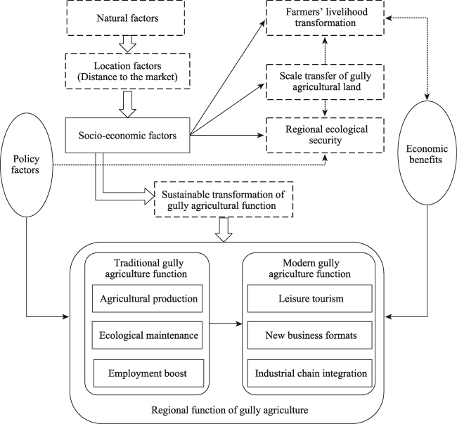
Figure 7 Impact mechanism of GARF in the Loess Plateau |
| [1] |
|
| [2] |
|
| [3] |
|
| [4] |
|
| [5] |
|
| [6] |
|
| [7] |
|
| [8] |
|
| [9] |
|
| [10] |
|
| [11] |
|
| [12] |
|
| [13] |
|
| [14] |
|
| [15] |
|
| [16] |
|
| [17] |
|
| [18] |
|
| [19] |
|
| [20] |
|
| [21] |
|
| [22] |
|
| [23] |
|
| [24] |
|
| [25] |
|
| [26] |
|
| [27] |
|
| [28] |
|
| [29] |
|
| [30] |
|
| [31] |
|
| [32] |
|
| [33] |
|
| [34] |
|
| [35] |
|
| [36] |
|
| [37] |
|
| [38] |
|
/
| 〈 |
|
〉 |