Review Article

Three-dimensional delineation of soil pollutants at contaminated sites: Progress and prospects

  • TAO Huan , 1, 3 ,
  • LIAO Xiaoyong , 1, * ,
  • CAO Hongying 1 ,
  • ZHAO Dan 2 ,
  • HOU Yixuan 1
Expand
  • 1. Institute of Geographic Sciences and Natural Resources Research, CAS, Beijing 100101, China
  • 2. Chinese Academy of Environmental Planning, Beijing 100012, China
  • 3. University of Chinese Academy of Sciences, Beijing 100049, China
* Liao Xiaoyong (1977-), PhD and Professor, specialized in evaluation and remediation of soil pollution. E-mail:

Tao Huan (1989-), PhD, specialized in data mining and analysis of soil pollution. E-mail:

Received date: 2022-04-25

  Accepted date: 2022-06-12

  Online published: 2022-10-25

Supported by

National Natural Science Foundation of China(42130713)

National Key R&D Program of China(2020YFC1807400)

Abstract

The precision remediation and redevelopment of contaminated sites are crucial issues for improving the human settlement and constructing a beautiful China. Three-dimensional delineation of soil pollutants at contaminated sites is a prerequisite for precision remediation and redevelopment. However, a contaminated site is a three-dimensional complex system coupling multiple spatial elements above- and under-ground. The complexity incurs high uncertainties about the three-dimensional delineation of soil pollutants based on sparse borehole and spatial statistics and inference models. This paper first systematically reviewed the objectives of fine three-dimensional delineation of soil pollutants, the sampling strategies for soil boring, the commonly used models for delineating soil pollutants, and the relevant cases of applying these models at contaminated sites. We then summarized the effects of borehole data and three-dimensional models on soil pollutants’ delineation results from biased characteristics and nonstationary conditions. The present research status and related issues on correcting the biased characteristics and nonstationary conditions were analyzed. Finally, based on the problems and challenges, we suggested the three- dimensional delineation of soil pollutants in the underground “black box” for future research from the following six priority areas: multi-scenarios, nonstationary, non-linearity, multi-source data fusion, multiple model coupling, and the delineation of co-contaminated sites.

Cite this article

TAO Huan , LIAO Xiaoyong , CAO Hongying , ZHAO Dan , HOU Yixuan . Three-dimensional delineation of soil pollutants at contaminated sites: Progress and prospects[J]. Journal of Geographical Sciences, 2022 , 32(8) : 1615 -1634 . DOI: 10.1007/s11442-022-2013-6

1 Introduction

A site comprises natural elements (e.g., soil, groundwater, and surface water), human elements (e.g., buildings, structures, and facilities), and living organisms (e.g., microorganisms, earthworms, and vegetation) within a land area. The soil at a site refers to the loose layer of the earth’s land surface composed of minerals, organic matter, water, air, and biological organisms (Li et al., 2009). With the acceleration of China’s urbanization process and the gradual advancement of the industrial restructuring policy of suppressing the second industry and developing the third, industrial enterprises in some cities have been relocated, renovated, or closed consecutively (Liao et al., 2011; Fang et al., 2017). Some industrial enterprises become or are becoming abandoned contaminated land known as legacy industrial contaminated sites due to a lack of strict control during the production. Common legacy industrial contaminated sites included organic-, inorganic- and co-contaminated sites. When these sites are redeveloped and utilized, soil pollution in and around the site causes significant adverse effects on the human settlement (McIntyre et al., 2018). Since the incomplete understanding of pollutants’ characteristics in the underground soil environment during the investigation stage, pollution incidents have frequently been reported in recent years during the redevelopment (Cao et al., 2018). Most incidents are triggered by unscientific remediation actions and insufficient control of secondary pollution during remediation. Therefore, it is urgent to examine the fine three-dimensional delineation of soil pollutant content in the site (site pollution delineation or characterization) before starting costly soil remediation of contaminated sites.
However, limited by the underground “black box” with complex hydrogeological conditions, it is difficult to accurately retrieve the distribution characteristics of soil trace elements using geophysical detection methods (Liao et al., 2018a). Spatial statistics and inference models can estimate the pollutants’ content at unsampled points based on discrete data collected from three-dimensional boreholes. In the estimation process, other multi-source, heterogeneous and spatial auxiliary information can be effectively integrated into the spatial statistics and inference models to obtain reliable results for site pollution delineation (Liu et al., 2017; Liu et al., 2020; Li et al., 2022; Zeng et al., 2022a). In the past few decades, much work has been done on the delineation of soil pollutants in two dimensions based on spatial statistical theory, and some significant progress has been made (Goovaerts, 1999; Xie et al., 2011; Li and Heap, 2014; Liao et al., 2018b). Although some progress has been made in the three-dimensional delineation theory, the delineation results based on discrete soil boring data and spatial statistical inference models still have high uncertainty due to the strong heterogeneity of soil pollutants at contaminated sites (Li et al., 2007; Boudreault et al., 2016). The uncertainty of the site pollution delineation may be propagated to subsequent decision-making based on the site investigation, such as the diagnosis of pollution risks, the delineation of polluted boundaries, and the implementation of remediation project (Troldborg et al., 2012). Firstly, high uncertainty may incur false negatives in diagnosing pollution risks. In addition, high uncertainty may cause over-remediation due to the exaggeration of polluted scopes during the delineation of polluted boundaries. Finally, high uncertainty may lead to secondary pollution due to underestimating the polluted scopes and insufficient remediation. It is challenging to reduce the uncertainty of site pollution delineation and promote the underground “black-box soil” to “transparent soil” due to soil pollutants’ strong spatial variability and soil borehole data’s biased characteristics.
Given the lack of theoretical research on the site pollution delineation application and the refinement of related research results are insufficient, we first systematically reviewed the objectives of site pollution delineation, borehole layout for different objectives of site pollution delineation, commonly used models for site pollution delineation and related cases on applying these models at contaminated sites. We then summarized the effects of soil boring data and three-dimensional models on the soil pollutants’ delineation results from biased characteristics and nonstationary conditions, respectively. The present research status and related issues on correcting biased characteristics and nonstationary conditions were analyzed. Finally, based on the problems and challenges, we suggested the three-dimensional delineation of soil pollutants in the underground “black box” for future research from the following six priority areas: multi-scenarios, nonstationary, non-linearity, multi-source data fusion, multiple model coupling, and the delineation of co-contaminated sites. The present works could provide a promising method for revealing the three-dimensional spatial differentiation of soil pollutant content in the underground “black box” environment.

2 The objectives of site pollution delineation and borehole layout

The purpose of the contaminated sites survey usually includes three aspects: calculating the dosage of remediation chemicals, estimating the polluted volumes, and assessing the stratified health risk. The corresponding site pollution delineations are three-dimensional interpolation for pollutants distribution, delimitation for remediation scopes, and estimation of stratified mean concentration. Interpolation for pollutants’ three-dimensional distribution estimates pollutants’ content at unsampled points in the site based on discrete soil boring data (Li et al., 2007). Delimitation for remediation scopes compares the value of unsampled points with standard thresholds based on discrete soil boring data (Juang et al., 2008). Estimation of stratified mean concentration computes mean concentrations of pollutants within different stratum to assess stratified pollution risks (Volchko et al., 2020).When soil testing and formulated chemical agent is precisely targeted for in-situ remediation at contaminated sites, it is necessary to estimate the pollutants’ content at unsampled points in the three-dimensional space of the site. Then the pollutants’ content at each unsampled point is converted into the prescription map of the remediation chemicals that needs to be injected through the chemical reaction process (Figure 1a). Unlike three-dimensional interpolation for pollutants distribution, the delimitation for remediation scopes only needs to compare the estimated concentration of pollutants in the site and the standard threshold. Pollutant content greater than the standard threshold are areas that need to be remediated. When finely delineating the remediation scopes, the uncertainty of the site pollution delineation inside and outside the boundary is low. High uncertainty is often located in the transition areas which is described by a specific confidence interval from the standard threshold (Figure 1b). These transition areas are often used in the following density sampling (van Meirvenne and Goovaerts, 2001; Gao et al., 2017). The mean stratified concentration of pollutants is an essential input parameter for the risk assessment models to assess stratified health risks, for example, the Risk-Based Corrective Action (RBCA, US), Contaminated Land Exposure Assessment (CLEA, UK), and Health and Environmental Risk Assessment (HERA, China).
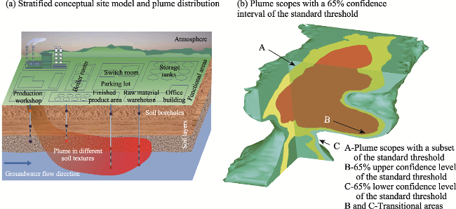
Figure 1 The objectives of three-dimensional delineation of soil pollutants at contaminated sites
The spatial sampling design is to rationally select and allocate sampling sites based on deeply excavating the existing prior knowledge (Jiang et al., 2009). Brus et al. (1997) divide the spatial sampling strategies into design-based and model-based methods. The design-based method believes that the population of values is regarded as unknown but fixed, each sample has a selection probability, and the parameters of the population, such as the mean, are estimated based on the distribution assumption of the sample values. According to the selection probability of the sample, design-based sampling can be further divided into equal probability sampling (random sampling, stratified sampling, and systematic sampling) and unequal probability sampling (judgment sampling). The model-based sampling acknowledges that all sample values obtained are a single realization of a stochastic process inherent in the sample, and the population is infinite. In model-based sampling, the investigator needs to predefine the objective function and then use an optimization algorithm to solve the objective function to obtain the optimal sampling layout. Model-based spatial sampling is suitable for estimating the spatial distribution of pollutant content, such as three-dimensional interpolation for pollutants’ distribution and delimitation for remediation scopes. Commonly used objective functions include semivariograms, even coverage for geographic space and feature space (Chadalavada et al., 2011; Wang et al., 2012).
According to the status of the available prior knowledge before the borehole layout, such as historical soil boring data and auxiliary variable information, the borehole layout at contaminated sites can be classified into four scenarios (Table 1). The historical three- dimensional soil boring data at contaminated sites can directly represent the spatial distribution of soil pollutants, while auxiliary variable information at contaminated sites can potentially characterize the distribution of pollutants. Common auxiliary data include retrieving resistance signals by geophysical detection technology, such as soil temperature field or hydrodynamic field. The distribution of underground pipelines and structures retrieved by ground-penetrating radar is also a vital reference for borehole layout. Additionally, the distribution of above-ground buildings, manufacturing shop design drawings, and historical archives of production management at the investigated site need to be collected (Liao et al., 2018a; Zeng et al., 2022a).
Table 1 The strategies of borehole layout in different scenarios of prior knowledge at contaminated sites
Scenarios of prior knowledge Strategies of borehole layout
Historical soil boring data in geographic space Auxiliary variable information in feature space
No No Systematic or random sampling
No Yes Even sampling in geographic or feature space, judgmental sampling, or purposive sampling
Yes No Densify sampling in geographic space
Yes Yes Densify sampling in geographic space or even sampling in feature space
Scenario 1: Neither historical soil boring samples nor auxiliary data is available. Since the investigators lack the understanding of pollutant information, systematic or random sampling strategies can be adopted.
Scenario 2: There is no historical soil boring data at the contaminated site, but auxiliary data can be collected. The method of even sampling in geographic or feature space based on auxiliary data is the prior choice (Wang et al., 2010; Brus et al., 2019). In addition, judgmental sampling or purposive sampling can also be used. Even sampling of boreholes at contaminated sites includes even coverage for each functional production area horizontally (Zhao et al., 2019), even coverage for each stratified layer vertically (Grauer-Gray and Hartemink, 2018), and even coverage for each quantile interval of pollutant content of concern (Pan et al., 2015) (Figure 1a). In judgmental or purposive sampling, sampling sites are selected based on the investigator’s empirical judgment of the potential pollution distribution at contaminated sites (Liu et al., 2013a; Tao et al., 2017). Judgmental sampling can effectively utilize the historical data and field observation results of contaminated sites, but the statistical inference model may have a high bias in the estimation. The quality of the sample depends on the investigator’s experience and the completeness of the information obtained.
Scenario 3: There are historical soil boring data at contaminated sites but a lack of auxiliary data. Due to the concealment of soil pollution and the constraints of survey costs, multi-stage sampling strategies during contaminated site investigation are commonly employed (Verstraete and Van, 2008; Marchant et al., 2013). When there is historical data, the semivariogram can be fitted by historical soil boring samples first and then densify the samples based on spatial autocorrelation.
Scenario 4: Historical soil boring and auxiliary data are available at contaminated sites. Relevant auxiliary variables can be fused to obtain accurate semivariograms when investigators use the sparse borehole to guide supplementary sampling (Troldborg et al., 2012; Kang et al., 2020). However, high uncertainty of available auxiliary variables is often detected. Based on evaluating the uncertainty of multi-source covariate data (soft data) and analyzing the internal relationship between it and the target variable, some researchers tried to adopt the Bayesian framework to integrate those soft data to improve the fit accuracy of semivariogram (Chen et al., 2012; Li et al., 2022; Zeng et al., 2022a). In addition, auxiliary variables can also be used to design the evenly sampling by optimizing the feature space and then achieve the multi-objective optimization for borehole layout in geographic space and feature space, such as Latin hypercube and variance quadtree methods (Minasny and McBratney, 2006; Minasny et al., 2007).

3 Three-dimensional delineation models at contaminated sites and related cases

Site pollution delineation models of interpolation for pollutants’ distribution can be divided into two categories: non-geostatistical interpolation method (deterministic interpolation) and geostatistical interpolation method (probabilistic interpolation) (Li et al., 2014). The deterministic interpolation method includes inverse distance weighting (IDW), natural neighbor, and Voronoi / Delaunay. The geostatistical interpolation method includes but is not limited to ordinary Kriging, indicator Kriging, co-Kriging, and regression Kriging (Table 2). Compared with the deterministic interpolation method, the geostatistical interpolation method can obtain higher prediction accuracy since it can more genuinely reflect the spatial structure of borehole data and the local heterogeneity of soil pollutants. Furthermore, the geostatistical interpolation method can estimate the uncertainty of the prediction results when the prior knowledge is insufficient, which provides the reliability of the estimated results for decision-makers or risk assessors. Unfortunately, unbiased and optimal interpolation based on geostatistical methods must satisfy the second-order stationary assumption or intrinsic assumption (Matheron, 1963). Due to the complex causes of soil pollution in the underground “black box” environment, the spatial distribution of pollutant content result from the three-dimensional interpolation model based on stationary assumption has a significant deviation from the actual one. The research on the site pollution delineation based on nonstationary is the most promising method for revealing the spatial differentiation of soil pollutants in the underground “black box” environment. However, the application of its theory in contaminated sites needs to be further studied.
Table 2 Summary of case studies on the application of spatial statistics to the management of contaminated sites
Pollution medium Delineation method Software tools1) Pollutant types Function2) Location of case Reference
Soil Ordinary kriging MVS/EVS$ Organic pollutants (3), (6), (7) A chemical plant in Chongqing, China Liu et al., 2017
Soil Ordinary/Indicator kriging MVS/EVS$ Organic pollutants (3), (7) Beijing Coking Plant, China Tao et al., 2014
Soil Moran’s I, LISA Open GeoDaΩ Organic pollutants (5), (6) Beijing Coking Plant, China Liu et al., 2013a
Soil Ordinary kriging MVS/EVS$ Organic pollutants (1) A chemical plant in Hebei, China Tao et al., 2017
Soil Ordinary kriging MVS/EVS$ Organic pollutants (3), (6) A chlorobenzene plant in Jiangsu, China Ren et al., 2016
Soil Kriging, IDW, Nearest neighbor MVS/EVS$ Organic pollutants (3), (6), (7) A leather factory in Shandong, China Men et al., 2017
Soil Ordinary kriging MVS/EVS$ Organic pollutants (4), (7) A chemical plant in Shanghai, China Guo et al., 2009
Soil Ordinary kriging Voxler$ Heavy metals (3) A chemical plant in Shanghai, China Li et al., 2017
Soil Ordinary kriging, Conditional simulations GS+$, ArcGIS$ Heavy metals (4), (8) A ferroalloy factory, China Jiang et al., 2016
Soil Point/Block kriging, Exploratory, Variography ArcGIS$ Heavy metals (2), (5) Georgia landfill, US ITRC
Soil IDW, Ordinary kriging ArcGIS$ Heavy metals (3), (5) Fukushima nuclear power plant, Japan ITRC
Soil IDW, Ordinary kriging MVS/EVS$ Heavy metals (3), (7), (9) A smelter in Illinois, US ITRC
Sediment Natural neighbor MATLAB$ Heavy metals (3) A shooting range in Wisconsin, US Perroy et al., 2014
Sediment Exploratory, Variography, Point/block kriging ArcGIS$ Organic pollutants (1) New Jersey Pier, US ITRC
Sediment Variogram, Conditional simulations ISATIS$ Organic pollutants (4), (5), (7) Quebec City Pier, Canada ITRC
Groundwater Regression, Delaunay mesh, Sampling algorithm MAROSΩ Organic pollutants (1) California Hazardous Waste Treatment Plant, US ITRC
Groundwater Penalized splines, Delaunay GWSDATΩ Organic pollutants (6) New Jersey Petrochemical Plant, US ITRC
Groundwater Voronoi/Delaunay MAROSΩ combined pollutants (1), (6) A smelter in Texas, US ITRC
Groundwater Kriging, Iterative thinning, Quasi-genetic optimization GTSΩ Organic pollutants (1), (9) Nebraska, US ITRC
Groundwater Ordinary kriging MVS/EVS$ Organic pollutants (1), (3), (8) Battlefield, Kuwait Yihdego et al., 2016

Notes: Available for software tools, Ω represents open access, $ represents premium; Function list, (1) borehole layout, (2) mean concentration estimation, (3) 3D delineation of pollutants distribution, (4) partion of remediation boundaries, (5) hotpot identification, (6) spatial pattern analysis, (7) estimation of polluted soil volumes, (8) uncertainty evaluation, and (9) spatio-temporal pattern exploration.

When extending the geostatistical theory from two dimensions to three dimensions for site pollution delineation, the conventional method is to vertically divide the three-dimensional space into multi-slices (Zeng et al., 2022b), and the two-dimensional interpolation results of soil pollutants at each slice could be visualized in one scene. Multiple horizontal slices are combined into three-dimensional space using soil profile depth functions, such as polynomial depth functions (Veronesi et al., 2012) and equal-area quadratic splines functions (Liu et al., 2013b; Lacoste et al., 2014). However, some studies showed that the site pollution delineation using soil depth function has independent variability in the horizontal and vertical directions separately and thus lacks the description of the actual three-dimensional anisotropy of soil properties (Zhang et al., 2020). Another perspective of three-dimensional interpolation is to directly fit the semivariograms in the three directions of X, Y, and Z based on traditional two-dimensional interpolation theory and then set a three-dimensional search neighborhood. The variability differences in data values between the horizontal and vertical directions can be removed by the linear trend in the vertical direction or characterized by elevation expansion coefficients (Šichorová et al., 2004). Three-dimensional interpolation is performed in combination with the two-dimensional Kriging theory (Poggio and Gimona, 2014; Brus et al., 2016). The semivariogram obtained by those above two types is to be fit with the lowest error using the known soil samples, but it ignores the uncertainty arising from the parameters of the variogram model itself. In recent years, the three-dimensional empirical Bayesian Kriging (EBK) proposed by the environmental systems research institute (ESRI) acknowledges that the model’s parameters are random variables that can be obtained by incorporating prior knowledge, such as nugget, sill, and range. Thus, the semivariogram is updated based on the estimated error of the base semivariogram at each known sampling site (Krivoruchko and Gribov, 2019; Gribov and Krivoruchko, 2020). The semivariogram fitting using EBK requires minimal human-computer interaction during the modeling process. Furthermore, semivariogram fitting using EBK is more robust than the traditional method when the data sets are “sparse and biased” and “complex scene.” Therefore, high three-dimensional site pollution delineation accuracy is available using EBK.
The distribution of deep soil pollutants at contaminated sites provides essential information for understanding the pollutants’ vertical migration, analyzing the impact of hydrogeological conditions on pollutants, and revealing the three-dimensional differentiation of contaminated soil (Liu et al., 2015; Ren et al., 2016; Tao et al., 2019). Whereas limited by the immaturity of three-dimensional visualization technology, the fine delineation of deep soil pollutants has been difficult to visual representation by computers (Jones et al., 1996). Recently, the development of graphics processing units (GPU) and three-dimensional representation of complicated geological mass will provide a new means for site pollution delineation. Table 2 summarizes the commonly used modeling and visualization software tools for site pollution delineation. As shown in Table 2, some software tools are widely used due to their unique functions. For example, the MVS/EVS can estimate the polluted volumes and perform uncertainty analysis, GTS can perform spatiotemporal analysis and borehole layout optimization, ISATIS can perform an uncertainty analysis, and VSP can perform borehole layout optimization. In addition, scholars have developed many open-source packages and three-dimensional visualization tools, like PyGSLIB, GeostatsPy, and PyKriging, for the calculation and three-dimensional representation of three-dimensional semivariogram, various three- dimensional Kriging, sequential Gaussian simulation (SGS), sequential indicator simulation (SIS). Based on these toolkits, researchers can develop a coupling three-dimensional models of site pollution delineation with Bayesian frameworks or deep learning models.
As Table 2 lists, cases of applying spatial statistics and inference to site pollution delineation in literature research are supplemented on the basis of US Superfund site remediation from the ITRC report (https://gro-1.itrcweb.org/). These cases are classified and summarized according to the three types of environmental media, i.e., soil, sediment, and groundwater, and two types of pollutants, i.e., organic pollutants and heavy metals. Some research on the site pollution delineation adopted deterministic and geostatistical interpolation methods. Ren et al. (2016) combined Ordinary Kriging and three-dimensional visualization in EVS Pro to interpolate the distribution in the deep soil of a chlorobenzene-contaminated site in Jiangsu. Perroy et al. (2014) employed Nature Neighbor to delineate the Pb pollution in the sediment of a shooting range in the southwestern United States and analyzed its spatial differentiation. Yihdego et al. (2016) adopted the three-dimensional Ordinary Kriging of the EVS Pro software to delineate the three-dimensional polluted scopes of total petroleum hydrocarbons and total dissolved solids in groundwater in Kuwait caused by the Gulf War. Based on the site pollution delineation using preliminary sampling, the optimization of supplementary sampling is proposed to provide a cost-effective solution. Studies have shown that the geostatistical probabilistic interpolation is more suitable for the site pollution delineation with the characteristics of the high variability of soil pollutant content. For example, Men et al. (2017) compared the result of site pollution delineation using Ordinary Kriging, IDW, and Nearest Neighbor in EVS Pro software and found that the Kriging method could better reflect the spatial characteristics of soil pollutants. Jones et al. (2003) also found that the Kriging method can produce smaller RMSE than Natural Neighbor and IDW when describing the distribution characteristics of soil pollutants. Different types of pollutants have significant differences in the ability of migration and diffusion in soil. Pollutants that are easily soluble in water and volatile pollutants have stronger migration ability, while pollutants that are easily adsorbed by soil colloids have weaker migration ability. Therefore, Pannecoucke et al. (2020) proposed to combine the interpolation model with the migration mechanism model of specific pollutants.

4 Influencing factors of three-dimensional delineation at contaminated sites

The sparse and biased soil boring data and the three-dimensional nonstationary pollutant concentration field are two main factors affecting the accuracy of site pollution delineation (Li et al., 2007). The geostatistical probability interpolation, the most usual method among the spatial statistical inference methods, is exemplified in the present study. On the one hand, the “sparse samples and skewed distribution” of the site borehole data (Schnabel et al., 2004) will result in the smoothing effect of the geostatistical interpolation since the geostatistical method aims at minimizing the estimated variance (Campbell et al., 2008). Thus, the local details of pollution distribution that are significant to site decision-makers may lose. Appropriately supplementing boreholes in geographical space or adding covariates in feature space to correct the deviation of soil boring data can overcome the problem of low interpolation accuracy caused by “sparse and biased” borehole data.
On the other hand, the pollutants at the contaminated site have the characteristics of contaminating the deep soil mass and high spatial heterogeneity (Liu et al., 2013a), so the concentration field of soil pollutants is difficult to satisfy the second-order stationarity assumption. Consequently, the semivariogram fitted in the nonstationary centration field is challenging to achieve unbiased optimal estimation in regional interpolation (Haskard et al., 2009). It can be resolved by subdividing nonstationary types and then transforming corresponding nonstationary types into a stationary interpolation problem by detrending, deforming, or log transforming (Cuba et al., 2012). For complex nonstationary scenarios, the site pollution delineation modes that are immune to nonstationary assumptions are suggested to be directly used, such as indicator Kriging, disjunctive Kriging, and machine learning (Tao et al., 2014; Fuentes et al., 2020).

4.1 Effect of sparse and biased soil boring data on the site pollution delineation

The bias of the site borehole data includes the position bias in three-dimensional space (Figures 2a and 2b) and the attribute skewness in the statistical distribution of soil pollutant content (Figure 2c). Technical Guidelines for Investigation on Soil Contamination of Land for Construction (HJ 25.1-2019) released by the Ministry of Ecology and Environment of the People’s Republic of China stipulate that the number of borehole layout depend on the size of contaminated sites. The vertical direction can be sampled at equal intervals of 0.5-2 m, and the size of the borehole layout should be greater than 40 m × 40 m horizontally. Since the variation coefficient of pollutant content in soil at the industrial contaminated sites is as high as 200% (Tao et al., 2019), the sampling density of the technical guidelines is still relatively sparse, so it is difficult to achieve the fine site pollution delineation. During preliminary soil sampling, stratified sampling is usually used according to the distribution of production function areas (Zhao et al., 2019) or judgment sampling around potential pollution sources (Tao et al., 2017) to lock on the pollution sources initially. For example, a few borehole sites are assigned in areas with a low possibility of pollution, while more borehole sites are in areas with a high possibility of pollution. However, the sparse boreholes obtained in this way may bring biased soil samples horizontally (Figure 2a) (Xu et al., 2018). In addition, in soil boring, sometimes it encounters obstacles such as rocks or oil storage tanks and cannot continue drilling. In this case, soil samples cannot cover the soil layers below the obstacles, which will result in biased samples vertically (Figure 2b). When calculating the result of mean concentration in different soil layers, biased samples will lead to erroneous results (Figure 2c). Usually, the soil pollutants of concern at contaminated sites are pollution types of a point source with the content of ppm-level, which means pollutant content in most areas is low while a small amount of soil near pollution sources has high pollutant content. This phenomenon makes the histogram of the pollutant content to be skewed to normal distribution. Therefore, the mean estimation obtained by the classical statistical inference method will overestimate the skewed data, which causes inaccurately estimation of the overall pollution level or the mean concentration vertically.
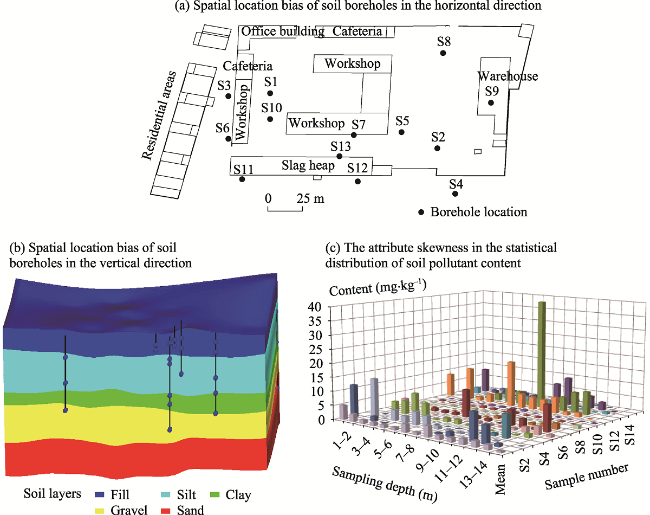
Figure 2 Highly biased characteristics of soil boring at contaminated sites
Affected by the superposition of the natural background and substantial interference from industrial activities, there are abnormal but actual soil boring samples with high pollutant concentrations around samples with low ones (Figure 2c) (Franssen et al., 1997). In order to use the Kriging method to perform statistical inference on the data with high skewness, the normal transformation is generally used to transform the abnormal data into a normal distribution or an approximately normal distribution. Three transformation methods, namely Box-Cox, Rank Order, and Normal Score, are often used to normalize soil pollutant data. The log-normal transformation method is a special one of Box-Cox transformation (Saito and Goovaerts, 2000), which effectively transform the skewed data that conforms to the statistical characteristics of the log-normal distribution. The Rank Order transformation method is suitable for integrating many different types of data sets (Journal and Deutsch, 1997; Juang et al., 2001). The Normal Score transformation method first sorts and grades the raw data set, then finds the corresponding equivalent levels in the standard normal distribution for each level in the raw data set, and finally uses the normal distribution values associated with these levels to form the transformed data set (Deutsch et al., 1998). According to trace elements’ accumulation and migration characteristics in porous soil media, Wu et al. (2011) found that the log-normal distribution transformation better affects the three-dimensional interpolation of topsoil pollutants in a smelter.

4.2 Effect of spatial nonstationary concentration field on the site pollution delineation

Due to the coexistence of autocorrelation (Tobler, 1970) and heterogeneity (Anselin, 1995) of spatial data, the strict second-order stationarity assumption is usually challenging to be satisfied. The three-dimensional distribution of polluted soil is affected by the interaction of multiple factors such as gravity field (MacDonald et al., 2000), topography (Liu et al., 2017), soil texture (Li et al., 2022), and the production layout (Tao et al., 2019) on the ground, which makes the pollutant concentration field at the contaminated sites appear nonstationary. According to the statistical characteristics, spatial nonstationarity includes mean and variance nonstationarity (Myers, 1989; Sampson and Guttorp, 1992; Cuba et al., 2012; Wadoux et al., 2018). This paper divides the nonstationary pollutant concentration field into three typical types: trend nonstationarity, anisotropy nonstationarity, and heterogeneity nonstationarity (Ge et al., 2019).

4.2.1 Spatial trend nonstationarity of concentration field

Spatial trend nonstationary means that the mean of non-homogeneity geographic variables has a spatial trend in space. It can be fitted by global or local polynomial trend surface (or depth functions), such as universal Kriging and three-dimensional interpolation based on depth functions (Ma et al., 2021). It can also use environmental covariates to simulate spatial trends, such as the regression Kriging method. Affected by the hydrodynamic field, the water flow velocity in the vertical direction is usually slower than that in the horizontal direction in the saturated zone of contaminated sites. Therefore, pollutants spread fast horizontally along with the fluid flow. Figure 3 shows the fitting results of pollutants using a local polynomial trend surface at a coking site affected by a groundwater hydrodynamic field in the saturated zone. The delineation accuracy can be improved when delineating the three-dimensional distribution of soil pollutants at contaminated sites by eliminating the fitting trend.
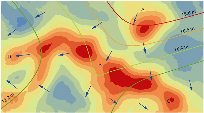
Figure 3 Spatial trend nonstationarity of concentration field influenced by the flow field of underground water

Note: The water table at A is higher than at B, C, and D, resulting in groundwater flow from A to C and D.

4.2.2 Spatial anisotropy nonstationarity of concentration field

Anisotropy is a conception relative to isotropy, which means that geographic variables show different variations in different directions. The value of the variation function is related to the distance and direction between point pairs. The variation of anisotropy can be divided into geometric anisotropy and band anisotropy according to the variables’ natural properties (Eriksson et al., 2000). Geometric anisotropy has the same sill value but different range values in all directions, so it is also called range anisotropy. The variability differences in different directions can be described by the ratio of the range values, namely, the anisotropic ratio coefficient. Ratio transformation is commonly used in practical applications of converting anisotropy to isotropy for ease of understanding. Affected by the coupling of the gravity field and the hydrodynamic field, the variability of the pollutant content within porous soil medium in the vertical direction is larger than that in the horizontal direction (Šichorová et al., 2004); that is, during interpolation, the predicted values of the point pairs in the horizontal direction are more correlated than that in the vertical direction with the sample distance (Figure 4). In the practical application of site pollution delineation, the anisotropic in the vertical and horizontal directions caused by the gravity field can be converted into an isotropic concentration field using an anisotropy ratio coefficient, i.e., the ratio of range value (Tao et al., 2019).
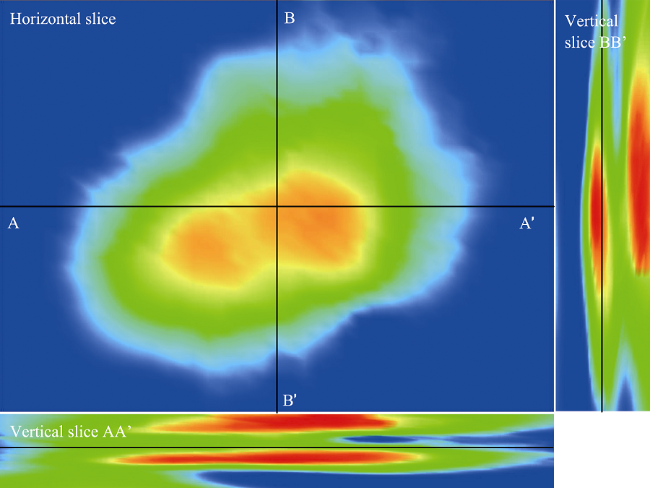
Figure 4 Anisotropy nonstationarity of concentration field in horizontal and vertical directions

4.2.3 Spatial heterogeneity nonstationarity of concentration field

Spatial heterogeneity nonstationarity exhibits the strongest non-homogeneity, referring to the spatial nonstationarity of the variance of geographic variables. It comprises spatial nonstationarity of local heterogeneity and stratification (or partition) heterogeneity (Lark et al., 2009; Wang et al., 2017). The potential point sources in the surface production function area or underground tank led to the nonstationary local spatial heterogeneity. If this spatial heterogeneity can be fitted with a trend surface, it can be classified as a nonstationary local spatial trend. The spatial nonstationarity of stratification heterogeneity at contaminated sites means that the pollutant concentration field is globally nonstationary but keeps relatively stationary in the sub-regions of the stratification (Marchant et al., 2009; Gao et al., 2015). Therefore, it can be transformed into spatial stationarity by spatially dividing the sub-regions. There are great differences in soil pollutants’ migration ability and accumulation in different soil layers.
Taking the three-dimensional delineation of dense non-aqueous phase liquid (DNAPL) as an example (Figure 5), it is easy to migrate vertically for DNAPL pollutants. However, if there is an impermeable layer, such as a clay layer, at the contaminated site, it will significantly affect the vertical migration ability of DNAPL. Consequently, DNAPL will be enriched in the impermeable layer. If we ignore the effect of the spatial stationarity of stratification heterogeneity of the soil layers when fitting the three-dimensional semivariogram of DNAPL, it will be unfaithful to describe the three-dimensional structure of DNAPL. In the practical application of site pollution delineation, the hierarchical Kriging integrating the prior knowledge of soil layer information at contaminated sites can be developed under the Bayesian framework (Liu et al., 2021).
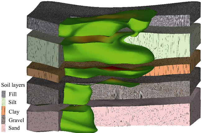
Figure 5 Heterogeneous nonstationarity of concentration field of DNAPL influenced by soil textures
Large-scale and complex contaminated sites have the characteristics of deep polluted soil mass and large vertical variation of pollutants’ content in different soil textures. In a large-scale and complex contaminated site, the above three types of nonstationary do not exist separately. Multiple types of nonstationarity of pollutant concentration fields are usually coupled. For example, certain nonstationarity is the coupling result of spatial trend nonstationarity and anisotropic nonstationarity. For another example, there are stationarity, spatial trend nonstationarity, and anisotropic nonstationarity in the same sub-region of hierarchical heterogeneous nonstationarity. Therefore, for spatial nonstationary concentration fields of large-scale and complex contaminated sites, it is necessary to examine the three- imensional site pollution delineation model that couples multiple nonstationary situations.

5 Conclusion and prospects

Scientific diagnosis and effective control of pollution risks at contaminated sites have become the key to soil pollution control in China. Many contaminated sites are located in the new-type urbanization areas, which puts forward higher requirements for fine risk management and control strategies at contaminated sites to support accurate three-dimensional delineation information. However, a contaminated site is a three-dimensional complex system coupled with multiple elements above- and under-ground, and pollutants in this three-dimensional complex system have the characteristics of strong spatial heterogeneity and concealment, both of which impede the practical application of three-dimensional discrete data collected by soil boring to delineate the pollutants. Furthermore, it is difficult to directly introduce the relatively mature three-dimensional delineation models of offshore and petroleum exploration into site pollution delineation. The interpolation theory and methods in spatial statistics have recently made significant progress. So does the application of holographic visualization technology to three-dimensional complicated geological mass. That progress provides new means for the site pollution delineation.
At present, extensive research verified the spatial statistics in the two-dimensional interpolation of soil pollutant content, data correction of soil samples, uncertainty calculation of interpolation results, and optimization of soil sampling. Some of these theories and methods are maturing. However, we have to address the problems of sparse borehole sites, biased samples, deep polluted soil mass, and spatially nonstationary pollutant concentration field for the three-dimensional site pollution delineation. These problems incur the poor data representation and reproducibility for pollutants content data collected by a discrete three-dimensional borehole (Kedron and Holler, 2022) and high uncertainty in the site pollution delineation when applying the current theories and methods. In the future, the research on the site pollution delineation can make breakthroughs in the following six aspects: multi-scenario, nonstationary, nonlinear, multi-source data fusion, multi-type model coupling, and combined pollution characterization, to realize the transparency of underground “black box” soil pollution and improve the scientific diagnosis and fine management level of pollution risks at contaminated sites.

5.1 Shift toward the site pollution delineation methodology in multi-scenarios from a single-scenario

The hydrogeological condition of the contaminated site is complex, and the borehole layouts are various. In the scenarios of spatial representation of different borehole sites, it is necessary to quantitatively describe the spatial bias of the sparse samples to realize the identification and measurement of the statistical characteristics of soil boring samples in different scenarios. In addition, there are various types of pollutants at contaminated sites, and their migration abilities are different. It is necessary to decouple the mean nonstationarity and variance nonstationary from pollutant concentration fields and then develop a set of indicators to measure them. A set of site pollution delineation methodology under multi-scenario conditions should be developed for the spatial bias of soil boring data, various pollutant types, and different nonstationary types of pollutant concentration fields.

5.2 Shift toward nonstationary three-dimensional site pollution delineation method from the stationary method

In the current research on the site pollution delineation of soil pollution, the spatial statistics models represented by geostatistical methods all require the soil pollutant concentration field to satisfy strict second-order stationary or intrinsic assumptions. However, it is difficult to satisfy this assumption when pollutant concentration fields are influenced by strong industrial activities and complex hydrogeological conditions. Therefore, the fitted semivariogram is insufficient to accurately describe the spatial structure of soil pollutants, which results in the problem of high uncertainty in site pollution delineation (Li et al., 2007). In the future, the improvement of nonstationary site pollution delineation could start in the following two ways. On the one hand, the nonstationary spatial interpolation can be transformed into a stationary interpolation, such as detrend or deformation transformation. On the other hand, a site pollution delineation model without stationary assumptions can be directly constructed, such as indicator Kriging or disjunctive Kriging.

5.3 Shift toward nonlinear three-dimensional delineation model from the linear model

Affected by the local complex hydrogeological conditions at contaminated sites, the migration characteristics of soil pollutants in three-dimensional space are difficult to be captured by linear spatial statistic methods. Methods such as machine learning under the Bayesian framework (Quach et al., 2017; Fuentes et al., 2020) or deep learning (Samui and Sitharm, 2010; Man et al., 2022; Zhan et al., 2022) should be developed, which can effectively improve the characterization accuracy. In particular, the convolutional neural network interpolation methods such as graph neural network (GNN) and confrontation generative neural network (GAN) have emerged in the field of geographic artificial intelligence (GeoAI) in recent years (Zhu et al., 2020; Zhu et al., 2021; Zheng et al., 2022) are promising for solving the problem of site pollution delineation in a complex geological mass environment.

5.4 Shift toward multi-source data fusion of surface, above- and under-ground from discrete soil boring data

The single soil boring data in geographical space has the shortcoming of spatial bias and spatial nonstationary of concentration field. Thus, further research on the site pollution delineation should be central to the feature space. Future research should integrate multi-source uncertainty data of temperature field, gravity field, hydrodynamic field, and electromagnetic signal at contaminated sites (Kang et al., 2020; Zeng et al., 2022a) and examine the fine site pollution delineation considering the spatial heterogeneity of soil pollutants, the migration law of soil pollutants, and the physical and chemical properties of soil under the Bayesian framework. For example, we can extend existing co-Kriging, regression Kriging, empirical Bayesian Kriging method from two dimensions to three dimensions (Krivoruchko and Griboc, 2019; Griboc and Krivoruchko, 2020).

5.5 Shift toward the combination of spatial statistics and mechanism models from single geostatistics

The site pollution delineation based on geostatistical methods can provide the inference results of linear unbiased and optimal, but the delineation results rely too much on the data structure of soil boring samples. The geostatistics method has low delineation accuracy when borehole samples are sparse and biased. For another, the mechanism model can achieve high delineation accuracy when fully considering the complex kinetic process of the pollutant solute migration, and a large number of model parameters used to define the initial and boundary conditions need to be obtained and corrected. However, these parameters are expensive to acquire and will introduce uncertainties that are difficult to estimate. Integrating the simulation results of the geostatistical model and the mechanism model needs to combine the migration mechanism of soil pollutants with the spatial statistics, which can overcome the shortcomings of the traditional single spatial statistic prediction and reduce the investigation cost (Shlomi and Michalak, 2007).

5.6 Shift toward site characterization of combined pollutants from single pollutant

Some of the current industrial contaminated sites are large-scale and complex sites with the characteristics of covering a large area, involving many industries, having many types of pollutants of concern, and having high pollution risks. When carrying out site pollution delineation of large-scale and complex sites, it is necessary to pay attention to the accuracy test of the delineation results for combined pollutants, analyze the sources of delineation errors, and the law of propagation of error. On that basis, decision-makers need further evaluate the fitness of the constructed site pollution delineation models for combined pollutants by analyzing the population characteristics and the statistical distribution of borehole samples of different pollutants (Boudreault et al., 2016; Tao et al., 2019).
[1]
Anselin L, 1995. Local indicators of spatial association: LISA. Geographical Analysis, 27(2): 93-115.

DOI

[2]
Boudreault J P, Dubé J S, Marcotte D, 2016. Quantification and minimization of uncertainty by geostatistical simulations during the characterization of contaminated sites: 3-D approach to a multi-element contamination. Geoderma, 264: 214-226.

DOI

[3]
Brus D J, de Gruijter J J, 1997. Random sampling or geostatistical modelling? Choosing between design-based and model-based sampling strategies for soil (with discussion). Geoderma, 80: 1-40.

DOI

[4]
Brus D J, Yang L, Zhu A X, 2019. Accounting for differences in costs among sampling locations in optimal stratification. European Journal of Soil Science, 70(1): 200-212.

DOI

[5]
Brus D J, Yang R M, Zhang G L, 2016. Three-dimensional geostatistical modeling of soil organic carbon: A case study in the Qilian Mountains, China. CATENA, 141: 46-55.

DOI

[6]
Campbell J E, Moen J C, Ney R A et al., 2008. Comparison of regression coefficient and GIS-based methodologies for regional estimates of forest soil carbon stocks. Environmental Pollution, 152(2): 267-273.

PMID

[7]
Cao G, Yang L, Liu L, et al., 2018. Environmental incidents in China: Lessons from 2006 to 2015. Science of the Total Environment, 633: 1165-1172.

DOI

[8]
Chadalavada S, Datta B, Naidu R, 2011. Uncertainty based optimal monitoring network design for a chlorinated hydrocarbon contaminated site. Environmental Monitoring and Assessment, 173(1): 929-940.

DOI

[9]
Chen X, Murakami H, Hahn M S et al., 2012. Three-dimensional Bayesian geostatistical aquifer characterization at the Hanford 300 Area using tracer test data. Water Resources Research, 48(6): w06501.

[10]
Cuba M A, Leuangthong O, Ortiz J M, 2012. Detecting and quantifying sources of nonstationarity via experimental semivariogram modeling. Stochastic Environmental Research and Risk Assessment, 26(2): 247-260.

DOI

[11]
Deutsch C V, Journel A G, 1998. GSLIB, Geostatistical Software Library and User’s Guide. New York: Oxford University Press.

[12]
Eriksson M, Siska P P, 2000. Understanding anisotropy computations. Mathematical Geology, 32(6): 683-700.

DOI

[13]
Fang C, Zhou C, Gu C et al., 2017. A proposal for the theoretical analysis of the interactive coupled effects between urbanization and the eco-environment in mega-urban agglomerations. Journal of Geographical Sciences, 27(12): 1431-1449.

DOI

[14]
Franssen H J W M H, Eijnsbergen A C V, Stein A, 1997. Use of spatial prediction techniques and fuzzy classification for mapping soil pollutants. Geoderma, 77: 243-262.

DOI

[15]
Fuentes I, Padarian J, Iwanaga T et al., 2020. 3D lithological mapping of borehole descriptions using word embeddings. Computers & Geosciences, 141: 104516.

DOI

[16]
Gao B B, Liu Y, Pan Y et al., 2017. Error index for additional sampling to map soil contaminant grades. Ecological Indicators, 77: 129-138.

DOI

[17]
Gao B B, Wang J F, Fan H M et al., 2015. A stratified optimization method for a multivariate marine environmental monitoring network in the Yangtze River estuary and its adjacent sea. International Journal of Geographical Information Science, 29(8): 1332-1349.

DOI

[18]
Ge Y, Jin Y, Stein A et al., 2019. Principles and methods of scaling geospatial Earth science data. Earth Science Reviews, 197: 102897.

DOI

[19]
Goovaerts P, 1999. Geostatistics in soil science: State-of-the-art and perspectives. Geoderma, 89(1/2): 1-45.

DOI

[20]
Grauer-Gray J, Hartemink A E, 2018. Raster sampling of soil profiles. Geoderma, 318: 99-108.

DOI

[21]
Gribov A, Krivoruchko K, 2020. Empirical Bayesian kriging implementation and usage. Science of the Total Environment, 722: 137290. doi: 10.1016/j.scitotenv.2020.137290.

DOI

[22]
Guo G L, Wang X, G L et al., 2009. Site-specific spatial distribution of VOC/SVOC and determination of the remediation boundary. Acta Scientiae Circumstantiae, 29(12): 2597-2605. (in Chinese)

[23]
Haskard K A, Lark R M, 2009. Modelling nonstationary variance of soil properties by tempering an empirical spectrum. Geoderma, 153(1/2): 18-28.

DOI

[24]
Jiang C S, Wang J F, Cao Z D, 2009. A review of geo-spatial sampling theory. Acta Geographica Sinica, 64(3): 368-380. (in Chinese)

DOI

[25]
Jiang S J, Wang J S, Zhai Y Z et al., 2016. Determination of the volume of soil requiring remediation in contaminated sites based on conditional simulation. Acta Scientiae Circumstantiae, 36(7): 2596-2604. (in Chinese)

[26]
Jones N L, Davis R J, 1996. Three-dimensional characterization of contaminant plumes. Transportation Research Record, 1526(1): 177-182.

DOI

[27]
Jones N L, Davis R J, Sabbah W, 2003. A comparison of three-dimensional interpolation techniques for plume characterization. Groundwater, 41(4): 411-419. doi: 10.1111/j.1745-6584.2003.tb02375.x.

DOI PMID

[28]
Journel A G, Deutsch C V, 1997. Rank order geostatistics: A proposal for a unique coding and common processing of diverse data. Geostatistics Wollongong, 96(1): 174-187.

[29]
Juang K W, Lee D Y, Ellsworth T R, 2001. Using rank-order geostatistics for spatial interpolation of highly skewed data in a heavy-metal contaminated site. Journal of Environmental Quality, 30(3): 894-903.

PMID

[30]
Juang K W, Liao W J, Liu T L et al., 2008. Additional sampling based on regulation threshold and kriging variance to reduce the probability of false delineation in a contaminated site. Science of the Total Environment, 389(1): 20-28.

DOI

[31]
Kang X, Kokkinaki A, Kitanidis P K et al., 2020. Improved characterization of DNAPL source zones via sequential hydrogeophysical inversion of hydraulic-head, self-potential and partitioning tracer data. Water Resources Research, 56(8): e2020WR027627.

[32]
Kedron P, Holler J, 2022. Replication and the search for the laws in the geographic sciences. Annals of GIS, 28(1): 45-56.

DOI

[33]
Krivoruchko K, Gribov A, 2019. Evaluation of empirical Bayesian Kriging. Spatial Statistics, 32: 100368.

DOI

[34]
Lacoste M, Minasny B, McBratney A et al., 2014. High resolution 3D mapping of soil organic carbon in a heterogeneous agricultural landscape. Geoderma, 213: 296-311.

DOI

[35]
Lark R M, 2009. Kriging a soil variable with a simple nonstationary variance model. Journal of Agricultural, Biological, and Environmental Statistics, 14(3): 301-321.

[36]
Li F, Yan Z, 2009. Vocabulary Handbook of Contaminated Sites. Beijing: Science Press. (in Chinese)

[37]
Li J, Heap A D, 2014. Spatial interpolation methods applied in the environmental sciences: A review. Environmental Modelling & Software, 53: 173-189.

[38]
Li K B, Goovaerts P, Abriola L M, 2007. A geostatistical approach for quantification of contaminant mass discharge uncertainty using multilevel sampler measurements. Water Resources Research, 43(6): w06436.

[39]
Li X X, Zhang B, Wan Z M et al., 2017. Application of Golden Software Voxler in the investigation and health risk assessment for contaminated site. Science Technology and Engineering, 17(8): 322-328. (in Chinese)

[40]
Li Z, Tao H, Zhao D, et al., 2022. Three-dimensional empirical Bayesian Kriging for soil PAHs interpolation considering the vertical soil lithology. CATENA, 212: 106098.

DOI

[41]
Liao Q, Deng Y, Shi X, et al., 2018a. Delineation of contaminant plume for an inorganic contaminated site using electrical resistivity tomography: Comparison with direct-push technique. Environmental Monitoring and Assessment, 190(4): 187.

DOI

[42]
Liao X Y, Chong Z Y, Yan X L, et al., 2011. A new issue in the field of environmental remediation in China. Environmental Science, 32(3): 784-794. (in Chinese)

[43]
Liao Y, Li D, Zhang N, 2018b. Comparison of interpolation models for estimating heavy metals in soils under various spatial characteristics and sampling methods. Transactions in GIS, 22(2): 409-434.

DOI

[44]
Liu F, Zhang G L, Sun Y J et al., 2013b. Mapping the three-dimensional distribution of soil organic matter across a subtropical hilly landscape. Soil Science Society of America Journal, 77(4): 1241-1253.

DOI

[45]
Liu G, Bi R, Wang S et al., 2013a. The use of spatial autocorrelation analysis to identify PAHs pollution hotspots at an industrially contaminated site. Environmental Monitoring and Assessment, 185(11): 9549-9558.

DOI

[46]
Liu G, Niu J, Guo W et al., 2017. Assessment of terrain factors on the pattern and extent of soil contamination surrounding a chemical industry in Chongqing, Southwest China. CATENA, 2017, 156: 237-243.

DOI

[47]
Liu G, Niu J, Zhang C et al., 2015. Accuracy and uncertainty analysis of soil Bbf spatial distribution estimation at a coking plant-contaminated site based on normalization geostatistical technologies. Environmental Science and Pollution Research, 22(24): 20121-20130.

DOI

[48]
Liu G, Niu J J, Zhang C et al., 2014. Spatial distribution prediction of surface soil Pb in a battery contaminated site. Environmental Science, 35(12): 4712-4719. (in Chinese)

[49]
Liu G, Zhou X, Li Q et al., 2020. Spatial distribution prediction of soil As in a large-scale arsenic slag contaminated site based on an integrated model and multi-source environmental data. Environmental Pollution, 267: 115631.

DOI

[50]
Liu Y, Chen Y, Wu Z et al., 2021. Geographical detector-based stratified regression kriging strategy for mapping soil organic carbon with high spatial heterogeneity. CATENA, 196: 104953.

DOI

[51]
Ma Y, Minasny B, McBratney A et al., 2021. Predicting soil properties in 3D: Should depth be a covariate? Geoderma, 383: 114794.

DOI

[52]
MacDonald L A, 2000. Sub-surface migration of an oil pollutant into aquifers[D]. Plymouth: University of Plymouth.

[53]
Man J, Zeng L, Luo J et al., 2022. Application of the deep learning algorithm to identify the spatial distribution of heavy metals at contaminated sites. ACS ES&T Engineering, 2(2): 158-168.

[54]
Marchant B P, McBratney A B, Lark R M et al., 2013. Optimized multi-phase sampling for soil remediation surveys. Spatial Statistics, 4: 1-13.

DOI

[55]
Marchant B P, Newman S, Corstanje R et al., 2009. Spatial monitoring of a nonstationary soil property: phosphorus in a Florida water conservation area. European Journal of Soil Science, 60: 757-769.

DOI

[56]
Matheron G, 1963. Principles of geostatistics. Economic Geology, 58: 1246-1266.

DOI

[57]
McIntyre E, Prior J, Connon I L C, et al., 2018. Sociodemographic predictors of residents worry about contaminated sites. Science of the Total Environment, 643: 1623-1630.

DOI

[58]
Men X Y, Yang Z Z, Liu X et al., 2017. Application of 3-D spatial interpolation technique to analyzing the distribution of TPH contamination in a field-site. Journal of Safety and Environment, 17(2): 713-718. (in Chinese)

[59]
Minasny B, McBratney A B, 2006. A conditioned Latin hypercube method for sampling in the presence of ancillary information. Computers and Geosciences, 32(9): 1378-1388.

DOI

[60]
Minasny B, McBratney A B, Walvoort D J J, 2007. The variance quadtree algorithm: Use for spatial sampling design. Computers & Geosciences, 33(3): 383-392.

DOI

[61]
Myers D E, 1989. To be or not to be stationary? That is the question. Mathematical Geology, 21(3): 347-362.

DOI

[62]
Pan Y, Ren X, Gao B et al., 2015. Global mean estimation using a self-organizing dual-zoning method for preferential sampling. Environmental Monitoring & Assessment, 187(3): 187-121.

[63]
Pannecoucke L, Le Coz M, Freulon X et al., 2020. Combining geostatistics and simulations of flow and transport to characterize contamination within the unsaturated zone. Science of the Total Environment, 699: 134216.

DOI

[64]
Perroy R L, Belby C S, Mertens C J, 2014. Mapping and modeling three dimensional lead contamination in the wetland sediments of a former trap-shooting range. Science of the Total Environment, 487: 72-81.

DOI

[65]
Poggio L, Gimona A, 2014. National scale 3D modelling of soil organic carbon stocks with uncertainty propagation: An example from Scotland. Geoderma, 232: 284-299.

[66]
Quach A N O, Tabor L, Dumont D et al., 2017. A machine learning approach for characterizing soil contamination in the presence of physical site discontinuities and aggregated samples. Advanced Engineering Informatics, 33: 60-67.

DOI

[67]
Ren L, Lu H, He L et al., 2016. Characterization of monochlorobenzene contamination in soils using geostatistical interpolation and 3D visualization for agrochemical industrial sites in southeast China. Archives of Environmental Protection, 42(3): 17-24.

DOI

[68]
Saito H, Goovaerts P, 2000. Geostatistical interpolation of positively skewed and censored data in a dioxin-contaminated site. Environmental Science & Technology, 34: 4228-4235.

DOI

[69]
Sampson P D, Guttorp P, 1992. Nonparametric-estimation of nonstationary spatial covariance structure. Journal of the American Statistical Association, 87: 108-119.

DOI

[70]
Samui P, Sitharam T G, 2010. Site characterization model using artificial neural network and Kriging. International Journal of Geomechanics, 10(5): 171-180.

DOI

[71]
Schnabel U, Tietje O, Scholz R W, 2004. Uncertainty assessment for management of soil contaminants with sparse data. Environmental Management, 33(6): 911-925. doi: 10.1007/s00267-003-2971-0.

DOI PMID

[72]
Shlomi S, Michalak A M, 2007. A geostatistical framework for incorporating transport information in estimating the distribution of a groundwater contaminant plume. Water Resources Research, 43(3): w03412.

[73]
Šichorová K, Tlustoš P, Száková J et al., 2004. Horizontal and vertical variability of heavy metals in the soil of a polluted area. Plant Soil and Environment, 50(12): 523-534.

[74]
Tao H, Liao X Y, Yan X L et al., 2014. Uncertainty analysis and pollution volumetric calculation of soil BaP contents in a contaminated site. Geographical Research, 33(10): 1857-1865. (in Chinese)

DOI

[75]
Tao H, Liao X Y, Yan X L et al., 2017. Methodological investigation on dynamically adding samples for drilling design in contaminated site investigation. Acta Scientiae Circumstantiae, 37(4): 1461-1468. (in Chinese)

[76]
Tao H, Liao X Y, Zhao D, et al., 2019. Delineation of soil contaminant plumes at a co-contaminated site using BP neural networks and geostatistics. Geoderma, 354(15): 113878.

DOI

[77]
Tobler W R, 1970. A computer movie simulating urban growth in the Detroit region. Economic Geography, 46(2): 234-240.

DOI

[78]
Troldborg M, Nowak W, Lange I V et al., 2012. Application of Bayesian geostatistics for evaluation of mass discharge uncertainty at contaminated sites. Water Resources Research, 48(9): w09535.

[79]
van Meirvenne M, Goovaerts P, 2001. Evaluating the probability of exceeding a site-specific soil cadmium contamination threshold. Geoderma, 102(1/2): 75-100.

DOI

[80]
Veronesi F, Corstanje R, Mayr T, 2012. Mapping soil compaction in 3D with depth functions. Soil and Tillage Research, 124: 111-118.

DOI

[81]
Verstraete S, Van Meirvenne M, 2008. A multi-stage sampling strategy for the delineation of soil pollution in a contaminated brownfield. Environmental Pollution, 154(2): 184-191.

PMID

[82]
Volchko Y, Kleja D B, Back P E et al., 2020. Assessing costs and benefits of improved soil quality management in remediation projects: A study of an urban site contaminated with PAH and metals. Science of The Total Environment, 707: 135582.

DOI

[83]
Wadoux A M J C, Brus D J, Heuvelink G B M, 2018. Accounting for nonstationary variance in geostatistical mapping of soil properties. Geoderma, 324: 138-147.

DOI

[84]
Wang J F, Haining R, Cao Z D, 2010. Sample surveying to estimate the mean of a heterogeneous surface: reducing the error variance through zoning. International Journal of Geographical Information Science, 24(4): 523-543.

DOI

[85]
Wang J F, Stein A, Gao B B et al., 2012. A review of spatial sampling. Spatial Statistics, 2: 1-14.

DOI

[86]
Wang J F, Xu C D. 2017. Geodetector: Principle and prospective. Acta Geographica Sinica, 72(1): 116-134. (in Chinese)

DOI

[87]
Wu C, Wu J, Luo Y et al., 2011. Spatial interpolation of severely skewed data with several peak values by the approach integrating Kriging and triangular irregular network interpolation. Environmental Earth Sciences, 63(5): 1093-1103.

DOI

[88]
Xie Y F, Chen T B, Lei M, et al., 2011. Spatial distribution of soil heavy metal pollution estimated by different interpolation methods: Accuracy and Uncertainty Analysis. Chemosphere, 82(3): 468-476.

DOI PMID

[89]
Xu C D, Wang J F, Li Q X, 2018. A new method for temperature spatial interpolation based on sparse historical stations. Journal of Climate, 31(5): 1757-1770.

DOI

[90]
Yihdego Y, Al-Weshah R A, 2016. Gulf war contamination assessment for optimal monitoring and remediation cost-benefit analysis, Kuwait. Environmental Earth Sciences, 75(18): 1234.

DOI

[91]
Zeng J, Li C, Wang J et al., 2022a. Pollution simulation and remediation strategy of a zinc smelting site based on multi-source information. Journal of Hazardous Materials, 433(5): 128774.

DOI

[92]
Zeng J, Luo X, Cheng Y et al., 2022b. Spatial distribution of toxic metal (loid) s at an abandoned zinc smelting site, southern China. Journal of Hazardous Materials, 425: 127970.

DOI

[93]
Zhan C, Dai Z, Soltanian M R et al., 2022. Stage-wise stochastic deep learning inversion framework for subsurface sedimentary structure identification. Geophysical Research Letters, 49(1): e2021GL095823.

[94]
Zhang Y, Ji W, Saurette D D et al., 2020. Three-dimensional digital soil mapping of multiple soil properties at a field-scale using regression kriging. Geoderma, 366: 114253.

DOI

[95]
Zhao Y S, Liao X Y, Li Y et al., 2019. Occurrence characteristics and health risks of PAHs on the surface of buildings and devices in the coking plant. Environmental Sciences, 40(11): 4870-4878. (in Chinese)

[96]
Zheng S, Wang J, Zhuo Y et al., 2022. Spatial distribution model of DEHP contamination categories in soil based on Bi-LSTM and sparse sampling. Ecotoxicology and Environmental Safety, 229: 113092.

DOI

[97]
Zhu D, Cheng X, Zhang F et al., 2020. Spatial interpolation using conditional generative adversarial neural networks. International Journal of Geographical Information Science, 34(4): 735-758.

DOI

[98]
Zhu D, Liu Y, Yao X et al., 2021. Spatial regression graph convolutional neural networks: A deep learning paradigm for spatial multivariate distributions. GeoInformatica: 1-32.

Outlines

/