Research Articles

Traffic accessibility and the coupling degree of ecosystem services supply and demand in the middle reaches of the Yangtze River urban agglomeration, China

  • CHEN Wanxu , 1, 2 ,
  • BIAN Jiaojiao 1 ,
  • LIANG Jiale 3 ,
  • PAN Sipei 3 ,
  • ZENG Yuanyuan 4
Expand
  • 1. Department of Geography, School of Geography and Information Engineering, China University of Geosciences, Wuhan 430074, China
  • 2. State Key Laboratory of Earth Surface Processes and Resource Ecology, Beijing Normal University, Beijing 100875, China
  • 3. School of Public Administration, China University of Geosciences, Wuhan 430074, China
  • 4. 4th Planning & Design Office, Guangdong Urban & Rural Planning and Design Institute, Guangzhou 510290, China

Chen Wanxu (1989-), PhD, specialized in resource and environment assessment and regional economic analysis. E-mail:

Received date: 2021-07-29

  Accepted date: 2021-12-22

  Online published: 2022-10-25

Supported by

National Natural Science Foundation of China(42001187)

National Natural Science Foundation of China(41701629)

Abstract

The spatial relationships between traffic accessibility and supply and demand (S&D) of ecosystem services (ESs) are essential for the formulation of ecological compensation policies and ESs regulation. In this study, an ESs matrix and coupling analysis method were used to assess ESs S&D based on land-use data for 2000, 2010, and 2020, and spatial regression models were used to analyze the correlated impacts of traffic accessibility. The results showed that the ESs supply and balance index in the middle reaches of the Yangtze River urban agglomeration (MRYRUA) continuously decreased, while the demand index increased from 2000 to 2020. The Gini coefficients of these indices continued to increase but did not exceed the warning value (0.4). The coupling degree of ESs S&D continued to increase, and its spatial distribution patterns were similar to that of the ESs demand index, with significantly higher values in the plains than in the montane areas, contrasting with those of the ESs supply index. The results of global bivariate Moran’s I analysis showed a significant spatial dependence between traffic accessibility and the degree of coupling between ESs S&D; the spatial regression results showed that an increase in traffic accessibility promoted the coupling degree. The present results provide a new perspective on the relationship between traffic accessibility and the coupling degree of ESs S&D, representing a case study for similar future research in other regions, and a reference for policy creation based on the matching between ESs S&D in the MRYRUA.

Cite this article

CHEN Wanxu , BIAN Jiaojiao , LIANG Jiale , PAN Sipei , ZENG Yuanyuan . Traffic accessibility and the coupling degree of ecosystem services supply and demand in the middle reaches of the Yangtze River urban agglomeration, China[J]. Journal of Geographical Sciences, 2022 , 32(8) : 1471 -1492 . DOI: 10.1007/s11442-022-2006-5

1 Introduction

As a mobile carrier of national economy, transportation infrastructure connects production and consumption, balances regional supply and demand (S&D), and plays a role in attracting, producing, and agglomerating industries, capital, and populations (Jin and Chen, 2019). Urban agglomerations are the highest form of spatial organization in the mature stages of urban development (Fang and Yu, 2017). Relying on developed infrastructure networks such as transportation and communication, urban agglomerations form close economic ties, with a high degree of urban homogenization and integration in relatively compact spatial units (Fang et al., 2018). Traffic accessibility plays an important role in the formation and development of urban agglomerations, as well as in the evolution of the relationship between the S&D of ecosystem services (ESs). However, previous research has neglected the impact of traffic accessibility on the S&D of ESs in urban agglomerations. It is of great practical significance to address issues related to the rapid development of transportation infrastructure and the mismatch between ESs S&D in urban agglomerations. Therefore, it is necessary to explore the influence mechanism of traffic accessibility on the ESs S&D.
Maintaining the balance between S&D of ESs is the guarantee and key to the safe and healthy development of ecosystems (Jing et al., 2018). Many scholars have explored the spatial patterns (González-García et al., 2020; Sun et al., 2020; Xu et al., 2021), tradeoffs (Liu et al., 2022), spatially heterogeneity (Pan and Wang, 2021), spatial disparities (Yu et al., 2021), services flow (Feurer et al., 2021), driving evolution mechanisms of ESs S&D, mainly including socio-economic and physical factors (Spake et al., 2017; Tao et al., 2018; Zhang et al., 2018; Cao et al., 2021). However, ESs S&D in previous studies were often regarded as two independent variables, thereby ignoring the coupling relationships between them (Xu et al., 2022). Moreover, few studies have revealed the interaction mechanism between traffic accessibility and the coupling degree of ESs S&D at 5 km and 10 km scales (Mehring et al., 2018). In addition, when choosing the research method, the non-spatial regression models ignore the spatial dependence effect, and thus cannot fully explain the effect of traffic accessibility on the coupling degree of ESs S&D (Chen et al., 2020a). However, spatial regression models consider spatial lag and error and can effectively compensate for this limitation.
Identifying the impacts of traffic accessibility on the coupling degree of ESs S&D can offer an in-depth perspective to alleviate the current issues faced by urban agglomerations, for example, the tightening of urban sprawl, resource constraints, and problems such as degraded ecosystem functions. To this end, the present research selected the middle reaches of the Yangtze River urban agglomeration (MRYRUA), China, as a case study to explore the spatiotemporal characteristics of regional traffic accessibility and ESs S&D, as well as its influential mechanisms on correlated coupling relationships. MRYRUA is an important component of Chinese national strategies, including the Yangtze River Economic Belt Strategy, Central China Rising Strategy, and the Triangle of Central China (Chen et al., 2020a). Land use in the MRYRUA has undergone a profound transition, bringing about a significant ecological impact throughout the process of rapid development in the past decades (Chen et al., 2020b, 2021).
Accordingly, three objectives were set in this study: (1) estimating the spatiotemporal patterns of ESs S&D at 5 and 10 km scales in the MRYRUA; (2) measuring the coupling degree of ESs S&D in the MRYRUA; and (3) identifying the multi-scale differences in the impact of traffic accessibility on the coupling degree of ESs S&D. These goals were approached in an effort to deepen the theoretical understanding of the intrinsic relationship between traffic accessibility and the coupling degree of ESs S&D, provide a reference for decision- and policy-making regarding high-quality development and differentiated regulatory measures in urban agglomerations that emphasize ecosystem protection, and provide references for similar areas in other fast-growing urban agglomeration concentration areas.

2 Literature review

2.1 Traffic accessibility

Traffic elements are an important driving factor of land use changes, which have an important impact on urban spatial morphology, land development speed, and land use market (Zeng et al., 2018; Zhu et al., 2019; Hu et al., 2021). Accessibility is the main effect of a traffic system influencing spatial developments and settlement as calculated in the real estate-, residential location-, and firm location modules (Zondag et al., 2015). Traffic accessibility is an important indicator for measuring the regional traffic network structure and reflecting the actual traffic location conditions (Yang, 2017). It was first proposed as a quantitative index representing regional traffic conditions by Hansen (1959). Traffic accessibility can directly impact the regional economic level, and it is a valuable reference point for regional industrial arrangements and traffic planning (Gulyás and Kovács, 2016; Zhang et al., 2019). Currently, there are mainly two categories of methods for assessing traffic accessibility. The first is to calculate the degree of traffic convenience of a place, including, for example, the density of road networks, the sum of the shortest path from one place to other places in one area, and the average shortest path from one place to other places in one area (Zhang et al., 2019). The second is to measure the probability of people or goods arriving at a certain place, including calculating the weighted average travel time (Gutiérrez, 2001; Zhang et al., 2019) and minimizing travel costs (Meng and Yang, 2002; Zhang et al., 2019).

2.2 Coupling analysis of ecosystem services supply and demand

ESs are obtained by humans directly or indirectly from ecosystems to form and maintain the environmental conditions and utility necessary for survival and development (Costanza et al., 1997; MA, 2005). Flow, supply, and demand are the three basic links of ESs. The movement of ESs from one region to another for anthropogenic use forms ESs flow (Burkhard et al., 2014; Baró et al., 2016; Wang et al., 2021). ESs flow should rely on a carrier, under the influence of natural or human factors, along a certain direction or path towards anthropogenic use areas (Fisher et al., 2009). ESs flow is regarded as the actual supply of ESs (Mononen et al., 2016). Hence, it can dynamically merge with ESs and human demand and solve the problems of ESs value (Fisher and Turner, 2008) and the spatial imbalance in ESs S&D (Brauman et al., 2007). Increasing attention has been paid to human needs in the field of ESs S&D, as by definition, ecosystem structure and processes cannot form ESs without human beneficiaries (Burkhard et al., 2009; Burkhard et al., 2012). ESs supply refers to those products and services produced by environments for human use, whereas ESs demand refers to their consumption and use of said products and services, together forming the dynamic process of ESs flowing from natural ecosystems to social systems (Burkhard et al., 2012; Jing et al., 2018). Recently, considerable research has focused on the balance of ESs S&D and its correlated impact on human welfare based on their capacity to meet these demands in certain regions (Tao et al., 2018; Chen et al., 2020a).

2.3 Impact of traffic accessibility on the coupling degree of ecosystem services

Regional ecological problems are primarily the result of changes to the ecological structure and pattern caused by human activities, which in turn are essentially caused by spatial differences or imbalances in the ESs S&D (Ou et al., 2018; Tao et al., 2018). With the intensification of anthropogenic activities, demand for ESs has increased rapidly interrupting the balance and synergistic relationship between ESs S&D, especially in rapidly developing urban agglomerations (Ou et al., 2018; Chen et al., 2020a). The gradual improvement of traffic networks within urban agglomerations is an important indicator of the formation and development of these intercity clusters. With the rapid development of urbanization and economy in urban agglomerations, their traffic network has gradually improved, thereby impacting the spatial patterns and matching of ESs S&D (Ou et al., 2018; Chen et al., 2020a). Although traffic accessibility plays an important role in the process of matching ESs S&D, few studies have explored its impact on the coupling degree of ESs S&D in urban agglomerations.
The exploration of the impact of traffic accessibility is critical to reveal the differences between ESs S&D, reflect the spatial allocation of resources, and provide theoretical support for ESs payments and compensation mechanisms. ESs flow, as an essential link between ESs S&D, plays an important role in their transport, transformation, and maintenance. The improvement of transportation infrastructure is advantageous to urban residents’ daily lives and economic activities between enterprises. As an important carrier of ESs flow, transportation can relocate primary bodies of energy (Bagstad et al., 2013; Guida-Johnson and Zuleta, 2013) and plays a key role in reshaping the spatial pattern and structure of ESs S&D. Previous studies have shown that improved traffic accessibility can exacerbate the imbalance of ESs (Chen et al., 2020a), such as a bridge connecting previously undisturbed forestland to urban city centers. The coupling degree between ESs S&D represents the harmonious degree of coordinated development between the actual supply of ESs and human demand (Guan et al., 2019). The improvement of transportation infrastructure and reduction of correlated costs can effectively promote urban expansion, economic development, population circulation and agglomeration, and reshape the patterns of regional industries, economic development, and ESs S&D (Chi 2010; Tan et al., 2017), inevitably leading to a decrease in the supply, and increase in the demand capacity of ESs. In addition, transportation development and streamlining can improve regional supply and radiation abilities, resulting in comparative advantages for aggregated economies of scale. Traffic that can meet the demand for the comparative benefit of product output, and the pursuit of scale economy and aggregation benefit thus supports the further development of traffic and transportation (Chen et al., 2018; Cui et al., 2019).

3 Materials and methods

3.1 Study area

Four small urban agglomerations—Wuhan megalopolis (WH) and Yichang-Jingmen- Jingzhou (YJJ) in Hubei Province, Changsha-Zhuzhou-Xiangtan (CZT) in Hunan Province, and Poyang Lake City Group (PL) in Jiangxi Province—were examined as the study region (Figure 1). The overall topography is high in the middle, and low in the periphery. The MRYRUA has a unique traffic location, in which the Beijing-Guangzhou line, Beijing-Jiujiang line, Hangzhou-Zhuzhou line, Zhuzhou-Guiyang line, and Jiaozuo-Liuzhou line, as well as the dense expressways and national highways form land transportation networks in all directions. Further air networks connect major domestic and international cities, and the Yangtze River and its tributaries form an intersection waterway of cargo traffic. Owing to its superior geographical location and policy conditions, the MRYRUA has become a new epicenter for China’s economic growth. The sound transportation infrastructure greatly promotes the economic development but poses a serious threat to the ecosystem (Chen et al., 2021; Ge et al., 2021). In this context, it is necessary to identify the spatial relationships between traffic accessibility and ESs in the MRYRUA.
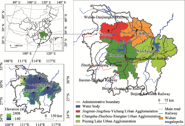
Figure 1 Location of the middle reaches of the Yangtze River urban agglomeration in China

3.2 Data sources and processing

For this study, land-use data for 2000, 2010, and 2020 were sourced from the Data Center for Resources and Environmental Sciences of the Chinese Academy of Sciences (http://www.resdc.cn), at resolution of 1000 × 1000 m. The overall accuracy has been assessed at > 90% (Liu et al., 2003; Liu et al., 2014; Ning et al., 2018). Land-use covers were divided into seven first class types—cultivated land, forestland, grassland, water area, wetland, construction land, and unused land—and 25 second class types. Traffic data for 2020 were supplemented by the National Geographic Information Center (NGCC) in 2017 (http://ngcc.sbsm.gov.cn/); whereas the traffic data for 2000 and 2010 were obtained by vectorization of the latest version of traffic data in 2000 and 2010 (Chen et al., 2019). A population distribution raster data with a 100 m resolution were sourced from WorldPop (https://www.worldpop.org/). Digital elevation models were adopted from the Geospatial Data Cloud, with a 90 meter resolution (http://www.gscloud.cn/).
In this study, a gridded evaluation unit was used to measure the coupling degree between the ESs S&D in the MRYRUA. To compare the possible influence of different grid unit sizes on the spatiotemporal pattern of ESs S&D, grid scales of 5 × 5 km and 10 × 10 km were selected as the basic units in this study based on previous research (Su et al., 2012; Li et al., 2016; Li et al., 2018; Zhang et al., 2018).

3.3 Methods

A semi-quantitative approach using ESs matrices proposed by Burkhard et al. (2009; 2012) was employed to quantify spatiotemporal patterns of ESs S&D. The Gini coefficient and the Lorenz curve were used for regional imbalances of ESs S&D (Gini, 1921). And the coupling degree of ESs S&D representing the degree of coordinated development between ESs supply and human demand was subsequently studied to reveal the level of the sustainability of regional ESs (Sun et al., 2019). The traffic accessibility in the MRYRUA was measured from the aspects of traffic density and traffic convenience based on multiple types of traffic data (Feng et al., 2009). The spatial relationships between traffic accessibility and the coupling degree of ESs S&D were ultimately evaluated using a series of spatial regression models (Chi, 2010; Chen et al., 2021) (Figure 2).
Figure 2 Framework of this study

3.3.1 Ecosystem services matrices

The ESs matrices proposed by Burkhard et al. (2009; 2012) were used to assign values to the biophysical units of ESs supply capacity and human demand through expert knowledge, thereby deriving a semi-quantitative measurement of ESs capability under land-use changes. In the ESs supply matrices, a score is given from 0 to 5 points, representing no, low, general, medium, high, and very high supply capacities, respectively. In the ESs demand matrices, a 0-5 score value is also set, representing no, low, general, medium, high, and very high demand capacities, respectively. This approach addresses the limitation that the dimensions of ESs S&D are difficult to unify due to the complexity of data acquisition. This method has been widely applied to study the S&D relationship of ESs in China (Li et al., 2016; Chen et al., 2020a).
Based on the studies of Costanza et al. (1997), de Groot et al. (2002), and the MA (2005), Burkhard et al. (2012) classified ESs into ecological integrity, regulating, supplying, and cultural services. Among them, the double counting of ESs involved in ecological integrity was considered (Wallace, 2007; Costanza, 2008; Burkhard et al., 2012), and is thus not included in the calculation processes of ESs matrices. In this study, S&D matrices of 19 ESs and 25 land-use types were constructed according to Burkhard et al. (2012). The ESs matrix method was employed in the following steps:
(1) Land-use data for 2000, 2010, and 2020 were classified according to the land use and land cover (LULC) classification system in “China’s 20th-century LULC space-time platform”, into 7 primary and 25 secondary land-use types (Liu et al., 2014; Ning et al., 2018); although notably, the classification system is significantly different from the land classification of coordinated information on the environment adopted in by Burkhard et al. (2009). The corresponding adjustment and merging of these two land types of classification systems were first conducted to determine the land classification system (Burkhard et al., 2009; Ou et al., 2018; Chen et al., 2020a).
(2) The current literature on ESs matrices in China was compiled and sorted, and values for each entry were assigned based on this research.
(3) The research team consulted 17 experts with different professional knowledge backgrounds in August 2019 in the study of Chen et al. (2020a). The experts included masters, doctoral students, and professors of land resource management, ecology, geography, rural sociology, regional economy, urban planning, and agricultural economics (Chen et al., 2020a).
(4) Questionnaires were used for expert consultation (N=17). According to different land-use types, the interviewed experts scored the importance of related ESs types independently, as well as the overall importance of each ESs in the MRYRUA. The final S&D matrix values of the ESs were ultimately determined by calculating the arithmetic mean values (Chen et al., 2020a).
(5) The obtained matrix values were assigned in batches to grid cells of 30 × 30 m using the vector calculation function of ArcGIS v.10.0. The matrix values and the corresponding land-use type area ratios were multiplied to obtain the relevant capacity values of the ESs supply index (ESSI), ESs demand index (ESDI), and ESs balance index (ESBI) in the study area.

3.3.2 Imbalance of ecosystem services

In this study, the Gini coefficients for each ESs supply, demand, and balance were calculated based on the characteristics of ESs supply and consumption to estimate their respective regional imbalances (Gini, 1921). The Gini coefficient of ESs supply consumption was used to measure the overall balance between regional ESs consumption and the ecological benefit acquisition under the same supply conditions.
The Gini coefficient is based on the Lorenz curve (Figure 3), which is commonly used in economics to analyze regional income disparity or wealth inequality (Gastwirth, 1971; 1972). In the Lorenz curve, the x-axis is the percentage of the population from the lowest to the highest income, and the y-axis is the cumulative share of income earned. The closer the Lorenz curve is to the 1:1 line, the more balanced is the income distribution. To more accurately understand this inequality, Gini (1921) proposed the Gini coefficient based on the Lorenz curve and the absolute fair line (Gini, 1921) referring to the proportion of the area enclosed by the line of equality and the Lorenz curve to the area between the line of equality and the absolute inequality line (OMN). In this, the area between the actual distribution curve and the absolute equity curve is referred to as S1, the area at the lower right of the actual income distribution curve is referred to as S2, and the Gini coefficient is equal to the ratio of S1: (S1+S2). When the Gini coefficient is over 0.4, the income gap is large, and when the Gini coefficient is over 0.5, the income gap is very evident. To distinctly reflect the spatial concentration and dispersion of ESSI, ESDI, and ESBI, this study employed both the Lorenz curve and the Gini coefficient to measure the balance of ESs S&D.
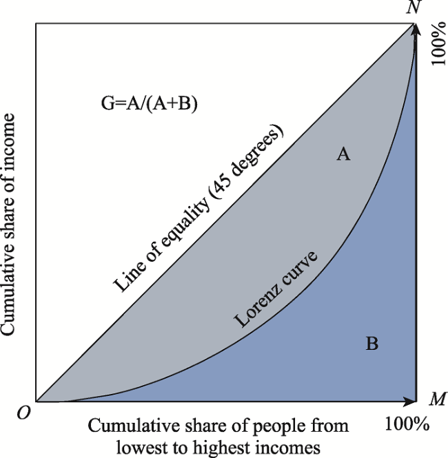
Figure 3 A typical Lorenz curve

3.3.3 Coupling degree of supply and demand of ecosystem services

The coupling degree of ESs S&D represents the degree of the coordinated development between ESs supply and human demand and reveals the level of the sustainability of regional ESs (Guan et al., 2019). The coupling degree was calculated according to Eq. (1):
$SDC{{D}_{it}}=\sqrt{\left[ \frac{ESS{{I}_{it}}\text{ }\!\!\times\!\!\text{ }ESD{{I}_{it}}}{{{\left( {\left( ESS{{I}_{it}}+ESD{{I}_{it}} \right)}/{2}\; \right)}^{2}}} \right]} $
where SDCDit represents the coupling degree between ESs S&D of the ith unit at time t, and ESSIit and ESDIit are the ESs S&D indices of the ith unit at time t, respectively.

3.3.4 Traffic accessibility

To represent the traffic accessibility of the MRYRUA, this study referred to the traffic accessibility calculation model constructed by Feng et al. (2009), combining the traffic data of railways, local and national highways, rivers, main hubs and general ports, as well as trunk and general airports. The traffic accessibility (TA) of the MRYRUA was measured from two aspects: traffic density (TD) and traffic convenience (TC) (Feng et al., 2009). Traffic density was used to represent the guaranteed degree of traffic facilities, and measured from three aspects: highway density (HD), railway density (RD), and navigable river density (NRD). Traffic convenience represents the connectivity degree with the outside world, and was measured via distances by road (RD), railway (RWD), urban center (UCD), airport (AD), and dock (DD). Each sub-index adopted the method of graded assignment, specific grade division and critical value (Zeng et al., 2018; Chen et al., 2021; Ge et al., 2021) according to Eqs. (2-4):
TA=(TD+TC)/2
TD=(HD+RD+NRD)/3
TC=(RD+RWD+UCD+AD+DD)/5

3.3.5 Spatial regression analysis

In this study, global bivariate spatial autocorrelation analysis was adopted to measure the spatial pattern between traffic accessibility and coupling degree of ESs S&D in the MRYRUA from a global perspective and the spatial distribution trend of measurement attribute values in the whole region (Anselin and Rey, 2014). To investigate the impact of traffic accessibility on the coupling degree of ESs S&D, a series of regression methods were used, including the least squares method (OLS), spatial lag model (SLM), spatial error model (SEM), and spatial error model with lag dependence (SEMLD) (Chi, 2010; Chen et al., 2021). The effects of traffic accessibility on the coupling degree of ESs S&D have been explored from multiple perspectives (Anselin and Rey, 2014). Specifically, the standard linear regression model assumes that the random error term of the model is independent and normally distributed, and the model diagnosis can be used to determine if the model hypothesis is satisfied. The OLS model comprehensively considers the importance of independent variables to dependent variables and does not consider the influence of neighborhood units. The SLM model assumes that spatial autocorrelation occurs in the dependent variables, emphasizes the neighborhood effect, and considers the spatial diffusion of the dependent variables among geographical units. The SEM model assumes that spatial autocorrelation exists in the disturbance error term and is used to measure the error impact of the dependent variables from adjacent geographical units on the observed values in the region. The spatial lag and spatial error models are too simplistic, which may exclude other possible spatial autocorrelation mechanisms, such as the coexistence of spatial autocorrelation between dependent variables and error terms. The SEMLD model, which includes the spatial lag and spatial error models, is a spatial autoregressive model enhanced by adding spatial lag dependent variables. The OLS, SEM, SLM, and SEMLD models were processed using Geoda 095i.

4 Results

4.1 Spatiotemporal distribution of ecosystem services supply, demand, and balance

Figures 4 and 5 show the spatiotemporal distribution of ESSI at 5 and 10 km grid scales in 2000, 2010, and 2020, respectively. The average ESSIs for the MRYRUA presented a decreasing trend: 56.266, 56.117, and 55.332 in 2000, 2010, and 2020, respectively. From a spatial perspective, it was found that the ESSI values in the plains—Jianghan Plain, Dongting Lake Plain, and Poyang Lake Plain—were significantly lower than that of the surrounding and central montane areas, indicating that the ESs supply capacity of the mountainous areas was greater than that of the plain areas. In addition, it was found that the supply capacity of ESs in the core areas of major traffic lines and cities was significantly lower than that of other areas.
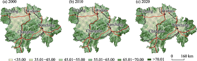
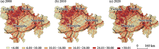
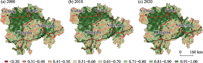
Figure 4 Spatial distribution of ESSI at 5 km grid scale in the middle reaches of the Yangtze River urban agglomeration
Figure 5 Spatial distribution of ESSI at 10 km grid scale in the middle reaches of the Yangtze River urban agglomeration
Figures 6 and 7 show the spatiotemporal distribution of the ESDI at the 5 and 10 km grid scales from 2000 to 2020, respectively. The average ESDIs continuously increased in the MRYRUA across the study period: 15.491, 15.705, and 16.250 in 2000, 2010, and 2020, respectively. In contrast to the spatial distribution of ESSI, the ESDI values were high and low in the plains and mountainous areas, respectively. The average ESBIs of the MRYRUA decreased across the study period: 40.775, 40.412, and 39.082 in 2000, 2010, and 2020, respectively. The spatial distribution was similar to that of the ESSI, lower in the plains than in the mountains.
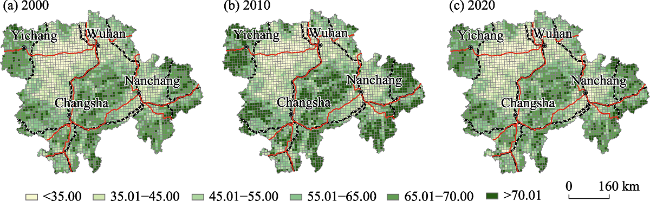
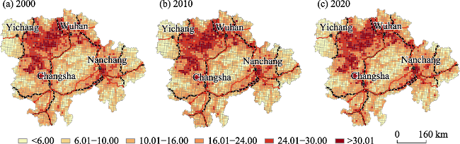
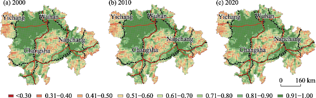
Figure 6 Spatial distribution of ESDI at 5 km grid scale in the middle reaches of the Yangtze River urban agglomeration
Figure 7 Spatial distribution of ESDI at 10 km grid scale in the middle reaches of the Yangtze River urban agglomeration

4.2 Change of ecosystem services balance

Based on the variables of the cumulative share of grid units, ESSI, ESDI, and ESBI, Lorenz curves for each ESs in the MRYRUA were plotted at 5 and 10 km grid scales from 2000 to 2020 (Figures 8-10). The Lorenz curves of the ESSI were closer to the line of equality, indicating a relatively spatially balanced distribution; however, the Lorenz curves of the ESDI varied heavily from the line of equality, indicating an uneven spatial distribution.
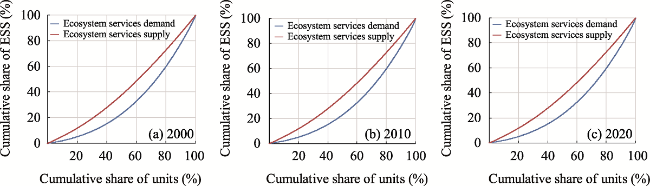
Figure 8 Lorenz curve of ecosystem services supply and demand in 2000, 2010, and 2020 at 5 km grid scale
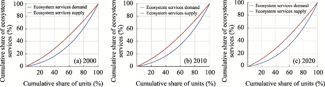
Figure 9 Lorenz curve of ecosystem services supply and demand in 2000, 2010, and 2020 at 10 km grid scale
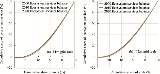
Figure 10 Lorenz curve of ecosystem services balance in 2000, 2010, and 2020 at 5 km and 10 km grid scales
The Gini coefficients at the 5 km scale ESSI were 0.162, 0.164, and 0.170 in 2000, 2010, and 2020, respectively; whereas those of the ESDI were 0.362, 0.366, and 0.371, respectively. At the 10 km scale, the Gini coefficients of ESSI were 0.150, 0.152, and 0.158; whereas those of ESDI were 0.338, 0.342, and 0.347, respectively. In general, the results showed that the ESSI and ESDI Gini coefficients at different scales did not exceed the warning value of 0.4, and the lowest Gini coefficient value of ESDI was markedly higher than that of ESSI. The increasing trend of the Gini coefficients across the entire time period indicated that the balance of the ESs supply was greater than that of the demand. For 2000, 2010, and 2020, the Gini coefficients for ESBI at a 5 km scale were 0.348, 0.356, and 0.381, respectively, and 0.319, 0.326, and 0.348, at a 10 km scale, respectively; thus, the Gini coefficient of ESBI showed an increasing trend at both scales, indicating an evident mismatch between the ESs S&D. In some regions, excessive consumption of ESs failed to generate an equivalent supply; moreover, this situation appears to be gradually worsening, with an increasing imbalance between supply and consumption of ESs in the region.

4.3 Spatiotemporal coupling degree of ecosystem services supply and demand

Figures 11 and 12 present the calculated coupling degree of ESs S&D at 5 and 10 km grid scales, respectively, for 2000 (0.823), 2010 (0.827), and 2020 (0.838). As the coupling degree of the ESs S&D in the MRYRUA was relatively higher and continuously increased, the sustainable capacity of regional ESs was high, and the relationship between ESs supply and human demand was in a comparatively balanced and sustainable state. In terms of spatial distribution, the coupling degree of the ESs S&D in the plains areas was significantly higher than that in the surrounding and central montane regions, which could be attributed to the plains being densely populated. Although rapid population growth and industrial development caused a rapid increase in supply consumption and caused a decline in the supply service capacity of the ecosystem, the development of the regional economy and society also created a rapid, non-linear growth of complex and diverse anthropogenic demands. With regard to spatial distribution, the characteristics of the SDCD were significantly correlated with terrain, traffic, and human activities.
Figure 11 Spatial distribution of SDCD at 5 km grid scale in the in the middle reaches of the Yangtze River urban agglomeration
Figure 12 Spatial distribution of SDCD at 10 km grid scale in the in the middle reaches of the Yangtze River urban agglomeration

4.4 Impact of traffic accessibility on coupling degree of ecosystem services supply and demand

Moran’s I analysis results of the MRYRUA in 2000, 2010, and 2020 showed that the bivariate spatial autocorrelation index between traffic accessibility and SDCD was 0.385, 0.381, and 0.382 at the 5 km scale and 0.429, 0.415, and 0.400 at the 10 km scale, respectively; all of them were significant at the p<0.0001 level. Bivariate Moran’s I analysis indicated that significant spatial dependence existed between traffic accessibility and SDCD. This implied that econometric models for spatial estimation and verification should be established. However, the selection of the optimum spatial regression model to best fit the data remains elusive. Commonly, a spatial dependence test is conducted to identify the appropriate model. The spatial lag model is more appropriate if: lagrange multiplier (LM) (log) is more statistically significant than LM (err), Robust LM (lag) is significant but Robust LM (err) is not, and the spatial error model is deemed to be the appropriate choice. If both are insignificant, the OLS model is more efficient. Additionally, log-likelihood (LogL), Akaike information criterion (AIC), and Schwartz criterion (SC) can be used to measure the model fitness, where the larger the LogL and the smaller the AIC and SC values, the better the model fit.
Following OLS estimation, the Moran’s I index residual test was performed. The Moran’s I coefficients of the residuals in 2000, 2010, and 2020 were 0.620, 0.626, and 0.601 at a 5 km scale and 0.621, 0.628, and 0.599 at a 10 km scale, respectively (Table 1). The p values at both scales were significant (< 0.0001), indicating strong spatial autocorrelation in the residuals. The spatial dependence diagnostics by the OLS model further documented that statistically significant spatial lag and spatial error terms existed in the model residuals (Table 1); thus, OLS estimation in previous classical linear regression models may have contained design errors without accounting for spatial autocorrelation. Considering the influences of the spatial lag and spatial error terms, the goodness of fit of the SLM, SEM, and SEMLD reasonably increased (Table 2). Robust LM (lag), Robust LM (error), and LM (lag and error) were all significant (p<0.0001), so SEM, SLM, and SEMLD models were deemed appropriate. Comparing the LogL, AIC, and SC values of the three spatial models, the SEMLD model maintained the largest LogL and smallest AIC and SC values, thereby indicating that it was the most robust. To accurately select the model, all these four regression model results are presented in Tables 1, 2, S1, and S2, where the superior fit of the spatial regression models over the OLS model can be observed.
Table 1 Regression results of the ordinary least squares (OLS)
Variable 5 km grid scale 10 km grid scale
2000 2010 2020 2000 2010 2020
Traffic accessibility 0.220***
(0.012)
0.220***
(0.012)
0.299***
(0.013)
0.206***
(0.019)
0.196***
(0.020)
0.270***
(0.020)
Population density 0.559***
(0.041)
0.550***
(0.044)
0.335***
(0.046)
0.580***
(0.062)
0.573***
(0.066)
0.406***
(0.068)
Elevation -0.929***
(0.017)
-0.934***
(0.011)
-0.939***
(0.010)
-0.816***
(0.017)
-0.833***
(0.017)
-0.844***
(0.017)
Constant 0.763***
(0.005)
0.759***
(0.005)
0.727***
(0.006)
0.752***
(0.009)
0.756***
(0.011)
0.726***
(0.011)
Moran’s I (error) 0.620*** 0.626*** 0.601*** 0.621*** 0.628*** 0.599***
LM (lag) 15238.516*** 15410.364*** 14136.079*** 3379.456*** 3415.517*** 3027.331***
Robust LM (lag) 36.419*** 21.949*** 25.780*** 12.996*** 5.576* 3.641
LM (error) 18445.007*** 18772.058*** 17334.164*** 4572.310*** 4655.374*** 4252.143***
Robust LM (error) 3242.909*** 3383.642*** 3223.865*** 1205.850*** 1255.433*** 1228.453***
LM (lag and error) 18481.425*** 18794.006*** 17359.944*** 4585.307*** 4670.950*** 4225.784***
Measures of fit
Log likelihood 6150.210 6092.970 6189.220 2090.020 2048.960 2074.740
AIC -12292.400 -12177.900 -12370.400 -4172.040 -4089.920 -4141.470
SC -12262.600 -12148.100 -12340.600 -4147.640 -4065.520 -4117.070
R-squared 0.501 0.498 0.507 0.576 0.568 0.581
N 12712 12712 12712 3299 3299 3299

Note: The study uses the queen’s contiguity weight matrix. ***p≤0.001, *p≤0.05. Standard errors are in parentheses. LM = Lagrange multiplier. AIC = Akaike information criterion. SC = Schwarz criterion.

Table 2 Regression results of the spatial error models with lag dependence in 2000, 2010, and 2020
Variable 5 km grid scale 10 km grid scale
2000 2010 2020 2000 2010 2020
Traffic accessibility 0.031***
(0.006)
0.036***
(0.006)
0.037***
(0.007)
0.047***
(0.011)
0.050***
(0.012)
0.074***
(0.013)
Population density 0.102***
(0.021)
0.098***(0.023) 0.047*
(0.024)
0.231***
(0.038)
0.215***
(0.041)
0.152***
(0.043)
Elevation -0.049***
(0.006)
-0.048***
(0.006)
-0.052***
(0.006)
-0.114***
(0.012)
-0.109***
(0.013)
-0.126***
(0.013)
Spatial lag term -0.475***
(0.019)
-0.465***
(0.019)
-0.470***
(0.019)
-0.278***
(0.035)
-0.294***
(0.036)
-0.264***
(0.035)
Spatial error term 0.999***
(0.005)
0.999***
(0.005)
1.000***
(0.005)
0.935***
(0.011)
0.943***
(0.011)
0.929***
(0.011)
Constant -0.007
(0.004)
-0.010*
(0.004)
-0.011*
(0.005)
0.036***
(0.010)
0.028**
(0.010)
0.029**
(0.037)
Log likelihood 11999.890 11988.570 11707.046 3448.866 3415.243 3310.822
AIC -23989.800 -23967.100 -23404.100 -6887.730 -6820.490 -6611.640
SC -23952.500 -23929.900 -23366.800 -6857.22 -6789.980 -6581.140
R2 0.807 0.807 0.799 0.816 0.814 0.804
N 12712 12712 12712 3299 3299 3299

Note: The study uses the queen’s contiguity weight matrix. ***p≤0.001, **p≤0.01, *p≤0.05. Standard errors are in parentheses. AIC = Akaike information criterion. SC = Schwarz criterion.

Using SEMLD for interpretation, a 10% increase in traffic accessibility would correlate to a 0.310%, 0.360%, and 0.370% increase in SDCD at the 5 km scale, and a 10% increase in traffic accessibility would correlate to a 0.47%, 0.500%, and 0.74% increase in SDCD at the 10 km level in 2000, 2010, and 2020. The regression coefficients at the 5 km grid scale were lower than those at the 10 km, and an increasing tendency was also observed in the regression coefficients of traffic accessibility on SDCD, indicating that its influence on SDCD is increasing. Furthermore, an increase in population density is projected to lead to an increase in SDCD, while increasing elevation would lead to a decrease.

5 Discussion and implications

5.1 Driving mechanism of traffic accessibility on the coupling degree of ES ecosystem services supply and demand

Flow, supply, and demand are the three basic links of ESs. The movement of ESs from one region to another for anthropogenic use forms ESs flow (Burkhard et al., 2014; Baró et al., 2016; Wang et al., 2021). Based on the spatial relationship of ESs delivery, ESs flows aregenerally divided into three categories: in-situ services, omnidirectional services, and directional services (Fisher et al., 2009). ESs flow should rely on a carrier, under the influence of natural or human factors, along a certain direction or path towards anthropogenic use areas (Fisher et al., 2009). The flow of most ESs (e.g., supplying services) inherently relies on some carriers or tools (Johnson et al., 2012); however, some ESs flows may not require a carrier, as they are a service in themselves (e.g., water). There is a further special kind of ESs flow that is realized by public’s active movement to service supply areas, such as cultural services. The carrier of ESs flow can be a biological factor or abiotic factor and can assist with the delivery of services as a carrier mechanism or directly provide the service itself (e.g., water, air, animals, and transportation) (Johnson et al., 2012; Liu et al., 2017). As an important carrier, traffic can connect the ESs S&D, thereby affecting the strength of their coupling.
Traffic is not only an important carrier of ESs flow, but also affects ESs balance by affecting ESs supply capacity and ESs demand capacity (Chen et al., 2020a; Chen et al., 2021). Previous studies have shown that the improvement of traffic accessibility reduces the supply capacity and increases the demand capacity of ESs (Chen et al., 2020a; Chen et al., 2021). The improvement of traffic conditions can promote the agglomeration of various production factors and the development of the local economy, thus reshaping the regional spatial structure (Voss and Chi, 2006; Chi, 2010; Wang et al., 2019; Ge et al., 2021). For example, the increase in traffic accessibility can exacerbate landscape fragmentation, thereby detrimentally affecting the supply capacity of the ecosystem (Spellerberg, 1998; Liu et al., 2019; Wei et al., 2020). In addition, traffic accessibility can promote the flow of population, economic development, and expansion of construction land and thus increase the demand capacity of ESs (Chi, 2010; Tan et al., 2014; Wang et al., 2019).
Traffic accessibility is reflective of anthropogenic activity intensity and urban development (Ge et al., 2021). Economic progress has also brought about the development of traffic accessibility processes that do not play a direct role in the increase of SDCD, but promote an increase in urban construction, population growth, and infrastructure construction, thereby indirectly increasing ESs demand (Tan et al., 2014; Wang et al., 2019; Chen et al., 2020a; Wu et al., 2020).
In this study, we analyzed not only the correlations between traffic accessibility and SDCD from 2000 to 2020 at both the 5 km grid and 10 km grid scales, but also the population density and elevation. According to the results, population density is positively correlated with SDCD, while elevation is negatively correlated with SDCD. In previous studies, Xu et al. (2021) suggested that the high levels of economic development, population density, and increasing demand for construction land in the city center led to increased ESs demand and weakened supply capacity. Sun et al. (2020) analyzed spatiotemporal changes in ESs S&D across the conterminous United States. They concluded that ESs supply was mainly affected by population density, road density, per capita GDP by industry, patch density, average annual precipitation, and per capita energy consumption. ESs demand was mainly affected by population density, road density, mean elevation, per capita income, per capita GDP by industry, average annual precipitation, and per capita water use per day. Some studies also explored the relationship between ESs S&D and urbanization (Cao et al., 2021; Pan and Wang, 2021; Shi et al., 2021)

5.2 Scale effects between traffic accessibility and the coupling degree of ecosystem services

Different ESs arise through combinations of social-ecological drivers and interact with each other across scales. It is essential to design effective policy interventions toward achieving sustainability by clarifying the relationships among ESs and the underlying drivers at different scales (Shen et al., 2021). Many scholars carried out empirical research on the assessment of ESs S&D at a specific spatial scale (Baró et al., 2015; Sahle et al., 2017). To date, there are only a few reports concerning the analysis of ESs mismatch at multiple scales and integrated spatiotemporal dimensions (Sun et al., 2019). Thus, it is important to fully understand the spatial relationships between traffic accessibility and ESs S&D across multiple spatiotemporal scales.
In this study, we not only analyzed the changes in traffic accessibility and ESs S&D from 2000 to 2020 at both 5 km grid and 10 km grid scales, but also analyzed the scale effects on the spatial relationships between traffic accessibility and coupling degree of ESs S&D. The spatial distribution of ESSI and ESDI exhibited similarities at the two scales of analysis. As the scale became coarser, the spatial clustering of high ESSI, high SDCD, and low ESDI values appeared to be more obvious in the mountainous areas. Moreover, the Gini coefficients for ESBI at the 5 km scale were higher than that at the 10 km scale, indicating an evident mismatch between the ESs S&D at the 5 km scale. Using SEMLD for interpretation, we found that a 10% increase in traffic accessibility would respectively correlate to higher increase in SDCD at the 10 km scale than at the 5 km level in 2000, 2010, and 2020.

5.3 Policy implications

ESs are transferred from natural to socioeconomic systems for anthropogenic use, forming the flow of ESs in an effort to meet the demand for the consumption and use of these products and services. Research on the coupling degree between ESs S&D can reveal the evolution characteristics of the human-land relationship, and reflect whether they are harmonious and constant (Guan et al., 2019; Xie et al., 2020). The results showed that the coupling degree between ESs S&D in the MRYRUA increased over the study period from 2000 to 2020, indicating that the sustainability of ESs increased continuously. In addition, the coupling degree of ESs S&D in mountainous regions of the MRYRUA was much lower than that of the plain areas, with the surplus areas of ESs primarily distributed in the former, and deficit areas in the latter (Lorilla et al., 2019).
Due to large populations, frequent human activity, high intensity of land use, and urbanization of the plains areas, the supply of ESs may not be able to meet the entirety of anthropogenic needs, and the coupling degree of ESs S&D would be unbalanced for the foreseeable future (Ge et al., 2021; Zhang et al., 2021). Different strategies for S&D management of ESs should be adopted for each region to achieve an optimal balance. For example, we should take measures to improve urban green infrastructure and corridor landscapes in urban areas, as with parks and leisure green spaces, vegetation coverage, in an effort to comprehensively balance ESs and economic development (Dai et al., 2021). Traffic accessibility can impact ESs S&D by affecting land use change, thus altering the supply capacity of ESs (Spellerberg, 1998; Liu et al., 2019; Chen et al., 2021). Therefore, optimizing the land-use structure and enhancing regional land-intensive and economic utilization of regions is of great significance. Simultaneously, traffic accessibility can lead to increased ESs demand, playing an important role in the process of connecting the ESs S&D. As traffic accessibility would remain an important factor affecting the coupling of ESs S&D in the future, the MRYRUA needs to improve the traffic network, break through the “dead-end road,” build a network-like multi-nodal regional traffic system, and improve the functionality of ESs flow carriers. In addition, the construction of road green space should be strengthened, and the road green space should be managed under an ecological agriculture model (Zhang et al., 2017). In the future urban transportation construction, theory of ecological transportation must be developed. According to the principles of natural ecology, economic ecology and human ecology, an ecological traffic system composed of traffic networks, vehicles, and traffic environment for planning, construction and management can be developed (Chen and Ou, 2019). In addition, the department should strengthen overall planning, and incorporate ecological benefits into traffic planning.

5.4 Limitations and future directions

Based on the ESs matrix method, this study measured the coupling degree between grid-scale ESs S&D for the MRYRUA. Spatial regression approaches were used to measure the impact of traffic accessibility on the degree of ESs S&D coupling. When including expert knowledge, it is difficult to avoid subjectivity, and therefore, biophysical data can be incorporated in future studies (Sun et al., 2020; Cao et al., 2021). In the present study, regional scale spatial regression models were used to analyze the influence of traffic accessibility on the SDCD; however, the exploration of local features was lacking, necessitating future research. Furthermore, the coupling between ESs S&D was measured based on 5 and 10 km grid scales, we can find evident differences in the impacts of traffic accessibility on the degree of coupling at different spatiotemporal scales. Thus variable spatiotemporal scales should also be considered in future analyses to help elucidate any pertinent patterns.

6 Conclusions

In this study, the spatiotemporal characteristics of ESs S&D in the MRYRUA were measured using the ESs matrix method, and the relationship between them was analyzed based on their coupling degree. A series of spatial regression models were then used to analyze the influence of traffic accessibility on the coupling degree of ESs. The results showed that the ESSI, ESDI, and ESBI in the MRYRUA continuously decreased, while the ESDI continuously increased from 2000 to 2020. The S&D index of ESs and the Gini coefficient of the balance index continuously increased without exceeding the warning value of 0.4. The coupling degree of ESs S&D also continuously increased, and the spatial distribution characteristics were similar to that of the ESDI, exhibiting significantly higher values in the plains than the montane regions, which was contrary to the observed patterns of the ESSI. The results of the global bivariate Moran’s I analysis showed that there was a significant spatial dependence between traffic accessibility and ESs S&D. The results of spatial regression showed that an increase in traffic accessibility would promote the coupling degree of ESs S&D, thereby supporting that improved traffic accessibility could promote the circulation of ESs.
Table S1 Regression results of the spatial lag model (SLM) and spatial error model (SEM) at 5k m grid scale in 2000, 2010, and 2020
Variable 2000 2010 2020
SLM SEM SLM SEM SLM SEM
Traffic accessibility 0.079***
(0.008)
0.111***(0.010) 0.084***
(0.008)
0.123***
(0.010)
0.104***
(0.009)
0.132***
(0.012)
Population density 0.217***
(0.027)
0.283***(0.034) 0.213***
(0.029)
0.298**(0.038) 0.130***
(0.031)
0.224***
(0.041)
Elevation -0.256***
(0.010)
-0.939***
(0.018)
-0.254***
(0.010)
-0.940***
(0.019)
-0.271***
(0.010)
-0.969***
(0.019)
Spatial lag term 0.792***
(0.007)
0.794***
(0.006)
0.782***
(0.007)
Spatial error term 0.853***(0.006) 0.855***
(0.006)
0.847***
(0.006)
Constant 0.152***
(0.006)
0.802***(0.007) 0.146***(0.06) 0.796***
(0.007)
0.148***
(0.006)
0.798***
(0.008)
Measures of fit
Log likelihood 10815.800 11348.963 10805.500 11361.028 10555.500 11093.583
AIC -21621.600 -22689.900 -21601.100 -22714.100 -21101.000 -22179.200
SC -21584.400 -22660.100 -21563.800 -22684.300 -21063.800 -22149.400
R2 0.788 0.811 0.788 0.743 0.780 0.804
N 12712 12712 12712 12712 12712 12712

Note: The study uses the queen’s contiguity weight matrix. ***p≤0.001, **p≤0.01. Standard errors are in parentheses. AIC = Akaike information criterion. SC = Schwarz criterion.

Table S2 Regression results of the spatial lag model (SLM) and spatial error model (SEM) at 10 km grid scale in 2000, 2010, and 2020
Variable 2000 2010 2020
SLM SEM SLM SEM SLM SEM
Traffic accessibility 0.086***
(0.013)
0.124***
(0.015)
0.088***
(0.014)
0.141***
(0.016)
0.124***
(0.014)
0.172***
(0.017)
Population density 0.310***
(0.042)
0.304***
(0.044)
0.287***
(0.044)
0.279**
(0.048)
0.212***
(0.048)
0.218***
(0.051)
Elevation -0.273***
(0.017)
-0.849***
(0.025)
-0.277***
(0.017)
-0.859***
(0.025)
-0.297***
(0.017)
-0.879***
(0.026)
Spatial lag term 0.749***
(0.013)
0.752***
(0.013)
0.732***
(0.014)
Spatial error term 0.857***
(0.011)
0.857***
(0.011)
0.842***
(0.012)
Constant 0.178***
(0.012)
0.792***
(0.012)
0.174***
(0.012)
0.785***
(0.013)
0.174***
(0.012)
0.774***
(0.013)
Measures of fit
Log likelihood 3219.170 3467.230 3180.950 3436.602 3093.230 3332.365
AIC -6428.340 -6926.460 -6351.900 -6865.200 -6176.450 -6656.730
SC -6397.840 -6902.050 -6321.400 -6840.800 -6145.950 -6632.320
R2 0.808 0.843 0.805 0.841 0.796 0.832
N 3299 3299 3299 3299 3299 3299

Note: The study uses the queen’s contiguity weight matrix. ***p≤0.001, **p≤0.01. Standard errors are in parentheses. LM = Lagrange multiplier. AIC = Akaike information criterion. SC = Schwarz criterion.

[1]
Anselin L, Rey S J, 2014. Modern spatial econometrics in practice:A guide to GeoDa. GeoDa Press LLC, GeoDaSpace and PySAL.

[2]
Bagstad K J, Johnson G W, Voigt B, et al., 2013. Spatial dynamics of ecosystem service flows: A comprehensive approach to quantifying actual services. Ecosystem Services, 4: 117-125.

DOI

[3]
Baró F, Haase D, Gómez-Baggethun E, et al., 2015. Mismatches between ecosystem services supply and demand in urban areas: A quantitative assessment in five European cities. Ecological Indicators, 55: 146-158.

DOI

[4]
Baró F, Palomo I, Zulian G, et al., 2016. Mapping ecosystem service capacity, flow, and demand for landscape and urban planning: A case study in the Barcelona metropolitan region. Land Use Policy, 57: 405-417.

DOI

[5]
Brauman K A, Daily G C, Duarte T K, et al., 2007. The nature and value of ecosystem services: an overview highlighting hydrologic services. Annual Review of Environment and Resources, 32: 67-98.

[6]
Burkhard B, Kandziora M, Hou Y, et al., 2014. Ecosystem service potentials flow and demands: Concepts for spatial localization, indication, and quantification. Landscape Online, 34: 1-32.

DOI

[7]
Burkhard B, Kroll F, Müller F, 2009. Landscapes capacities to provide ecosystem services: A concept for land-cover-based assessments. Landscape Online, 15: 1-22.

DOI

[8]
Burkhard B, Kroll F, Nedkov S, et al., 2012. Mapping ecosystem service supply, demand and budgets. Ecological Indicators, 21: 17-29.

DOI

[9]
Cao T, Yi Y, Liu H, et al., 2021. The relationship between ecosystem service supply and demand in plain areas undergoing urbanization: A case study of China’s Baiyangdian Basin. Journal of Environmental Management, 289: 112492.

DOI

[10]
Chen W, Chi G, Li J, 2020a. The spatial aspect of ecosystem services balance and its determinants. Land Use Policy, 90: 104263.

DOI

[11]
Chen W, Chi G, Li J, 2020b. Ecosystem services and their driving forces in the middle reaches of the Yangtze River urban agglomerations, China. International Journal of Environmental Research and Public Health, 17: 3717.

DOI

[12]
Chen W, Li J, Xiong J, et al., 2018. Differences in driving-force mechanisms in urban land expansion in China based on GWR. Journal of Henan University (Natural Science), 48(5): 522-530. (in Chinese)

[13]
Chen W, Li J, Zeng J, et al., 2019. Spatial heterogeneity and formation mechanism of eco-environmental effect of land use change in China. Geographical Research, 38(9): 2173-2187. (in Chinese)

DOI

[14]
Chen W, Ou L, 2019. The theory of ecological transportation and regional ecological traffic condition evaluation: Taking Beijing as an example. Ecological Economy, 35: 94-99. (in Chinese)

[15]
Chen W, Zeng Y, Zeng J, 2021. Impacts of traffic accessibility on ecosystem services: An integrated spatial approach. Journal of Geographical Sciences, 31(12): 1816-1836.

DOI

[16]
Chi G, 2010. The impacts of highway expansion on population change: An integrated spatial approach. Rural Sociology, 75: 58-89.

DOI

[17]
Costanza R, 2008. Ecosystem services: Multiple classification systems are needed. Biological Conservation, 141: 350-352.

DOI

[18]
Costanza R, DArge R, DeGroot R, et al., 1997. The value of the world’s ecosystem services and natural capital. Nature, 387: 253-260.

DOI

[19]
Cui X, Fang C, Liu H, et al., 2019. Dynamic simulation of urbanization and eco-environment coupling: A review on theory, methods, and applications. Acta Geographica Sinica, 74(6): 1079-1096. (in Chinese)

[20]
Dai X, Wang L, Tao M, et al., 2021. Assessing the ecological balance between supply and demand of blue-green infrastructure. Journal of Environmental Management, 288: 112454.

DOI

[21]
De Groot R S, Wilson M A, Boumans R M J, 2002. A typology for the classification, description, and valuation of ecosystem functions, goods, and services. Ecological Economics, 41: 393-408.

DOI

[22]
Fang C, Wang Z, Ma H, 2018. The theoretical cognition of the development law of China’s urban agglomeration and academic contribution. Acta Geographica Sinica, 73(4): 651-665. (in Chinese)

[23]
Fang C, Yu D, 2017. Urban agglomeration: An evolving concept of an emerging phenomenon. Landscape and Urban Planning, 162: 126-136.

DOI

[24]
Feng Z, Liu D, Yang Y, 2009. Evaluation of transportation ability of China: From county to province level. Geographical Research, 28(2): 419-429. (in Chinese)

DOI

[25]
Feurer M, Rueff H, Celio E, et al., 2021. Regional scale mapping of ecosystem services supply, demand, flow and mismatches in Southern Myanmar. Ecosystem Services, 52: 101363.

DOI

[26]
Fisher B, Turner R K, 2008. Ecosystem services: Classification for valuation. Biological Conservation, 141: 1167-1169.

DOI

[27]
Fisher B, Turner R K, Morling P, 2009. Defining and classifying ecosystem services for decision making. Ecological Economics, 68: 643-653.

DOI

[28]
Gastwirth J L, 1971. A general definition of the Lorenz Curve. Econometrica, 39: 1037-1039.

DOI

[29]
Gastwirth J L, 1972. The estimation of the Lorenz Curve and Gini Index. The Review of Economics and Statistics, 54: 306-316.

DOI

[30]
Ge F, Chen W, Zeng Y, et al., 2021. The nexus between urbanization and traffic accessibility in the middle reaches of the Yangtze River urban agglomerations, China. International Journal of Environmental Research and Public Health, 18: 3828.

DOI

[31]
Gini C. 1921. Measurement of inequality of incomes. The Economic Journal, 31(121): 124-125.

DOI

[32]
González-García A, Palomo I, González J A, et al., 2020. Quantifying spatial supply-demand mismatches in ecosystem services provides insights for land-use planning. Land Use Policy, 94: 104493.

DOI

[33]
Guan Q, Hao J, Xu Y, et al., 2019. Zoning of agroecological management based on the relationship between supply and demand of ecosystem services. Resources Science, 41(7): 1359-1373. (in Chinese)

DOI

[34]
Guida-Johnson B, Zuleta G A, 2013. Land-use land-cover change and ecosystem loss in the Espinal ecoregion, Argentina. Agriculture, Ecosystems & Environment, 181: 31-40.

DOI

[35]
Gulyás A, Kovács Á, 2016. Assessment of transport connections based on accessibility. Transportation Research Procedia, 14: 1723-1732.

DOI

[36]
Gutiérrez J L, 2001. Location, economic potential and daily accessibility: An analysis of the accessibility impact of the high-speed line Madrid-Barcelona French border. Journal of Transport Geography, 9: 229-242.

DOI

[37]
Hansen W G, 1959. How accessibility shapes land use. Journal of the American Institute of Planners, 25(2): 73-76.

DOI

[38]
Hu X W, Su Y Q, Ren K F, et al., 2021. Measurement and influencing factors of urban traffic ecological resilience in developing countries: A case study of 31 Chinese cities. Regional Sustainability, 2(3): 211-223.

DOI

[39]
Jin F, Chen Z, 2019. Evolution of transportation in China since reform and opening-up: Patterns and principles. Acta Geographica Sinica, 74(10): 1941-1961. (in Chinese)

DOI

[40]
Jing Y, Chen L, Sun R, 2018. A theoretical research framework for ecological security pattern construction based on ecosystem services supply and demand. Acta Ecologica Sinica, 38(12): 4121-4131. (in Chinese)

[41]
Johnson G W, Bagstad K J, Snapp R R, et al., 2012. Service path attribution networks (SPANs): A network flow approach to ecosystem service assessment. International Journal of Agricultural and Environmental, 3: 54-71.

[42]
Li B, Chen N, Wang Y, et al., 2018. Spatiotemporal quantification of the trade-offs and synergies among ecosystem services based on grid-cells: A case study of Guanzhong Basin, NW China. Ecological Indicators, 94: 246-253.

DOI

[43]
Li J, Jiang H, Bai Y, et al., 2016. Indicators for spatial-temporal comparisons of ecosystem service status between regions: A case study of the Taihu River Basin, China. Ecological Indicators, 60: 1008-1016.

DOI

[44]
Liu H, Liu L, Ren J, et al., 2017. Progress of quantitative analysis of ecosystem service flow. Chinese Journal of Applied Ecology, 28(8): 2723-2730. (in Chinese)

[45]
Liu J, Kuang W, Zhang Z, et al., 2014. Spatiotemporal characteristics, patterns, and causes of land-use changes in China since the late 1980s. Journal of Geographical Sciences, 24(2): 195-210.

DOI

[46]
Liu J, Liu M, Zhuang D, et al., 2003. Study on the spatial pattern of land-use change in China during 1995-2000. Science in China Series D: Earth Sciences, 46(4): 373-384.

[47]
Liu W, Zhan J, Zhao F, et al., 2022. The tradeoffs between food supply and demand from the perspective of ecosystem service flows: A case study in the Pearl River Delta, China. Journal of Environmental Management, 301: 113814.

DOI

[48]
Liu Y, Cao X, Xu J, et al., 2019. Influence of traffic accessibility on land use based on Landsat imagery and internet map: A case study of the Pearl River Delta urban agglomeration. Plos One, 14: e224136.

[49]
Lorilla R S, Kalogirou S, Poirazidis K, et al., 2019. Identifying spatial mismatches between the supply and demand of ecosystem services to achieve a sustainable management regime in the Ionian Islands (Western Greece). Land Use Policy, 88: 104171.

[50]
Mehring M, Ott E, Hummel D, 2018. Ecosystem services supply and demand assessment: Why social-ecological dynamics matter. Ecosystem Services, 30: 124-125.

DOI

[51]
Meng Q, Yang H, 2002. Benefit distribution and equity in road network design. Transportation Research Part B: Methodological, 36(1): 345-363.

DOI

[52]
Mononen L, Auvinen A P, Ahokumpu A L, et al., 2016. National ecosystem service indicators: Measures of social-ecological sustainability. Ecological Indicators, 61(1): 27-37.

DOI

[53]
Ning J, Liu J, Kuang W, et al., 2018. Spatiotemporal patterns and characteristics of land-use change in China during 2010-2015. Journal of Geographical Sciences, 28(5): 547-562.

DOI

[54]
Ou W, Wang H, Tao Y, 2018. A land cover-based assessment of ecosystem services supply and demand dynamics in the Yangtze River Delta region. Acta Ecologica Sinica, 38(17): 6337-6347. (in Chinese)

[55]
Pan Z, Wang J, 2021. Spatially heterogeneity response of ecosystem services supply and demand to urbanization in China. Ecological Engineering, 169: 106303.

DOI

[56]
Millennium Ecosystem Assessment (MA), 2005. Ecosystems and Human Well-being. Washington, DC: Island Press.

[57]
Sahle M, Saito O, Furst C, et al., 2017. Quantification and mapping of the supply of and demand for carbon storage and sequestration service in woody biomass and soil to mitigate climate change in the socio-ecological environment. Science of The Total Environment, 624: 342-354.

DOI

[58]
Shen J, Li S, Liu L, et al., 2021. Uncovering the relationships between ecosystem services and social-ecological drivers at different spatial scales in the Beijing-Tianjin-Hebei region. Journal of Cleaner Production, 290: 125193.

DOI

[59]
Shi Y, Feng C, Yu Q, et al., 2021. Integrating supply and demand factors for estimating ecosystem services scarcity value and its response to urbanization in typical mountainous and hilly regions of south China. Science of The Total Environment, 796: 149032.

DOI

[60]
Spake R, Lasseur R, Crouzat E, et al., 2017. Unpacking ecosystem service bundles: Towards predictive mapping of synergies and trade-offs between ecosystem services. Global Environmental Change, 47: 37-50.

DOI

[61]
Spellerberg I, 1998. Ecological effects of roads and traffic: A literature review. Global Ecology & Biogeography, 7: 317-333.

[62]
Su S, Xiao R, Zhang Y, 2012. Multi-scale analysis of spatially varying relationships between agricultural landscape patterns and urbanization using geographically weighted regression. Applied Geography, 32(2): 360-375.

DOI

[63]
Sun W, Li D, Wang X, et al., 2019. Exploring the scale effects, trade-offs and driving forces of the mismatch of ecosystem services. Ecological Indicators, 103: 617-629.

DOI

[64]
Sun X, Tang H, Yang P, et al., 2020. Spatiotemporal patterns and drivers of ecosystem service supply and demand across the conterminous United States: A multiscale analysis. Science of The Total Environment, 703: 135005.

DOI

[65]
Tan R, Liu Y, Liu Y, et al., 2014. Urban growth and its determinants across the Wuhan urban agglomeration, central China. Habitat International, 44: 268-281.

DOI

[66]
Tan Z, Li S, Li X, et al., 2017. Spatio-temporal effects of urban rail transit on complex land-use change. Acta Geographica Sinica, 72(5): 850-862. (in Chinese)

DOI

[67]
Tao Y, Wang H, Ou W, et al., 2018. A land-cover-based approach to assessing ecosystem services supply and demand dynamics in the rapidly urbanizing Yangtze River Delta region. Land Use Policy, 72: 250-258.

DOI

[68]
Voss P R, Chi G Q, 2006. Highways and population change. Rural Sociology, 71(1): 33-58.

DOI

[69]
Wallace K J, 2007. Classification of ecosystem services: Problems and solutions. Biological Conservation, 139(3/4): 235-246.

DOI

[70]
Wang C, Li W, Sun M, et al., 2021. Exploring the formulation of environmental management policies by quantifying interregional primary ecosystem service flows in Yangtze River Delta region, China. Journal of Environmental Management, 284: 112042.

DOI

[71]
Wang F, Wei X, Liu J, et al., 2019. Impact of high-speed rail on population mobility and urbanization: A case study on Yangtze River Delta urban agglomeration, China. Transportation Research Part A: Policy and Practice, 127: 99-114.

[72]
Wang J, Zhai T, Lin Y, et al., 2019. Spatial imbalance and changes in supply and demand of ecosystem services in China. Science of the Total Environment, 657: 781-791.

DOI

[73]
Wei L, Luo Y, Wang M, et al., 2020. Essential fragmentation metrics for agricultural policies: Linking landscape pattern, ecosystem service, and land use management in urbanizing China. Agricultural Systems, 182: 102833.

DOI

[74]
Wu C, Huang X, Chen B, 2020. Telecoupling mechanism of urban land expansion based on transportation accessibility: A case study of transitional Yangtze River economic Belt, China. Land Use Policy, 96: 104687.

DOI

[75]
Xie X, Zhang S, Lin B, et al., 2020. Spatial zoning for land ecological consolidation in Guangxi based on the ecosystem services supply and demand. Journal of Natural Resources, 35(1): 217-229. (in Chinese)

DOI

[76]
Xu Q, Yang R, Zhuang D, et al., 2021. Spatial gradient differences of ecosystem services supply and demand in the Pearl River Delta region. Journal of Cleaner Production, 279: 123849.

DOI

[77]
Xu Z, Peng J, Dong J, et al., 2022. Spatial correlation between the changes of ecosystem service supply and demand: An ecological zoning approach. Landscape and Urban Planning, 217: 104258.

DOI

[78]
Yang R, 2017. An analysis of rural settlement patterns and their effect mechanisms based on road traffic accessibility of Guangdong. Acta Geographica Sinica, 72(10): 1859-1871. (in Chinese)

DOI

[79]
Yu H, Xie W, Sun L, et al., 2021. Identifying the regional disparities of ecosystem services from a supply-demand perspective. Resources, Conservation and Recycling, 169: 105557.

[80]
Zeng Y, Hu S, Qu S, 2018. Spatial-temporal coupling of traffic location change and construction land expansion in the middle of Yangtze River Economic Belt. Resources and Environment in the Yangtze Basin, 27(12): 2651-2662. (in Chinese)

[81]
Zhang C, Sun J, Wang W, et al., 2017. Ecosystem service values and ecological costs of urban road green space in Yongjia county under different management models. Resources Science, 39(3): 522-532. (in Chinese)

[82]
Zhang G, Zheng D, Xie L, et al., 2021. Mapping changes in the value of ecosystem services in the Yangtze River Middle Reaches Megalopolis, China. Ecosystem Services, 48: 101252.

DOI

[83]
Zhang Y, Li X, Min Q, 2019. Transportation accessibility of central towns in important agricultural heritage systems sites in mountainous areas and its impact on local economic development: A case study of Honghe Hani Rice Terraced System, Yunnan. Journal of Resources and Ecology, 10(1): 29-38.

DOI

[84]
Zhang Y, Liu Y, Zhang Y, et al., 2018. On the spatial relationship between ecosystem services and urbanization: A case study in Wuhan, China. Science of the Total Environment, 637: 780-790.

[85]
Zhu X, Zhang P, Wei Y, et al., 2019. Measuring the efficiency and driving factors of urban land use based on the DEA method and the PLS-SEM model: A case study of 35 large and medium-sized cities in China. Sustainable Cities and Society, 50: 101646,

DOI

[86]
Zondag B, Bok M D, Geurs K T, et al., 2015. Accessibility modeling and evaluation: The TIGRIS XL land-use and transport interaction model for the Netherlands. Computers, Environment and Urban Systems, 49: 115-125.

DOI

Outlines

/