Research Articles

Influencing factors of manufacturing agglomeration in the Beijing-Tianjin-Hebei region based on enterprise big data

  • HUANG Yujin , 1, 2 ,
  • SHENG Kerong 3 ,
  • SUN Wei , 1, 2, *
Expand
  • 1.Institute of Geographic Sciences and Natural Resources Research, CAS, Beijing 100101, China
  • 2.College of Resources and Environment, University of Chinese Academy of Sciences, Beijing 100049, China
  • 3.School of Economics, Shandong University of Technology, Zibo 255012, Shandong, China
* Sun Wei (1975-), PhD and a professor at the University of Chinese Academy of Sciences, specialized in economic geography and regional development. E-mail:

Huang Yujin, PhD Candidate, specialized in economic geography. E-mail:

Received date: 2022-05-08

  Accepted date: 2022-07-12

  Online published: 2022-12-25

Supported by

Strategic Priority Research Program of the Chinese Academy of Sciences(XDA19040401)

National Natural Science Foundation of China(41871117)

National Natural Science Foundation of China(41771173)

Abstract

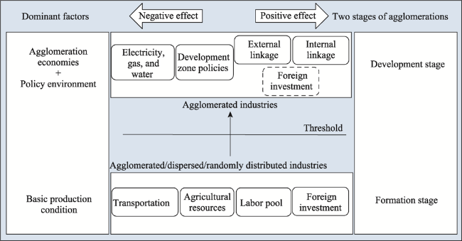
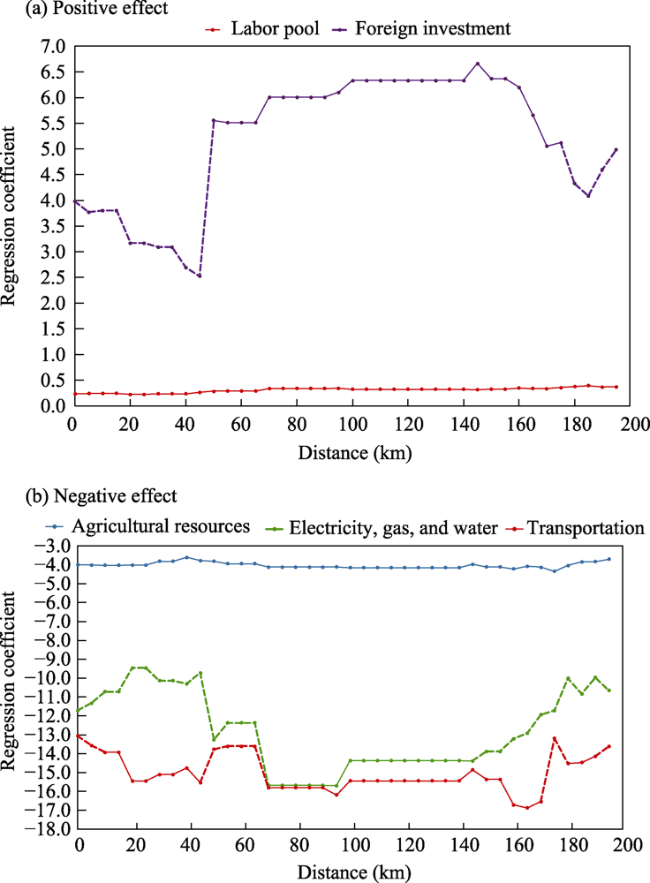
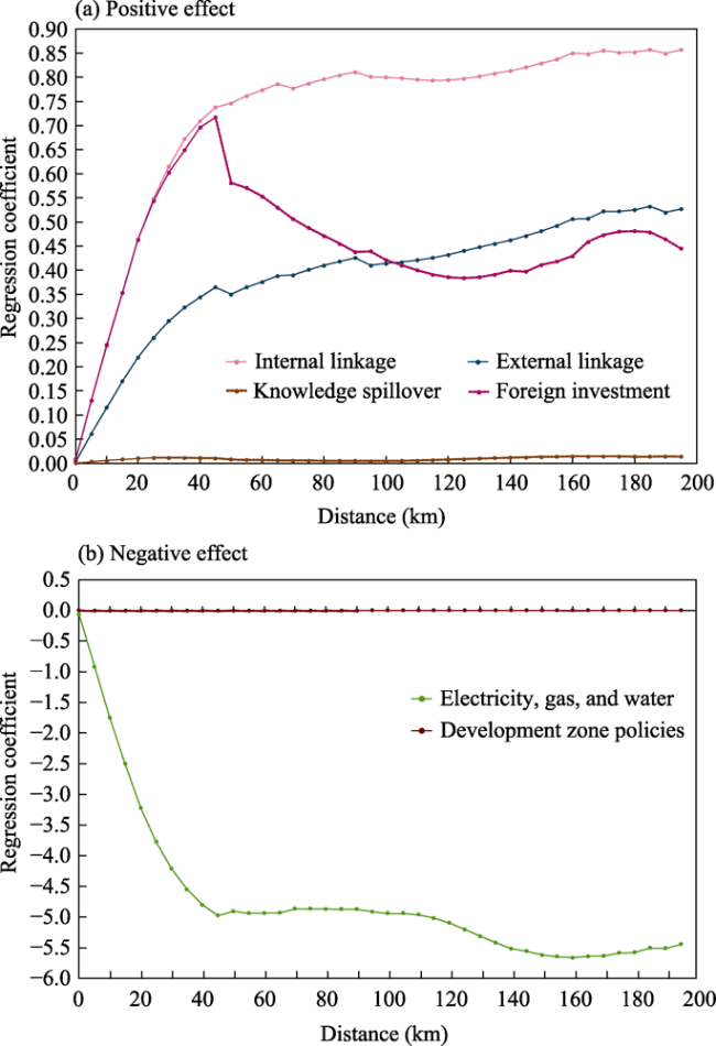
Industrial agglomeration is a highly prominent geographical feature of economic activities, and it is an important research topic in economic geography. However, mechanism-based explanations of industrial agglomeration often differ due to a failure to distinguish properly between the spatial distribution of industries and the stages of industrial agglomeration. Based on micro data from three national economic censuses, this study uses the Duranton-Overman (DO) index method to calculate the spatial distribution of manufacturing industries (three-digit classifications) in the Beijing-Tianjin-Hebei region (BTH region hereafter) from 2004 to 2013 as well as the hurdle model to explain quantitatively the influencing factors and differences in the two stages of agglomeration formation and agglomeration development. The research results show the following: (1) In 2004, 2008, and 2013, there were 124, 127, and 129 agglomerations of three-digit industry types in the BTH region, respectively. Technology-intensive and labor-intensive manufacturing industries had high agglomeration intensity, but overall agglomeration intensity declined during the study period, from 0.332 to 0.261. (2) There are two stages of manufacturing agglomeration, with different dominant factors. During the agglomeration formation stage, the main locational considerations of enterprises are basic conditions. Agricultural resources and transportation have negative effects on agglomeration formation, while labor pool and foreign investment have positive effects. In the agglomeration development stage, enterprises focus more on factors such as agglomeration economies and policies. Internal and external industry linkages both have a positive effect, with the former having a stronger effect, while development zone policies and electricity, gas, and water resources have a negative effect. (3) Influencing factors on industrial agglomeration have a scale effect, and they all show a weakening trend as distance increases, but different factors respond differently to distance.

Cite this article

HUANG Yujin , SHENG Kerong , SUN Wei . Influencing factors of manufacturing agglomeration in the Beijing-Tianjin-Hebei region based on enterprise big data[J]. Journal of Geographical Sciences, 2022 , 32(10) : 2105 -2128 . DOI: 10.1007/s11442-022-2039-9

1 Introduction

Industrial agglomeration is one of the most prominent geographical features of economic activities. It refers to a cluster of enterprises who engage in a type of division of labor to produce a certain commodity. The theoretical explanation of industrial agglomerations can be traced back to Marshall’s research on industrial districts in the late 19th century. He believed that external economies and economies of scale are the driving forces for industrial agglomeration. Subsequently, Weber’s theory of the location of industries, Schumpeter’s theory of innovation, and Hoover’s theory of the specific scale of specialized agglomeration all introduced reasonable and influential explanations of the phenomenon. Since the 1980s, interpretations of agglomeration mechanisms in geography and economics have diverged. Geographers have studied neo-industrial districts such as the “third Italy” and Silicon Valley in the United States and suggested that industrial agglomeration originates from the flexible specialization and vertical separation of production systems, summarizing agglomeration in terms of transaction costs and learning and innovation capabilities (Scott, 1988; Malmberg, 1997). Based on spatial economic models and centripetal and centrifugal force analysis, economists believe that industrial agglomeration is the result of historical and accidental factors, that they are the cumulative effect of industrial links, and that agglomeration mechanisms are increasing returns to scale, transportation costs, and path dependence (Krugman, 1997; Miao, 2003). In recent years, mechanism-based explanations of industrial agglomeration have added perspectives, such as globalization, institutional transformation, local protectionism, and proximity (Bai, 2004; He, 2008; Liu and Zhu, 2020). For example, Liang’s research showed that geographical concentrations of FDI have led the rapid agglomeration of capital-intensive and technology-intensive industries in China (Liang, 2003). Bai et al. (2004) found that local protectionism is more prevalent and the concentration of industrial regions is lower among industries with higher tax rates and greater nationalization. He et al. (2008) suggested that economic transformation could explain China’s industrial location and that marketization and globalization may stimulate industrial agglomeration, while decentralization may lead to protectionism and industrial dispersion.
Looking at the existing literature, it is evident that there are still differences in mechanism-based explanations of industrial agglomeration. This is due to different measurement methods as well as a lack of understanding about the status and stages of agglomerations. Regarding the former, Lu and Tao (2007) used the Ellison-Glaeser index to determine that the tobacco processing industry at the county level had the lowest agglomeration among all industries, with a value that was only one-thirtieth of the maximum value. He et al. (2007), meanwhile, calculated the tobacco industry’s Gini coefficient as being the highest of all industries. Therefore, a credible and widely accepted measurement method needs to be established. Regarding the latter, the spatial forms of industries (agglomeration, dispersion, and random distribution) are not fully considered with mechanism-based explanations. However, in reality, industries with a dispersed or random distribution and industries that are agglomerated are not consistent in mechanism-based explanations. Existing studies have shown that some industries are not prone to agglomeration. For example, Duranton and Overman (2005) constructed the DO index model based on geographic distance, and their study showed that only 52% of manufacturing industries in the UK are agglomerated at the 95% confidence level, while 24% are dispersed and 24% are randomly distributed. The proportion of manufacturing agglomeration in other manufacturing powerhouses around the world is mostly between 50% and 70%.
Based on the above considerations, we believe that research on the influencing factors of manufacturing agglomeration should answer two questions: Which factors influence the formation of manufacturing agglomerations? Which factors influence the increase in the intensity of manufacturing agglomeration? These two questions refer to the two stages of manufacturing agglomeration. The first stage is the formation of an industry agglomeration, and the second stage is the development of the industry agglomeration based on the first stage. There may be differences in the influencing factors of these two stages. Most of the existing literature mixes results from the two stages, and they do not strictly distinguish between them. Highlighting this point helps to clarify the reasons for differences in the mechanism-based explanations of agglomeration, and understanding policy implications helps to increase industrial development and regional competitiveness.
In view of this, this study used the DO index and hurdle model to conduct empirical research on the BTH region. The BTH region was chosen because it is one of the core industrial agglomeration areas in China. The region is a leader in the automobile manufacturing, equipment manufacturing, electronic information, and biomedical industries. With the implementation of an integrated and coordinated development strategy for the BTH region, the manufacturing industry has shifted from agglomeration to decentralization and re-aggregation, gradually forming a differentiated and tiered division of labor (Zhang et al., 2016). Due to data limitations, this study looks at the manufacturing industry in the BTH region during the period 2004-2013 to identify quantitatively the spatial distribution and agglomeration intensity, and it uses the hurdle model to analyze the factors that influence manufacturing agglomeration and differences in the two stages of agglomeration.
The following are the three main marginal contributions of this study. First, using the data of 414,000 manufacturing enterprises and the DO index method to identify quantitatively the scope and intensity of manufacturing agglomeration in the BTH region, it avoids the Modifiable Area Unit Problem (MAUP) caused by administrative divisions. Second, we propose that agglomeration can be divided into two stages, and we use the hurdle model to analyze quantitatively their influencing factors and differences in the different stages. Third, we identify the spatial scale effect of influencing factors on industrial agglomeration, which basically satisfies the Distance Decay Law, but with differences between the two stages.

2 Research methods and data sources

2.1 Industrial agglomeration measurement method

This study uses the DO index to measure the degree of agglomeration of various industries. The DO index measures industrial distribution form by comparing the distribution density of pairwise distances between actual enterprises in the industry and random enterprises. This method is different from traditional statistical approaches based on administrative units, with the model built instead on the continuous space of geographic distance. It is often used in cutting-edge research in industrial geography (Qiao et al., 2007; Cui et al., 2020; Liu and Wang, 2021; Zhao et al., 2021). This method consists of the following three main steps:
The first step is to construct a kernel density estimation function and calculate the spatial distribution curve of actual enterprises. If there are n companies in industry A, and the Euclidean distance between company i and company j is dij, the Gaussian kernel function f is used to calculate the density, and bandwidth h is set with reference to Silverman (1986). The Gaussian kernel function formula is as follows:
${{\hat{K}}_{A}}\left( d \right)=\frac{1}{n\left( n-1 \right)h}\underset{i=1}{\overset{n-1}{\mathop \sum }}\,\underset{j=i+1}{\overset{n}{\mathop \sum }}\,f\left( \frac{d-{{d}_{ij}}}{h} \right)$
The second step is to simulate a random distribution of enterprises using a random sampling technique. The location of enterprises is not completely random in space due to the influences of natural conditions and land use, so this study needs to control location selection caused by the impact of manufacturing. All actual enterprise locations are formed into a set, with the same number of enterprise points randomly selected for each simulation, and a simulated enterprise spatial distribution curve is calculated according to the first step. The process is repeated 1000 times.
The third step is to construct a global confidence interval and calculate the agglomeration index. A global confidence interval is a joint estimate of local extreme values over multiple distances. Specifically, the values of the 5% and 95% quantiles of the 1000-iteration simulation results at any distance are used as the upper and lower limits of the local confidence interval. The global confidence interval is obtained based on the interpolation of local extreme values at multiple distances. The confidence level is controlled at 95%. Since the sum of kernel density values over all distances is 1, if industry A is agglomerated at short distances, it appears to be scattered at long distances. Therefore, only the short-distance spatial distribution of the industry needs to be considered. The definition of short distance significantly affects the identification of spatial distribution characteristics. In this paper, 194 km, which is one-quarter of the diameter of the study area, was used as the maximum boundary. This is similar to the distances of 200 km and 180 km used in other studies (Duranton and Overman, 2005; Meng et al., 2019).
Assuming that the upper and lower limits of the global confidence interval are ${{\tilde{K}}_{A}}\left( d \right)$ and ${{\underset{\scriptscriptstyle\thicksim}{K}}_{A}}\left( d \right)$, respectively, if industry A exists ${{\hat{K}}_{A}}\left( d \right)>{{\tilde{K}}_{A}}\left( d \right)$at $d\in \left[ 0,194 \right]$, it is considered that industry A exhibits agglomeration characteristics at the 95% confidence level; if industry A does not exist at ${{\hat{K}}_{A}}\left( d \right)>{{\tilde{K}}_{A}}\left( d \right)$ at $d\in \left[ 0,194 \right]$, but ${{\hat{K}}_{A}}\left( d \right)<{{\underset{\scriptscriptstyle\thicksim}{K}}_{A}}\left( d \right)$ exists, it is considered that industry A exhibits dispersion characteristics. In other circumstances, industry A is considered to be randomly distributed, that is, neither agglomeration nor dispersion. Figure 1 shows the spatial distribution curves of four typical industries. Both the plastic products industry and the sporting goods manufacturing industry are globally agglomerated. The former has an agglomeration range of 0–165 km, and the latter has an agglomeration range of 0–194 km. The grain milling industry is globally dispersed, and the non-ferrous metal casting industry is randomly distributed.
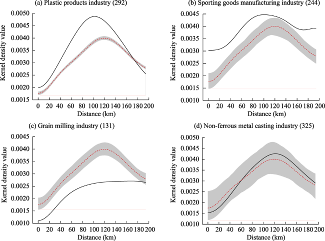
Figure 1 Spatial distribution curves of four typical industries

Note: The solid line represents the actual spatial distribution curve of the industry, the gray strip represents the 95% global confidence interval under random conditions, and the dotted line represents the average value of the confidence interval.

The equations for calculating the global agglomeration index (${{\Gamma }_{A}}\left( d \right)$) and the dispersion index (${{\Psi }_{A}}\left( d \right)$) are as follows:
${{\Gamma }_{A}}\left( d \right)\equiv \text{max}\left( {{{\hat{K}}}_{A}}\left( d \right)-{{{\tilde{K}}}_{A}}\left( d \right),0 \right)$
${{\Psi }_{A}}\left( d \right)\equiv \left\{ \begin{matrix} \text{max}\left( {{{\underset{\scriptscriptstyle\thicksim}{K}}}_{A}}\left( d \right)-{{{\hat{K}}}_{A}}\left( d \right),0 \right)\text{ if }\underset{d=0}{\overset{d=194}{\mathop \sum }}\,{{\Gamma }_{A}}\left( d \right)=0; \\ 0\ \ \ \ \ \ \ \ \ \ \ \ \ \ \ \text{ else} \\ \end{matrix} \right.$
This study uses the dbmss package for R to calculate the DO index (Marcon et al., 2015). The related commands divide the global distance into 512 parts and return kernel density values for each part of the distance. To simplify the calculation, this paper conducted research on the results of 512 dispersed distances.

2.2 Hurdle model

To improve the practical significance of the DO index model, this study learned from Alfaro and Chen (2014) to build an index for measuring industry A’s agglomeration intensity within any distance (S), which is used as the explained variable. The formula is as follows:
$D{{O}_{A}}\left( S \right)=\underset{d=0}{\overset{d=S}{\mathop \sum }}\,{{\Gamma }_{A}}\left( d \right)=\underset{d=0}{\overset{d=S}{\mathop \sum }}\,\left[ {{{\hat{K}}}_{A}}\left( d \right)-{{{\tilde{K}}}_{A}}\left( d \right) \right]$
About 20% of industrial agglomeration intensity is 0, which is typical for merged data. The Tobit model is often used to merge data, but it has strict requirements on the normality and homoscedasticity of the disturbance term. According to the conditional moment test and the construction of the LM statistic, it was found that the data has heteroscedasticity and non-normality issues, so a hurdle model, also known as a two-part model, was constructed (Cragg, 1971; Chen, 2010). As a generalization of the Tobit model, the hurdle model can avoid the above problems. The model’s formula is expressed as follows:
$f\left( y|x \right)=\left\{ \begin{matrix} P\left( d=0|x \right)\ \ \ \ \ \ \ \ \ \ \ \ \ \ \ \ \ \ \ \text{ if}\ y=0 \\ P\left( d=1|x \right)f\left( y|d=1,x \right)\text{ if}\ y>0 \\\end{matrix} \right.$
where d is the dummy variable, agglomerated industries (y>0) are denoted as d=1, dispersed or randomly distributed industries (y=0) are denoted as d=0, and P is probability.
The first stage in the hurdle model answers whether the independent variable is conducive to the formation of agglomeration based on the whole sample. All non-zero values of the explained variable are set to 1, and the Probit binary selection model is set:
$Probit\left( {{y}_{i}}=1|{{x}_{ni}} \right)=\lambda +{{\nu }_{n}}{{x}_{ni}}+{{\gamma }_{i}}$
The second stage, which is based on agglomeration industry samples (d=1), answers how the independent variable affects the degree of industry agglomeration. The explained variables are continuous variables and satisfy the assumptions of the linear model, and the ordinary least squares (OLS) method is used to estimate and set the linear model:
${{y}_{i}}=\alpha +{{\beta }_{n}}{{x}_{ni}}+{{\varepsilon }_{i}}$
where yi is the explained variable, λ and α are the constant terms, vn and βn (n=1, 2…) are the parameters to be estimated, xni are the independent and control variables, γi and εi are the error terms.

2.3 Data sources and processing

The data in this paper comes from three national economic censuses, which show almost complete enterprise and attribute information in China in a specific year. It is one of the most detailed and authoritative sources of survey data at the enterprise level, and it is widely used in industrial research. There are 414,000 pieces of information on manufacturing enterprises in the BTH region in the economic censuses. This study also uses forward geocoding for visualization based on enterprise address information, which is mainly based on the geocoding and location retrieval services provided by the Baidu Maps Open Platform (http://lbsyun.baidu.com/). In addition, about 0.62% of enterprises have zero or absent employees. We considered these enterprises to lack production and manufacturing capabilities temporarily, so they were removed from the data. Figure 2 shows the kernel density distribution of manufacturing enterprises in the BTH region in 2004, 2008, and 2013.
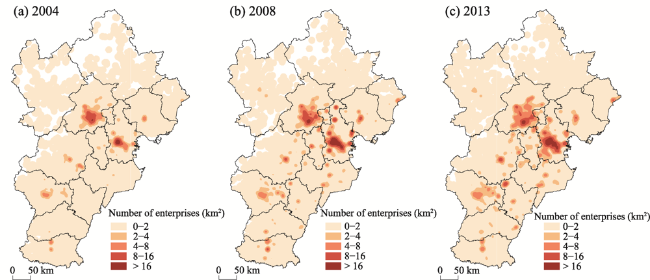
Figure 2 Kernel density distribution of manufacturing enterprises in the Beijing-Tianjin-Hebei region in 2004, 2008, and 2013
The research unit used in this study was based on the mid-level classification of manufacturing industries under China’s national industry classification system, which is distinguished by three-digit codes. The time span of this study was 2004-2013, which covers two industry classification standards. Given the need to match data, classifications of manufacturing industries in 2004 and 2008 use the National Industrial Classification of Economic Activities (GB/T 4574-2002) and those from 2013 use the National Industrial Classification of Economic Activities (GB/T 4574-2011). In addition, industries with too few enterprises (less than 10) (tobacco leaf processing, cigarette manufacturing, other tobacco product processing, and nuclear fuel processing) were considered unrepresentative, so they were removed. As a result, the sample contains 162 manufacturing industry types in 2004 and 2008, and 168 in 2013.

3 Research results

3.1 General features of manufacturing agglomeration

In accordance with the DO index model, the number and proportion of three-digit manufacturing industries with different spatial morphology characteristics were judged at the 95% confidence level. From 2004 to 2013, the number of industries with agglomeration characteristics increased from 124 to 129, and the proportion of all industries increased first and then decreased but with little fluctuation and hovered around 77% (Table 1).
Table 1 The number and agglomeration intensity of agglomerated, dispersed, and randomly distributed industries in the Beijing-Tianjin-Hebei region in 2004, 2008, and 2013
Year Agglomerated industries Dispersed industries Randomly distributed industries Total number of industries Average agglomeration intensity
Number Proportion Number Proportion Number Proportion
2004 124 76.5% 22 13.6% 16 9.9% 162 0.332
2008 127 78.4% 27 16.7% 8 4.9% 162 0.307
2013 129 76.8% 29 17.3% 10 6.0% 168 0.261
Table 1 shows that the spatial distribution of the manufacturing industry is selective, with most industries tending to agglomerate, and a few industries tending to be dispersed. From 2004 to 2013, the proportion of industries in manufacturing agglomerations in the BTH region was approximately 77%, which was much higher than that of the United Kingdom (52%) (Duranton and Overman, 2008), Canada (52%) (Behrens and Bougna, 2015), and Japan (50%) (Nakajima et al., 2012), but similar to Germany (71%) (Koh and Riedel, 2014), in the same period. This proportion was also higher than in the research results of Shao (44%) (2018), Chen et al. (65%) (2018), and Meng et al. (70%) (2019), or the research results of Wei et al. (16%) (2020) on the Yangtze River Delta urban agglomeration. It was similar, however, to the results of Brakman et al. (77%) (2017). Regarding the different agglomeration proportions, assuming the accuracy of the model’s method, the main reasons for the high manufacturing agglomeration in the BTH region are that the manufacturing industry in this region has a national comparative advantage, allowing it to attract a continuous stream of enterprises and resources to the region. Additionally, compared with the multi-core structure of the Yangtze River Delta urban agglomeration, the two core cities of Beijing and Tianjin in this region have a higher status, and the spatial structure of the urban agglomeration is relatively simple, so deciding where to locate manufacturing industries is more straightforward.
According to the equation ${{\Gamma }_{A}}=\underset{d=0}{\overset{d=194}{\mathop \sum }}\,{{\Gamma }_{A}}\left( d \right)$, the total agglomeration intensity of industry A can be obtained by accumulating the global agglomeration indices over all distances and averaging the strengths of all industries with agglomeration characteristics in each year. From 2004 to 2013, average overall agglomeration intensity continued to decrease, from 0.332 to 0.261, a decrease of about 21.4%. Different industries had different agglomeration intensities. In 2004, industries such as aerospace manufacturing, electronic computer manufacturing, bicycle manufacturing, bookbinding and other printing service activities, and other electronic equipment manufacturing industries had high agglomeration intensity. In 2013, manufacturing of wire rope and its products, bicycle manufacturing, motorcycle manufacturing, cultural and office machinery manufacturing, and metal furniture manufacturing had high agglomeration intensity. It can be seen that the highly agglomerated industries changed little between 2004 and 2013. They were mostly technology-intensive (transportation equipment, electronic equipment, and instrumentation) and labor-intensive (leather or fur and furniture) manufacturing industries (Table 2). This observation is consistent with the results of previous studies (He et al., 2008).
Table 2 Top 10 manufacturing industries in the Beijing-Tianjin-Hebei region in terms of agglomeration intensity
Industry classification 2004 Industry classification 2008 Industry classification 2013
Aerospace vehicle manufacturing 1.22 Leather tanning 1.09 Manufacturing of wire rope and its products 1.09
Electronic computer manufacturing 1.12 Bicycle manufacturing 1.07 Bicycle manufacturing 1.06
Bicycle manufacturing 1.10 Other unspecified manufacturing 0.94 Motorcycle manufacturing 0.90
Bookbinding and other printing service activities 1.07 Aerospace vehicle manufacturing 0.92 Cultural and office machinery manufacturing 0.78
Other electronic equipment manufacturing 1.01 Ship and floating device manufacturing 0.90 Metal furniture manufacturing 0.74
Ship and floating device manufacturing 1.01 Bookbinding and other printing service activities 0.84 Electronic component manufacturing 0.71
General equipment manufacturing 0.92 Electronic computer manufacturing 0.80 Leather goods manufacturing 0.69
Manufacturing of special instruments 0.91 Electronic component manufacturing 0.75 Aerospace vehicle and equipment manufacturing 0.66
Leather tanning 0.90 Medical instrument and equipment manufacturing 0.75 Fur tanning and product processing 0.66
Biological and biochemical products manufacturing 0.83 Metal furniture
manufacturing
0.65 Leather tanning 0.65

Note: The theoretical value range of overall agglomeration intensity in the 0-194 km range is 0-1, but to simplify the calculation in this study, the results of 512 dispersed distances were added, resulting in the expansion of the results to 2.63 times the original, which does not affect the intensity comparison.

We counted the number of agglomerated industries at different distances and added the indices of all agglomerated industries on each d according to the equation $\Gamma \left( d \right)=\underset{A=1}{\overset{A=m}{\mathop \sum }}\,{{\Gamma }_{A}}\left( d \right)$ to compare the relationship between the number/index of manufacturing agglomeration industries and the distance (Figure 3). The number of agglomerated industries and the agglomeration index decrease rapidly as distance increases in the range of 0–60 km, and they decrease gently at a distance of 60–194 km, though both have a “hump” at 110 km, especially in 2004 and 2008. The distance of 0–60 km is the most frequent and efficient distance for enterprise communication and industry associations, such as knowledge and technology learning, intermediate product transportation, labor and talent sharing, and other activities. At larger distances, transportation costs are the main limiting factor on enterprise links (Shao et al., 2018). In addition, placing these distances on real geographical spaces, changes in the number of agglomerated industries and the agglomeration index with distance correspond to the evolution process of industrial agglomeration from a single city to between multiple cities. The core area of urban industrial development is 0–60 km, where the agglomeration of factors of production generates substantial external benefits, and 110 km is almost the distance between two cities. The hump is caused by industrial agglomeration between two cities being greater than that of an urban fringe area within a city. This indirectly explains the industrial spatial links between cities.
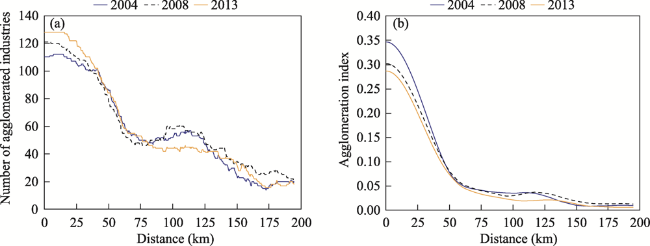
Figure 3 Number of agglomerated industries (a) and agglomeration index of industries (b) in the Beijing-Tianjin-Hebei region at different distances

3.2 Variable selection

Based on the existing literature, this study selected the four explanatory variables of resource endowment, agglomeration economies, government behavior, and globalization (Table 3). Resource endowment and agglomeration economies are common criteria for discussing industrial location, while government behavior and globalization reflect the reality of manufacturing development in China.
Table 3 Descriptions of core explanatory variables
Influencing factor Variable Quantitative indicator Name Data source
Resource
endowment
(RES)
Agriculture Intermediate inputs in agriculture, forestry, animal husbandry and fishery as a proportion of total industry inputs RES_AGR Regional input- output tables
Mining Intermediate inputs in coal, petroleum, metal, and non-metal as a proportion of total industry inputs RES_MIN
Electricity, gas, water Intermediate inputs in electricity, gas, and water supply as a proportion of total industry inputs RES_ENE
Agglomeration economies
(AGG)
Labor pool Number of employees in the industry AGG_EMP Economic census data
Internal links of industries Intermediate inputs in industries as a proportion of total inputs AGG_INI Regional
input-output tables
External links of industries Intermediate inputs of other manufacturing products as a proportion of total inputs AGG_INT
Knowledge spillover Number of industry patents AGG_TEC PatSnap patent platform
Government
behavior
(GOV)
Local
protectionism
State-owned enterprises in the industry as a proportion of all enterprises GOV_NAT Economic census data
Development zone policies Number of times the industry has become the target of a development zone GOV_LEV Catalogue of China Development Zones
Globalization (GLO) Foreign trade Industry exports value as a proportion of total sales value GLO_EXP Industrial enterprise database
Foreign
investment
Foreign-invested enterprises in the industry as a proportion of all enterprises GLO_FOR Economic census data

Note: To reduce the two-way causal relationship between independent variables and dependent variables, the variables derived from the micro-data of industrial enterprises are all lagged by one period.

According to the theories of comparative advantage and resource endowment, resources are a basic factor in determining the selection of location for enterprises, and differences in industries’ dependence on particular resources directly affect their spatial distribution. With the improvement of communication technology and transportation, the influence of natural resources is gradually diminishing, and the influence of inputs such as labor and capital are increasing (Kim, 1999). This study selected the variables of agriculture, minerals, and electricity, gas, and water, and used the input-output tables of three provinces and cities (for 2002, 2007, and 2012) to summarize and calculate the inputs of various natural resources as a proportion of total industry inputs.
The theory of agglomeration economies is often used to explain the micro-scale mechanisms of industrial location selection, and it holds that industrial agglomeration creates external benefits. Agglomeration reduces the cost of movements of labor (professional talent), intermediate goods, and knowledge and technology, which scholars refer to as labor pool sharing, industrial linkages, and knowledge spillovers. The labor pool variable was quantified by calculating the number of employees in various industries using economic census data (for 2004, 2008, and 2013). Industrial linkages include both internal and external linkages. For these, we used the input-output tables of the municipalities and province in the study area to calculate internal and external intermediate product inputs as proportions of total inputs (He et al., 2007). Knowledge spillovers are difficult to measure directly, so the number of patents granted is often used as a proxy (Fischer, 2009; Zhao and Bai, 2009). This article used the PatSnap patent platform (https://www.zhihuiya.com) to obtain numbers of patents granted to Beijing, Tianjin, and Hebei by the China National Intellectual Property Administration in 2004, 2008, and 2013.
As globalization has developed, the focus of economic activities since the 1980s has gradually shifted from Europe to the United States and then to Asia (Dicken, 2003). China has actively participated and gradually established institutional advantages, becoming the world’s largest recipient of foreign investment in 2003. Thanks to its abundant and cheap labor resources, globalization has driven the development of the manufacturing industry in China’s coastal areas, creating a manufacturing layout oriented toward resource inputs and agglomeration economies (He et al., 2008). This study selected foreign trade and foreign investment as variables to reflect globalization, which were quantified as industry exports as the proportion of total sales and the number of foreign-invested enterprises as a proportion of total enterprises, respectively (Liang, 2003; Xian and Wen, 2006).
Government behavior is an important force in regulating industrial development led by the market economy. Disorderly competition between China’s multi-level administrative systems and long-term use of GDP to assess performance has made the impact of government behavior on the spatial distribution of industries very complex (Zhou, 2007). On the one hand, local governments have increased agglomeration economies by establishing development zones and attracting enterprises with preferential policies (Lu et al., 2015; Li and Wu, 2018). On the other hand, competition has led local governments to protect state-owned enterprises and enterprises with high profits and tax rates, which has affected the agglomeration of industries (Bai et al., 2004). The development zone policy variable is quantified as the number of times an industry has become the leading industry of a park. The data source is the Catalogue of China Development Zones (2006 and 2018). The leading industries of development zones at or above the provincial level in the BTH region were counted according to their date of approval and were approximately matched using two-digit industry classifications.
The control variables in this study include spatial structure and transportation. The spatial structure variable represents the deviation caused by the difference in proportions of industries between the province and municipalities, and it is quantified as the proportion of industries in Beijing and the proportion of industries in Tianjin. The transportation variable is quantified as intermediate inputs as a proportion of total inputs.
The descriptive statistics of the variables are given in Table 4.
Table 4 Descriptive statistics of variables
Variable type Variable name Observations Average Standard deviation Minimum Maximum
Dependent variable DO (50) 492 0.170 0.222 0 1.201
DO (100) 492 0.204 0.248 0 1.203
DO (150) 492 0.224 0.262 0 1.224
DO (194) 492 0.231 0.264 0 1.224
Independent variable RES_AGR 492 0.053 0.094 0 0.311
RES_MIN 492 0.039 0.078 0 0.601
RES_ENE 492 0.030 0.0178 0 0.077
AGG_EMP 492 36953 56086 167 520480
AGG_INI 492 0.249 0.114 0 0.528
AGG_INT 492 0.254 0.147 0 0.543
AGG_TEC 492 167.4 537.8 0 5,600
GOV_NAT 492 0.015 0.026 0 0.333
GOV_LEV 492 28.68 40.29 0 138
GLO_EXP 492 0.165 0.180 0 0.898
GLO_FOR 492 0.062 0.052 0 0.339
SPA_BJ 492 0.231 0.165 0 0.870
SPA_TJ 492 0.256 0.137 0.022 0.775
RES_TRA 492 0.036 0.014 0 0.115

Note: The dependent variable DO(S) represent the industrial agglomeration intensity within the range of S calculated according to Formula 4.

3.3 Model regression results

Prior to the regression analysis, we performed a multicollinearity test on the explanatory variables. The correlation coefficients of independent variables in the model were all less than or equal to 0.6, and the variance inflation factor (VIF) was less than 10, so the issue of multicollinearity could be ignored. To reduce the effect of heteroscedasticity, the model used robust standard errors.

3.3.1 Influencing factors of manufacturing agglomeration

The first stage of the hurdle model answers the question of whether each influencing factor is conducive to the formation of agglomerations in the manufacturing industry. After 2011, due to changes in the statistical coverage of enterprises above a designated size and missing data for some variables (such as foreign trade (GLO_EXP)), there could be inconsistencies in the data from 2013 compared to 2004 and 2008. To ensure the robustness of the model, Table 5 lists the mixed cross-sectional regression results for the two periods of 2004-2008 and 2004-2013, respectively. The model considered the year fixed effect. The first stage used the maximum likelihood estimation method, and each model passed the chi-square test.
Table 5 Probit regression results of the first stage in the hurdle model
Model 2004‒2008 2004‒2013
(1) (2) (3) (4) (5) (6) (7) (8)
S 50 km 100 km 150 km 194 km 50 km 100 km 150 km 194 km
RES_AGR -3.813** -4.153** -4.106** -3.703** -3.042** -3.158** -3.119** -2.837*
(1.695) (1.734) (1.709) (1.694) (1.467) (1.488) (1.489) (1.509)
RES_MIN 1.325 1.262 1.201 0.915 0.249 0.162 0.153 0.202
(2.039) (2.099) (2.067) (1.995) (1.412) (1.432) (1.424) (1.413)
RES_ENE -13.264 -14.357* -13.884 -10.649 6.624 7.071 7.579 7.808
(8.470) (8.597) (8.643) (8.524) (5.391) (5.520) (5.511) (5.437)
AGG_EMP 0.287*** 0.321*** 0.328*** 0.373*** 0.240*** 0.252*** 0.258*** 0.311***
(0.086) (0.083) (0.084) (0.085) (0.058) (0.057) (0.057) (0.058)
AGG_INI 1.086 1.716 1.720 1.459 -0.637 -0.345 -0.428 -0.570
(1.706) (1.701) (1.690) (1.698) (1.278) (1.293) (1.298) (1.318)
AGG_INT 0.206 0.516 0.395 0.570 0.929 1.133 1.119 1.268
(1.609) (1.632) (1.608) (1.611) (1.377) (1.396) (1.399) (1.433)
AGG_TEC -0.014 -0.006 -0.028 -0.044 -0.061 -0.060 -0.069* -0.067
(0.077) (0.084) (0.084) (0.094) (0.041) (0.042) (0.042) (0.043)
GOV_NAT 0.651 0.756 0.224 0.883 -1.233 -1.382 -1.634 -0.937
(3.807) (4.088) (4.056) (3.903) (2.271) (2.284) (2.299) (2.266)
GOV_LEV -0.007 -0.010 -0.006 -0.002 -0.001 -0.002 -0.001 -0.001
Model 2004‒2008 2004‒2013
(1) (2) (3) (4) (5) (6) (7) (8)
(0.006) (0.006) (0.006) (0.007) (0.003) (0.003) (0.003) (0.003)
GLO_EXP 0.611 0.551 0.608 0.456
(0.585) (0.627) (0.621) (0.594)
GLO_ FOR 5.552** 6.333** 6.367** 4.989* 4.690** 4.830** 4.891** 3.434*
(2.780) (3.052) (3.089) (2.979) (2.003) (2.132) (2.150) (2.034)
SPA_BJ 2.568*** 2.583*** 2.592*** 2.204*** 2.501*** 2.491*** 2.515*** 2.357***
(0.672) (0.712) (0.713) (0.706) (0.517) (0.533) (0.534) (0.539)
SPA_TJ 1.751** 1.945** 1.658** 1.118 2.580*** 2.769*** 2.623*** 2.316***
(0.694) (0.756) (0.735) (0.718) (0.562) (0.583) (0.579) (0.583)
RES_TRA -13.759 -15.439* -15.359* -13.606 -12.833** -13.414** -13.757** -12.867**
(8.473) (8.735) (8.670) (8.390) (6.412) (6.547) (6.547) (6.558)
Constant -2.321** -2.652** -2.656** -2.771** -2.218** -2.353*** -2.342*** -2.525***
(1.118) (1.100) (1.092) (1.092) (0.894) (0.896) (0.897) (0.910)
Time fixed effect Yes Yes Yes Yes Yes Yes Yes Yes
Observations 324 324 324 324 492 492 492 492
Pseudo R2 0.224 0.247 0.241 0.219 0.223 0.237 0.236 0.229

Note: The numbers in brackets are robust standard error, *, **, and *** mean significant at the level of 10%, 5%, and 1% respectively, the same below.

Regarding the natural resources factor, agricultural resources inputs (RES_AGR) have a significant negative impact on the formation of manufacturing agglomeration, which gradually weakens as distance increases. Mineral resources (RES_MIN) and electricity, gas, and water (RES_ENE) have no significant impact on manufacturing agglomeration. This may be because natural resources are basic conditions for the development of manufacturing and their spatial distribution is relatively dispersed due to their regionality and scarcity. As a result, enterprises stay close to natural resources to reduce transportation costs and such industries are characterized by dispersion. Although transportation technology has facilitated long-distance transportation, easing the restrictions natural resources place on the distribution of industries, it is still an important factor when considering the layout of some industries, especially food-related industries (Table 6). Agricultural products rot and deteriorate, and they have higher transportation costs compared to mineral products and electricity, gas, and water, so they are more closely connected to local markets. As a result, industries with high inputs of agricultural resources are often dispersed.
Table 6 Agglomeration intensity of the top 5 two-digit industries in the agricultural resources input in 2013
Industry Proportion of agricultural resources input Agglomeration intensity within each distance
50 km 100 km 150 km 194 km
Agricultural and sideline food
processing industry
0.301 0.018 0.021 0.021 0.022
Food manufacturing 0.301 0.022 0.023 0.023 0.024
Beverage manufacturing 0.301 0.000 0.000 0.000 0.000
Textile industry 0.245 0.144 0.156 0.169 0.193
Textile clothing, shoes,
hats manufacturing
0.126 0.161 0.250 0.258 0.258
Average of all industries 0.057 0.152 0.180 0.195 0.200

Note: Only two-digit industries are involved in Input-Output Table. In this paper, the proportion of agricultural resource input is calculated by approximate matching method, and the agglomeration intensity is the average value of the three-digit industry.

In terms of the factor of agglomeration economies, labor pool (AGG_EMP) has a significant positive impact on the formation of manufacturing agglomerations, and that impact increases as distance increases. Internal industry linkages (AGG_INI), external industrial linkages (AGG_INT), and knowledge and technology spillovers (AGG_TEC) are not significant. The larger the enterprise, the stronger the demand for labor, and the greater the need to be close to densely populated areas. In addition, abundant labor resources in these areas also attract many enterprises, which can lead to industry agglomerations.
Looking at the globalization factor, foreign investment (GLO_FOR) has a significant positive impact on the formation of manufacturing agglomerations, which first strengthens and then weakens as distance increases. The pursuit of profits is the fundamental objective of capital flows. The motives of foreign investment in China can be summarized as production input and market, production service, favorable policies, and reduced investment risk (Wei et al., 2001). Therefore, industries with high added value and a strong agglomeration effect, such as the electronic communication equipment and chemical raw materials and products manufacturing industries, are favored by foreign investors (Liang, 2003). Foreign investment promotes industrial agglomeration and upgrading of the industrial structure by spreading advantages and removal, but the law of distance attenuation applies to these spillover effects (Liu et al., 2009). Overall, foreign investment makes crucial contributions to the growth, as well as the efficiency, speed, and quality of growth, of China’s manufacturing industry in the early stage (Li, 2003).
Of the control variables, the proportion of industry employees in Beijing (SPA_BJ) and the proportion in Tianjin (SPA_TJ) both have significant positive effects on the formation of manufacturing agglomerations. Beijing and Tianjin are important agglomeration locations of China’s manufacturing industries, with a wide variety of industries, strong supporting capabilities, and obvious development advantages. Their degree of industrial agglomeration is much higher than that of Hebei Province. As a result, the higher the proportion of industries in the two municipalities, the greater the likelihood of agglomerations forming. Transportation (RES_TRA) has a significant negative impact on the formation of industrial agglomerations, as industries with higher transportation costs need to be close to markets or raw materials to reduce costs.

3.3.2 Factors influencing the increase in manufacturing agglomeration

The second stage of the hurdle model determines the influence of the independent variables on the agglomeration intensity of agglomerated industries (partial sample). All models passed the F test, and Table 7 reports the regression results of the influencing factors in the second stage of the hurdle model.
Table 7 OLS regression results of the second stage in the hurdle model
Model 2004-2008 2004-2013
(1) (2) (3) (4) (5) (6) (7) (8)
S 50 km 100 km 150 km 194 km 50 km 100 km 150 km 194 km
RES_AGR -0.001 -0.009 -0.025 -0.027 -0.086 -0.041 -0.055 -0.058
(0.196) (0.210) (0.223) (0.225) (0.217) (0.220) (0.228) (0.227)
RES_MIN 0.413 0.439 0.389 0.402 -0.120 -0.089 -0.133 -0.126
(0.263) (0.285) (0.299) (0.290) (0.184) (0.191) (0.197) (0.198)
RES_ENE -4.905*** -4.938*** -5.619*** -5.443*** -3.143*** -3.165*** -3.724*** -3.403***
(1.191) (1.290) (1.289) (1.307) (0.925) (0.962) (0.972) (0.998)
AGG_EMP -0.011 -0.001 0.002 0.005 -0.015 -0.005 -0.001 -0.001
(0.013) (0.014) (0.014) (0.013) (0.009) (0.010) (0.010) (0.010)
AGG_INI 0.746*** 0.800*** 0.829*** 0.857*** 0.365** 0.470*** 0.498*** 0.524***
(0.199) (0.209) (0.211) (0.207) (0.182) (0.180) (0.181) (0.179)
AGG_INT 0.350** 0.414** 0.481*** 0.527*** 0.155 0.288 0.338* 0.385**
(0.163) (0.177) (0.183) (0.184) (0.189) (0.187) (0.189) (0.188)
AGG_TEC 0.008 0.004 0.013 0.014 -0.002 -0.005 -0.000 -0.001
(0.009) (0.010) (0.010) (0.010) (0.007) (0.007) (0.007) (0.007)
GOV_NAT 0.248 0.070 0.074 0.090 0.140 -0.127 -0.102 -0.121
(0.504) (0.533) (0.453) (0.443) (0.477) (0.532) (0.496) (0.497)
GOV_LEV -0.001 -0.002* -0.002** -0.002** -0.001 -0.001** -0.002*** -0.002***
(0.001) (0.001) (0.001) (0.001) (0.001) (0.001) (0.001) (0.001)
GLO_EXP -0.043 -0.028 -0.027 -0.018
(0.086) (0.096) (0.096) (0.094)
GLO_ FOR 0.581 0.421 0.411 0.445 0.611** 0.443 0.443 0.499
(0.379) (0.416) (0.412) (0.410) (0.290) (0.309) (0.312) (0.312)
SPA_BJ 0.224* 0.311** 0.342** 0.325** 0.198* 0.274** 0.315*** 0.305***
(0.123) (0.136) (0.136) (0.135) (0.103) (0.109) (0.110) (0.110)
SPA_TJ 0.259 0.413** 0.462*** 0.441*** 0.223 0.349** 0.395*** 0.384***
(0.171) (0.178) (0.165) (0.162) (0.139) (0.146) (0.139) (0.137)
RES_TRA -1.484 -2.003 -1.807 -1.899 -0.196 -0.846 -0.554 -0.580
(1.608) (1.688) (1.682) (1.663) (1.204) (1.268) (1.284) (1.311)
Constant 0.061 -0.039 -0.080 -0.115 0.190 0.074 0.027 -0.001
(0.134) (0.142) (0.146) (0.143) (0.122) (0.127) (0.128) (0.125)
Time fixed effect Yes Yes Yes Yes Yes Yes Yes Yes
Observations 248 253 255 267 377 382 384 398
R2 0.345 0.307 0.346 0.348 0.240 0.231 0.264 0.262
In terms of the natural resources factor, the electricity, gas, and water (RES_ENE) variable has a significant negative impact on increasing industrial agglomeration, and the impact is enhanced within a range of 150 km. The impact weakens beyond this distance. Compared with agricultural and mineral resources, electricity, gas, and water are essential raw materials in production. When the government sells industrial land, it usually takes care of power and water supplies, so electricity, gas, and water resources are not primary factors that enterprises look for when seeking locations and they do not have a significant impact on forming agglomeration. Nevertheless, some agglomerated industries, such as the chemical industry, have high demand for electricity, gas, and water. Enterprises seek locations with cheap resources to save money, and the dispersed distribution of cheap resources leads to a decrease in the industrial agglomeration intensity (Zou and Duan, 2020).
In terms of the agglomeration economies factor, the internal industry linkages (AGG_INI) and external industry linkages (AGG_INT) have a significant positive impact on increasing agglomeration intensity, and the influence increases as distance increases. The closer internal industry linkages are, the more transportation costs can be saved by increasing agglomeration intensity, which is also conducive to building local brands and enhancing competitiveness. The closer external industry linkages are, the easier it is to promote inter-industry synergistic agglomeration (Chen and Chen, 2012) and indirectly increase agglomeration intensity within the industry. A possible reason why the positive effects of internal and external industry linkages change with distance could be the result of the combined effects of Marshallian externalities and Jacobian externalities (Wu and Li, 2011). The former plays a leading role at short distances and the latter at long distances, strengthening the positive effect of industrial linkages on agglomeration. The greater the distance, the more obvious the enhancement effect of Jacobian externalities. Moreover, the difference in the results of the internal and external industry linkages in the two stages of the model indicates that they only have a promotional effect on agglomerated industries and have no effect on whether an industrial agglomeration forms. This may be because industrial linkages work based on a certain level of agglomeration, and they are not a primary driving force. The impact of knowledge spillover (AGG_TEC) on agglomeration intensity is still insignificant. A possible reason is that although many patents are granted in the BTH region every year, only a few are used for local industrial development, as most are used in places like the Yangtze River Delta and Pearl River Delta, whereas much of the technology in the BTH region relies on comes from elsewhere (Duan et al., 2019). Local knowledge and technology advantages have not been fully exploited, making it difficult to attract more enterprises. The labor pool (AGG_EMP) is not significant in the second stage, indicating that labor is similar to the production of raw materials; it is an initial locational factor considered by enterprises and only plays a role in whether an industry forms an agglomeration.
In terms of the government behavior factor, the variable of local protectionism (GOV_NAT) is still insignificant in the second stage of the model, and it remains insignificant after the profit and tax variable is added to the model (not listed in the table). The long-standing unequal political status of the three administrative entities in the BTH region limits competition between local governments and significantly weakens local protectionism, limiting its influence on industrial agglomeration (Bo and Chen, 2015). Another explanation is that coastal areas are closer to foreign markets than inland areas, so local governments are less motivated to adopt protectionist measures (Huang and Li, 2006). The development zone policy (GOV_LEV) variable has a significant negative impact on the increase of agglomeration intensity. The reason is that there is excessive overlap between leading industries of several development zones in the BTH region, mainly the electronic information, equipment manufacturing, automobiles, and new materials industries, and excessive competition leads to dispersion of industries. Meng et al., (2019) provided a different explanation. They suggested that development zone policies adjusted the center-periphery layout of industry created by market forces, as tax incentives reduce the operating costs of enterprises and increase the number of enterprises in peripheral areas, which decreases industrial agglomeration.
In terms of the globalization factor, foreign investment (GLO_FOR) only has a positive impact on agglomeration intensity at a range of less than 50 km, and it is not significant at other distances. Foreign trade (GLO_EXP) also does not significantly increase agglomeration intensity. Like the first stage, the positive effect of foreign investment on industrial agglomeration declines with distance, though the rate of decline is faster. When an industry forms an agglomeration, domestic-funded enterprises grow by virtue of their local advantages, and the agglomeration gradually expands. The leading role of foreign-funded enterprises, meanwhile, continuously weakens so that they only play a role with enterprises at short distances (Wu and Li, 2011). The main reason for the significant difference between the effects of the foreign investment and foreign trade variables is that most of the trade in China’s coastal provinces is driven by foreign capital. There is a complementary relationship between the two, and foreign investment is the core factor affecting the distribution of export-oriented manufacturing industries (Huang and Li, 2006).
The effects of the three control variables on the improvement of industrial agglomeration are like those in the first stage, the only difference being that the negative impact of the transportation (RES_TRA) variable is not significant, indicating that it has no obvious restrictive effect on agglomeration. A further decrease in transportation costs may not promote the agglomeration of manufacturing industries, indicating that manufacturing in the BTH region may have crossed the left side of the inverted U-shaped curve described by new economic geography (Wen, 2004).

3.3.3 Comparative analysis of the two stage of manufacturing agglomeration

The regression results of the DO index and hurdle model verified that there are two stages of industrial agglomeration, and the dominant factors in the agglomeration formation stage and the agglomeration development stage are different (Figure 4).
Figure 4 Schematic diagram of two stages of manufacturing agglomeration
The initial formation of a manufacturing agglomeration is affected by agricultural resources, the labor pool, foreign investment, and transportation. Agricultural resources and transportation have a negative effect on the formation of manufacturing agglomerations, while the labor pool and foreign investment have a positive effect. When the spatial distribution of an industry crosses the agglomeration threshold, the agglomeration development stage is mainly affected by electricity, gas, and water resources, internal and external industry linkages, and development zone policies. The role of internal industry linkages is greater, and development zone policies and electricity, gas, and water resources play a negative role.
The two stages of industrial agglomeration reflect a change in enterprise decision-making regarding location. When there are no obvious agglomeration activities, the locational considerations of enterprises are the basic conditions needed to operate and survive. When an industrial agglomeration forms, the main locational considerations are agglomeration economies and the policy environment, as they seek to maximize profitability. This process can involve the entry of new firms and the exit of old firms. Of course, some industries, such as food manufacturing, have extremely high agglomeration thresholds that cannot be crossed, so they are more prone to a dispersed or random distribution.

3.3.4 The scale effect of influencing factors

Based on the regression results in different distance ranges (Tables 5 and 7), it can be preliminarily determined that the impact of each variable on industrial agglomeration has a scale effect. In the first stage, the influence of agricultural resources, foreign investment, and transportation on the formation of agglomerations first strengthens and then weakens as distance increases, so it is likely that there is an optimal range of agglomeration, while the positive effect of the labor pool constantly increases as distance increases. In the second stage, the effects of electricity, gas, and water and development zone policies on the formation of agglomerations also strengthens and then weakens as distance increases, while the positive effect of internal and external industry linkages continuously increases, but the positive effect of foreign investment rapidly weakens. The above indicates that the effects of variables do not completely conform to the law of distance decay, as some increase within a certain range while others continuously increase. He et al., (2007), and Fan and Li (2011) also suggested that the dominant factors that cause industrial agglomeration differ depending on whether one is looking at a small geographic area or a large geographic area.
Figure 5 The relationship between the regression coefficient of independent variables and the distance in the formation stage of agglomerations

Note: Figure a show the variables that can have a positive effect on the dependent variable, and Figure b shows the variables that have a negative effect. The dotted line in the figure indicates that the regression coefficient is not significant, and the solid line indicates that the regression coefficient is significant at 10% or 5%, the same as below.

Figure 6 The relationship between the regression coefficient of independent variables and the distance in the agglomeration development stage
To further verify the scale effect of influencing factors, this study calculated agglomeration intensity at intervals of 5 km from 0-194 km and established a model. Figures 5 and 6 show the relationship between the regression coefficient of independent variables and the distance in the two stages of the hurdle model (variables that were not significant in the range of 0-194 km are not shown).
We found that the change in the regression coefficient of each variable as distance changes is consistent with the above conclusions, which again shows that the effect of each influencing factor on industrial agglomeration has a scale effect. Following more detailed regression analysis, we found that the knowledge spillover variable only has a significant positive impact within 25 km. Although the effects of other variables have a stage in which they increase, they almost all tend to weaken as distance increases, such as internal industry linkages in Figure 6a. In addition, we can summarize the spatial scales at which different variables have a significant effect on industrial agglomeration. In the first stage, the coefficients of labor pool and agricultural resources are all significant in the range of 0-194 km, while the coefficients of foreign investment, electricity, gas and water, and transportation are only significant in the range of 50-150 km. In the second stage, the coefficients of internal and external industrial linkages and electricity, gas and water are significant in the range of 0-194 km, while the coefficient of the development zone policies variable is significant in the range of 90-194 km, and the coefficients of foreign investment and knowledge spillover are only significant at short distances, as they are very sensitive to spatial scale. Specifically, the positive effect of foreign investment in the agglomeration development stage rapidly strengthens in the range of 0-45 km, but the effect is significantly weakened and insignificant beyond 45 km. The positive effect of knowledge spillover on increasing industrial agglomeration is also evident in the range of 0-25 km, but it is not noticeable beyond 25 km. These empirical results show that the positive effects of variables on industrial agglomeration are strictly limited by distance.

4 Conclusions and discussion

4.1 Conclusions

Based on enterprise big data from three national economic censuses, this paper identified and measured the spatial distribution of manufacturing industries (to the three-digit classification) in the BTH region. We identified the two-stage characteristic of factors affecting industrial agglomeration and looked at differences in the roles of various factors at different spatial scales. Our research indicated the following:
(1) In the BTH region in 2004, 2008, and 2013, 124, 127, and 129 industries were clustered, 22, 27, and 29 industries were dispersed, and 16, 8, and 10 industries were randomly distributed, respectively. The agglomeration intensity of technology-intensive (transportation equipment, electronic equipment, instrumentation, etc.) and labor-intensive (leather and fur, furniture, etc.) manufacturing industries was relatively high, and the agglomeration range was mostly 0-60 km.
(2) Agglomeration can be divided into two stages: the agglomeration formation stage and the agglomeration development stage. In the agglomeration formation stage, agricultural resources and transportation have a negative effect on the formation of industrial agglomerations, while labor and foreign investment have a positive effect. Once an industry crosses the agglomeration threshold, i.e., in the agglomeration development stage, internal and external industry linkages (particularly internal industry linkages) have a positive effect, and development zone policies as well as electricity, gas, and water resources have a negative effect. In general, in the agglomeration formation stage, the main locational consideration of enterprises is basic conditions, whereas in the agglomeration development stage, they focus on agglomeration economies and the policy environment. Further research revealed that not all industries enter the second stage, and they will tend to be dispersed or randomly distributed if the cost of crossing the agglomeration threshold is too high.
(3) The effect of distance differs depending on the variable, but almost all show a weakening trend as distance increases. In the agglomeration formation stage, the influence of agricultural resources, foreign investment, and transportation all first increase and then decrease as distance increases, and the positive effect of the labor pool variable continuously increases but it slows with distance. In the agglomeration development stage, electricity, gas, and water and development zone policies also first increase and then decrease with distance, while the positive effects of knowledge spillover and foreign investment increase rapidly and then become insignificant, and the positive effects of both internal and external industry linkages continuously increase but slow with distance. Moreover, the various variables have significant effects on industrial agglomeration at specific spatial scales. In the first stage, the labor pool and agricultural resources variables have a significant effect within the range of 0-194 km, while the variables of foreign investment, electricity, gas and water, and transportation only play a role in the 50-150 km range. In the second stage, the variables of internal and external industry linkages as well as electricity, gas, and water have a significant effect at any distance; development zone policies only play a role in the range of 90-194 km; and foreign investment and knowledge spillover, which are particularly sensitive to spatial scale, are only significant in the 0-45 km and 0-25 km range, respectively.

4.2 Discussion

The two-stage nature of processes widely exists and is gradually attracting the attention of geographers (Gu and Shen, 2021). The hurdle model essentially assumes that there are two decision mechanisms for the restricted dependent variable, so a two-stage regression strategy is required. Regarding the influencing factors of industrial agglomeration, the existing literature often assumes that all industries tend to agglomerate. This is not the case, however. For example, most food-related industries tend to have a dispersed distribution. We believe that when discussing influencing factors of industrial agglomeration, we should first answer the reasons for the formation of an industrial agglomeration (as opposed to a random or dispersed distribution) and then analyze the mechanisms that cause greater agglomeration intensity. This study only focused on industrial agglomeration, but with the implementation of regional integration policies, the process of industrial dispersion and its influencing mechanisms are also worthy of attention. It is worth noting that although the two stages in the hurdle model can be assigned to the formation and development of industrial agglomerations, their connotations are not completely consistent. The former is more inclined to the logical sequence, and the latter is more inclined to the temporal dynamic process. How to unify the two and incorporate them into a hurdle model to analyze mechanisms of action will be our focus for future research.
This study also found that factors that influence industrial agglomeration have a scale effect. Although almost all of them weaken as distance increases, there are differences in their responses to distance. For example, in the second stage, the positive effects of internal and external industry linkages on agglomeration increase as distance increases, while the effects of electricity, gas, and water and development zone policies first strengthen and then weaken as distance increases. We also found that regardless of how a variable’s effect changes with distance, it tends toward a stable value, that is, a stable effect on industrial agglomeration. To an extent, this explains why there are consistent conclusions regarding the influencing factors of industrial agglomeration at different spatial scales in the literature. Nevertheless, factors that are highly sensitive to spatial scale need to be observed at specific spatial scales. For example, knowledge spillover only has a significant effect on industrial agglomeration within a range of 25 km, so incorrect conclusions could be drawn at larger spatial scales, such as prefecture-level cities. Of course, the lack of notable knowledge spillover effect in the BTH region could be due to the low local conversion rate of patents. This type of factor is especially significant in relation to industrial layout, so geography needs to pay special attention to such variables.
[1]
Alfaro L, Chen M X, 2014. The global agglomeration of multinational firms. Journal of International Economics, 94(2): 263-276.

DOI

[2]
Bai Chongen, Du Yingjuan, Tao Zhigang et al., 2004. Local protectionism and industrial concentration in China: Overall trend and important factors. Economic Research Journal, (4): 29-40. (in Chinese)

[3]
Behrens K, Bougna T, 2015. An anatomy of the geographical concentration of Canadian manufacturing industries. Regional Science and Urban Economics, 51: 47-69.

DOI

[4]
Bo Wenguang, Chen Fei, 2015. The coordinated development among Beijing, Tianjin and Hebei: Challenges and predicaments. Nankai Journal (Philosophy, Literature and Social Science Edition), (1): 110-118. (in Chinese)

[5]
Brakman S, Garretsen H, Zhao Z, 2017. Spatial concentration of manufacturing firms in China. Papers in Regional Science, 96: S179-S205.

DOI

[6]
Chen Guoliang, Chen Jianjun, 2012. Industrial relationship, spatial geography and secondary and tertiary industries agglomeration: Experience from 212 cities in China. Management World, (4): 82-100. (in Chinese)

[7]
Chen Ke, Zhang Xiaojia, Han Qing, 2018. The measure and characteristics of the geographical concentration of Chinese industries. Shanghai Journal of Economics, 30(7): 30-42. (in Chinese)

[8]
Chen Qiang, 2010. Advanced Econometrics and Stata Application. Beijing: Higher Education Press. (in Chinese)

[9]
Cragg J G, 1971. Some statistical models for limited dependent variables with application to the demand for durable goods. Econometrica, 39(5): 829-844.

DOI

[10]
Cui Zhe, Shen Lizhen, Liu Zishen, 2020. Spatial agglomeration characteristics of service industry in Xinjiekou CBD of Nanjing City and change: Based on micro enterprise data. Progress in Geography, 39(11):1832-1844. (in Chinese)

DOI

[11]
Dicken P, 2003. Global Shift: Reshaping the Global Economic Map in the 21st Century. London: Sage.

[12]
Duan Dezhong, Chen Ying, Du Debin, 2019. Regional integration process of China’s three major urban agglomerations from the perspective of technology transfer. Scientia Geographica Sinica, 39(10): 1581-1591. (in Chinese)

DOI

[13]
Duranton G, Overman H G, 2005. Testing for localization using micro-geographic data. The Review of Economic Studies, 72(4): 1077-1106.

DOI

[14]
Duranton G, Overman H G, 2008. Exploring the detailed location patterns of UK manufacturing industries using microgeographic data. Journal of Regional Science, 48(1): 213-243.

DOI

[15]
Fan Jianyong, Li Fangwen, 2011. Effect of spatial concentration of manufacturing in China: A review. South China Journal of Economics, (6): 53-66. (in Chinese)

[16]
Fischer M M, Scherngell T, Jansenberger E, 2009. Geographic localisation of knowledge spillovers: Evidence from high-tech patent citations in Europe. The Annals of Regional Science, 43(4): 839-858.

DOI

[17]
Gu H Y, Shen T Y, 2021. Modelling skilled and less-skilled internal migrations in China, 2010-2015: Application of an eigenvector spatial filtering hurdle gravity approach. Population Space and Place, 27(6): e2439. DOI: 10.1002/psp.2439.

DOI

[18]
He C, Wei Y D, Xie X, 2008. Globalization, institutional change, and industrial location: Economic transition and industrial concentration in China. Regional Studies, 42(7): 923-945.

DOI

[19]
He Canfei, Pan Fenghua, Sun Lei, 2007. Geographical concentration of manufacturing industries in China. Acta Geographica Sinica, 62(12): 1253-1264. (in Chinese)

[20]
Huang Jiuli, Li Kunwang, 2006. Foreign trade, local protectionism and industrial location in China. China Economic Quarterly, 5(2): 733-760. (in Chinese)

[21]
Kim S, 1999. Regions, resources, and economic geography: Sources of US regional comparative advantage, 1880-1987. Regional Science and Urban Economics, 29(1): 1-32.

[22]
Koh H-J, Riedel N, 2014. Assessing the localization pattern of German manufacturing and service industries: A distance-based approach. Regional Studies, 48(5): 823-843.

DOI

[23]
Krugman P R, 1997. Development, Geography, and Economic theory. Cambridge: MIT Press.

[24]
Li Ben,Wu Lihua, 2018. Development zone and firms’ growth: Research on heterogeneity and mechanism. China Industrial Economics, (4): 79-97. (in Chinese)

[25]
Li Haijian, 2003. Transnational corporations’ entrance and their impacts on Chinese manufacturing industries. China Industrial Economics, (5): 15-21. (in Chinese)

[26]
Liang Qi, 2003. Gini-coefficient of Chinese manufacturing industry: On the influence of FDI on manufacturing agglomeration. Statistical Research, 20(9): 21-25. (in Chinese)

[27]
Liu Guimei, Wang Maojun, 2021. Spatial agglomeration model of Japanese enterprises in Beijing based on enterprise point data. World Regional Studies, 30(5): 925-936. (in Chinese)

DOI

[28]
Liu Junyang, Zhu Shengjun, 2020. Proximity between markets and the geographical agglomeration of exporters in Guangdong province. Geographical Research, 39(9): 2044-2064. (in Chinese)

DOI

[29]
Liu Siyang, Lu Jiangyong, Tao Zhigang, 2009. Spillovers of FDI on indigenous manufacturing firms: A perspective of geographic distance. China Economic Quarterly, 8(1): 115-128. (in Chinese)

[30]
Lu Jiangyong, Tao Zhigang, 2007. Determinants of industrial agglomeration in china: Evidence from panel data. China Economic Quarterly, 6(3): 801-816. (in Chinese)

[31]
Lu Y, Wang J, Zhu L M, 2015. Do place-based policies work? Micro-level evidence from China’s economic zones program. SSRN Electronic Journal. doi: 10.2139/ssrn.2635851.

DOI

[32]
Malmberg A, 1997. Industrial geography: Location and learning. Progress in Human Geography, 21(4): 573-582.

DOI

[33]
Marcon E, Traissac S, Puech F et al., 2015. Tools to characterize point patterns: Dbmss for R. Journal of Statistical Software, 67(3): 1-15.

[34]
Meng Meixia, Cao Xiguang, Zhang Xueliang, 2019. Does the special economic zones policy affect industrial agglomeration in China: Based on the agglomeration perspective of the cross administrative boundary. China Industrial Economics, (11): 79-97. (in Chinese)

[35]
Miao Changhong, Cui Lihua, 2003. Industrial agglomeration: A viewpoint comparison between geography and economics. Human Geography, 18(3): 42-46. (in Chinese)

[36]
Nakajima K, Saito Y U, Uesugi I, 2012. Measuring economic localization: Evidence from Japanese firm-level data. Journal of the Japanese and International Economies, 26(2): 201-220.

DOI

[37]
Qiao Bin, Li Guoping, Yang Nini, 2007. The Evolution and new development of the industry agglomeration measurement. The Journal of Quantitative & Technical Economics, (4): 124-133,161. (in Chinese)

[38]
Scott A J, 1988. Flexible production systems and regional development. International journal of urban and regional research, 12(2): 171-186.

DOI

[39]
Shao Chaodui, Su Danni, Li Kunwang, 2018. Agglomeration across the border: Spatial characteristics and driving factors. Finance & Trade Economics, 39(4): 99-113. (in Chinese)

[40]
Silverman B W, 1986. Density Estimation for Statistics and Data Analysis. New York: Chapman and Hall.

[41]
Wei Haitao, Xiao Tiancong, Hu Baosheng et al., 2020. A distance-based measure of industrial agglomeration. Urban Development Studies, 27(10): 55-63. (in Chinese)

[42]
Wei Houkai, He Canfei, Wang Xin, 2001. An analysis of motives and location factors of foreign direct investment in China: An empirical study of foreign direct investment in Qinhuangdao city. Economic Research Journal, (2): 67-76, 94. (in Chinese)

[43]
Wen M, 2004. Relocation and agglomeration of Chinese industry. Journal of Development Economics, 73(1): 329-347.

DOI

[44]
Wu Sanmang, Li Shantong, 2011. Specialization, diversity and industrial growth. The Journal of Quantitative & Technical Economics, 28(8): 21-34. (in Chinese)

[45]
Xian Guoming, Wen Dongwei, 2006. FDI, regional specialization and industrial agglomeration. Management World, (12): 18-31. (in Chinese)

[46]
Zhang Jiefei, Xi Qiangmin, Sun Tieshan et al., 2016. Industrial division and transfer of manufacture in Beijing-Tianjin-Hebei region. Human Geography, 31(4): 95-101,160. (in Chinese)

[47]
Zhao Yong, Bai Yongxiu, 2009. Knowledge spillovers: A survey of the literature. Economic Research Journal, 44(1): 144-156. (in Chinese)

[48]
Zhao Ziyu, Wang Shijun, Chen Xiaofei, 2021. Beyond locality in restructuring the spatial organization of China’s automobile industry clusters under modular production: A case study of FAW-Volkswagen. Acta Geographica Sinica, 76(8): 1848-1864. (in Chinese)

DOI

[49]
Zhou Lian, 2007. Governing China’s local officials: An analysis of promotion tournament model. Economic Research Journal, 42 (7): 36-50. (in Chinese)

[50]
Zou Hui, Duan Xuejun, 2020. Layout evolution and its influence mechanism of chemical industry in China. Scientia Geographica Sinica, 40(10): 1646-1653. (in Chinese)

DOI

Outlines

/