Regular Articles

A spatio-temporal assessment and prediction of Ahmedabad’s urban growth between 1990-2030

  • Shobhit CHATURVEDI , 1, 2 ,
  • Kunjan SHUKLA 2 ,
  • Elangovan RAJASEKAR 1 ,
  • Naimish BHATT 2
Expand
  • 1.Department of Architecture and Planning, Indian Institute of Technology, Roorkee 247667, India
  • 2.Department of Civil Engineering, School of Technology, Pandit Deendayal Petroleum University, Gandhinagar 382007, India

Shobhit Chaturvedi (1991-), PhD Candidate, specialized in regional sustainable development and urban remote sensing. E-mail:

Received date: 2022-01-26

  Accepted date: 2022-05-15

  Online published: 2022-11-25

Supported by

Zero Peak Energy Demand for India (ZED-I)and Engineering and Physics Research Council EPSRC(EP/R008612/1)

Abstract

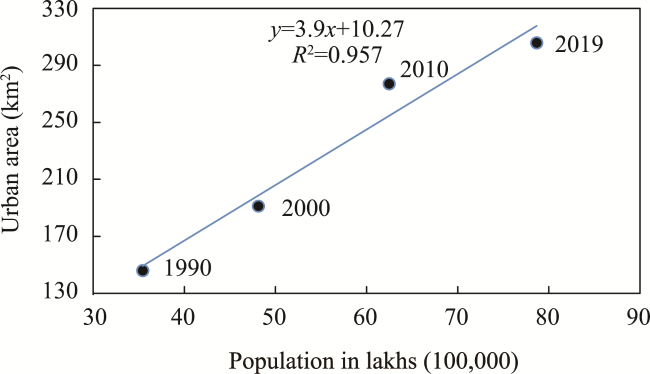
Analyzing long term urban growth trends can provide valuable insights into a city’s future growth. This study employs LANDSAT satellite images from 1990, 2000, 2010 and 2019 to perform a spatiotemporal assessment and predict Ahmedabad’s urban growth. Land Use Land Change (LULC) maps developed using the Maximum Likelihood classifier produce four principal classes: Built-up, Vegetation, Water body, and “Others”. In between 1990-2019, the total built-up area expanded by 130%, 132 km2 in 1990 to 305 km2 in 2019. Rapid population growth is the chief contributor towards urban growth as the city added 3.9 km2 of additional built-up area to accommodate every 100,000 new residents. Further, a Multi-Layer Perceptron - Markov Chain model (MLP-MC) predicts Ahmedabad’s urban expansion by 2030. Compared to 2019, the MLP-MC model predicts a 25% and 19% increase in Ahmedabad’s total urban area and population by 2030. Unaltered, these trends shall generate many socio-economic and environmental problems. Thus, future urban development policies must balance further development and environmental damage.

Cite this article

Shobhit CHATURVEDI , Kunjan SHUKLA , Elangovan RAJASEKAR , Naimish BHATT . A spatio-temporal assessment and prediction of Ahmedabad’s urban growth between 1990-2030[J]. Journal of Geographical Sciences, 2022 , 32(9) : 1791 -1812 . DOI: 10.1007/s11442-022-2023-4

1 Introduction

Land use refers to the utilization of Earth’s land resources for different human activities, whereas land cover is the bio-physical cover over Earth’s surface by built-up spaces, agricultural farmlands, green pastures, forests, water bodies etc. (Herold et al., 2006; Mishra and Rai, 2016). Together, land use land cover (LULC) change explains the modification of the Earth’s terrestrial surface by natural and anthropological means. Urbanization is the prime contributor to anthropogenic driven LULC changes, extending and densifying existing urban areas. Urbanization involves the mass migration of people towards urban areas searching for better job education and health care opportunities (Mansour et al., 2020). Urbanization expands existing city boundaries, transforming forests, croplands and wetlands into built-up areas containing residential, commercial and industrial buildings and supporting infrastructure like roads, bridges, parks, playgrounds etc. (Wakode et al., 2014).
Rapid population growth is regarded as the most significant contributor to urban expansion. (Hegazy and Kaloop, 2015; Nurwanda and Honjo, 2020). Since 1850, the total human population has increased six times globally, whereas the total urban population has grown 100 times (Ahmad, Goparaju and Qayum, 2017). By 2050, 66% of the global population is expected to live in cities that will present large-scale urban management challenges, especially in developing countries experiencing much faster urban growth than those faced anytime during the 20th century (Hassan et al., 2016; Shukla and Jain, 2019). Though urbanization provides several socio-economic benefits for the citizens, unplanned-uncoordinated, haphazard development can force city-dwellers to face several unintended negative consequences. Unplanned urban growth deteriorates urban dwellers’ quality of life by widening the gap between the demand and supply of essential services (Wakode et al., 2014). Under such situations, the urban population gets limited access to critical infrastructure facilities, including health, education, transportation and sanitation (Vermeulen et al., 2015; Saravanan et al., 2016; Islam and Dinar, 2021). Moreover, densely populated urban areas face a much higher risk of rapid transmission of infectious diseases like Covid-19. As seen in India, large numbers of infected people risk overhauling the available public health facilities hampering early detection, isolation, treatment and vaccination (Gupta et al., 2021). Rapid urbanization has also been linked to a widening socio-economic gap, proliferation of slums and rising crime rates (Hegazy and Kaloop, 2015; Kuddus et al., 2020).
Perhaps, the most damaging effect of unregulated-haphazard urbanization is visible in the urban environment. Urbanization replaces forests, agricultural and wetlands with built-up spaces, damaging flora-fauna biodiversity causing air, water, soil and noise pollution (Zhu et al., 2012; Power et al., 2018; Mansour et al., 2020). Further, unhealthy modifications to natural biogeochemical and hydrological cycles damage urban ecosystems (Ahmad et al., 2017). Many studies endeavoured to quantify the effects of rapid urbanization on natural resource quantity and quality, especially agricultural production, coastal contamination, air and water pollution and access to drinking water (Kaliraj et al., 2017; Power et al., 2018; Kookana et al., 2020). Rapidly declining agricultural land has also become a chief contributor to the global food shortage (Meshesha et al., 2016; Shi et al., 2016; Tarawally et al., 2019). Urbanization is also the prime contributor to Urban Heat Island (UHI). Due to urbanization, roads, pavements and building structures replace open lands, forest floors and farmlands with waterproof materials like pavements, asphalt, and concrete. Such changes decrease the ground absorptance, surface evaporation and heat-storage rates, thereby modifying the near-surface temperatures and wind flow patterns. UHI can increase the urban land surface temperatures (LSTs) by an average of 2-4℃ above neighboring rural areas (Rahman et al., 2017). UHI is also linked to health issues like heat strokes, asthma, and heart-related deaths, especially among children and elders (Ahmed et al., 2013; Borbora and Das, 2014; Rahman, Aldosary and Mortoja, 2017; Pal and Ziaul, 2017; Sultana and Satyanarayana, 2020).
Reliable LULC information is vital for sustainable urban planning to ensure sufficient resources for present and future generations (Han et al., 2015). The United Nations’ eleventh sustainable development goal also emphasizes periodic urban area monitoring to ensure environmentally responsible development (Tarawally et al., 2019). Assessing long-term LULC changes can assist urban planning efforts by identifying existing and potential social, infrastructure and environment-related challenges. Past changes to the regional landscape also provide a fair indication regarding the city’s future urban growth. However, physically monitoring LULC change is expensive, time-consuming, exhausting and prone to errors (Suribabu et al., 2012). Instead, multispectral and multi-temporal remote sensing (RS) satellite images provide a fast, precise and in-expensive solution to measure human activities’ influence on the Earth’s land resources (Mishra and Rai, 2016; Ahmad et al., 2017; Rahman et al., 2017). RS-Geographical Information System (GIS) tools reveal urban growth patterns by measuring the distance between urban areas away from the city centers (Hegazy and Kaloop, 2015). RS-GIS tools also help analyze large inaccessible areas to gauge their sensitivity/vulnerability to ongoing development trends (Wakode et al., 2014). Advanced RS-GIS predictive tools can also predict future urban expansion and help build sustainable land-use, transportation, infrastructure policies (Shafizadeh Moghadam and Helbich, 2013; Alqurashi and Kumar, 2014; Al shawabkeh et al., 2019).
Several Indian cities witnessed a drastic rise in population during the past two-three decades, leading to unprecedented levels of urban expansion (Shafizadeh Moghadam and Helbich, 2013; Mishra and Rai, 2016; Ahmad et al., 2017). As per United Nations world urbanization prospects, more than half of India’s population is expected to live in urban areas by 2050 (Shukla and Jain, 2019). Rapid population growth will stress already fragile urban infrastructure and the surrounding environment, especially after the Covid-19 pandemic. The developing nations should not be expected to replicate the growth trajectories exhibited by developed countries (Welsh, 2004). The success of any urban planning strategy for a region relies on a close understanding of its past and ongoing urban development. To this end, spatio-temporal LULC assessment can help analyze past and prevailing urban dynamics and provide future growth trends. Such studies can help regional and national governments with sustainable developmental planning. With almost one-third of India’s population residing in cities, it is crucial to acquire information regarding its growth patterns and environmental interactions (Wakode et al., 2014). This study performs a spatio-temporal assessment of a large Indian metropolitan city, i.e. Ahmedabad, to address the following research questions.
1. Which land-use classes are most affected by Ahmedabad’s urban growth during 1990-2019?
2. What is the relation between population rise and urban growth?
3. How much additional urban growth is expected for Ahmedabad by the end of the present decade, i.e. 2030?
The rest of the paper is structured as follows. A concise literature review is presented in section II, covering different approaches and methodologies for analyzing past and future LULC change dynamics. Section III contains a step-wise description of the methodology adopted for this study. Section IV explains the results of the spatiotemporal assessment and future LULC prediction. Finally, the closing Section V presents conclusions, recommendations, limitations and future scope.

2 Literature review

Research studies investigating the effects of LULC change on regional landscape, climate change and environmental damage have grown in number since the International Geosphere and Biosphere (IGB) program (Seitzinger et al., 2015; Silva et al., 2020). Most studies have focused on performing regional spatio-temporal assessment by comparing LULC maps from different periods. A few studies also focused on predicting future urban expansion employing advanced urban growth models. Most LULC change assessment and prediction studies are carried out using LANDSAT datasets. LANDSAT is the longest-running remote sensing program operated by the United States Geological Survey (USGS) and National Aeronautics and Space Administration (NASA) for acquiring Earth’s satellite imagery. Since the LANDSAT-1 mission launched in 1972, this program has provided free mid-resolution satellite images to perform spatio-temporal evaluations for several decades (Wakode et al., 2014). The most recent satellite LANDSAT 8, was launched on February 11 2013 (Wikipedia, 2021c).

2.1 LULC classification

LULC classification using suitable image classification techniques helps extract useful real-world information from multispectral satellite images. Several methods are available to classify mid (30 m × 30 m) and high resolution (15 m × 15 m) satellite imagery into a finite number of land use (LU) classes based on similar spectral reflectance profiles (MohanRajan et al., 2020). Broadly, LULC classification can be performed using unsupervised and supervised methods. Unsupervised LULC classification methods include K-Means clustering, ISODATA (Iterative Self-Organizing Data Analysis), Fuzzy C-Means clustering, Self-Organizing Maps and Neural Networks. Unsupervised classifiers such as ISODATA automatically classify satellite imagery into a user-defined number of groups based on similar spectral characteristics (Hegazy and Kaloop, 2015). Post classification, manual edits may be needed to remove a few miss-classified pixels or merge similar LU classes. In the past, researchers used the ISODATA algorithm for LULC classification of urban and coastal landscapes in India, Egypt and the middle east (Baby, 2015; Hegazy and Kaloop, 2015; Usman et al., 2015; Rahman, 2016; Ahmad et al., 2017).
Supervised LULC classification methods include the Maximum Likelihood Classifier (MLC), K-Nearest Neighbour, Support Vector Machines and Random Forest Classifiers (MohanRajan et al., 2020). These supervised methods can extend or extrapolate available LU information from known image sectors to classify unknown image sectors. In these methods, the user first develops a training set containing several training areas for each LU class. Next, the software generates class wise spectral signatures based on the provided training set. Finally, the software classifies the entire image by assigning each pixel to the LU class having maximum likelihood (Rahman, 2016). The supervised ML classifiers can be accessed using inbuilt tools present in QGIS, ArcGIS, and ERDAS Imagine software (MohanRajan et al., 2020). ML classifiers have been used for spatiotemporal assessment of hilly regions in Ramnagar and Almora, India, during 1990-2010 (Tripathi and Kumar, 2012; Rawat et al., 2013). ML classifiers have also been used to characterize LU changes in urban, forest and coastal landscapes across Indian cities like Tiruchirappalli, Hyderabad, Salem and Kanyakumari (Suribabu et al., 2012; Wakode et al., 2014; Kaliraj et al., 2017; Arulbalaji, 2019). In almost every study, the built-up area expanded at the expense of other LU classes such as forests, agriculture, water bodies, and wetlands. Unsupervised classifiers are helpful when no prior ground information is available. However, the process of identifying and recombining similar LU classes can be exhausting and generally produces lower classification accuracy. Notably, MLC is the most widely adopted LULC classifier for different landscapes as it delivers high accuracy by referring to LU signatures supplied by the user (Dewan and Yamaguchi, 2009; Belal and Moghanm, 2011; Tahir et al., 2013; Alqurashi and Kumar, 2014; Wakode et al., 2014; Usman et al., 2015; Meshesha et al., 2016; Shi et al., 2016; Kaliraj et al., 2017; Al shawabkeh et al., 2019; GeoKnowledge, 2020).

2.2 LULC prediction

In addition to the LULC classification, several researchers adopted advanced urban growth models to predict future urban growth (Mansour et al., 2020). These models can perform space-time simulations to determine long term LU class-wise transitional probabilities and generate future LULC maps. A few models solely rely on past LULC maps, whereas others also incorporate the influences of static (slope) and dynamic (urban density, road networks, proximity to main roads) urban growth drivers (Chang-Martínez et al., 2015; MohanRajan et al., 2020). The most common model, i.e. Cellular Automata- Markov Chain (CA-MC), is a spatio-temporal extension of the Markov Chains model that accommodates neighbourhood transition effects (Araya and Cabral, 2010; Nwaogu and Pechanec, 2017; Bhugeloo et al., 2019). This hybrid model solves the limitations of the CA model by integrating the effects of natural and human variables for making land use forecasts. For instance, Mansour et al. adopted a CA-MC model to simulate urban expansion during 2008-2038 in Nizwa city, Oman (Mansour et al., 2020). This model also considers the effects of elevation, aspects, terrain slopes, population density and proximity to roads and major urban centers. While implementing MC models, Multi Criteria Decision Making techniques and fuzzy logic may be needed to assign relative weights to different urban growth drivers. For instance, Moghadam and Helbich used an integrated MC-CA urban growth model to predict Mumbai’s urban expansion during 2020-2030 (Shafizadeh et al., 2013). The analytical hierarchy process apportioned the effects of different urban change drivers to develop transition probability maps.
The next popular class of urban growth models, i.e. MLP-MCA, relies on a neural network backpropagation algorithm to select suitable input parameters for predicting future urban growth. Using historical LULC maps and specific urban change drivers, the MLP-MCA method performs a non-parametric regression between several input parameters and one output, i.e. predicted pixel class membership (Losiri et al., 2016). For instance, Abd EL-kawy et al. used the Land Change Modeller module in Terrset software to implement an MLP-MC model to predict urban encroachment of agricultural lands in two different cities of Egypt between 2019 to 2100 (Abd EL-kawy et al., 2019). Similarly, L Silva et al. performed land change assessment and prediction for the Taperoá River basin of Brazil from 1990 to 2035 (Silva et al., 2020). Training for 1000 iterations, the backpropagation MLP algorithm produced future LULC maps with a high prediction accuracy of 89.69%. Ahmed et al. performed a comparative assessment of MLP-MC with stochastic Markov-Chain and CA-MC and models to predict Dhaka’s urban growth in 2019-2029 using LANDSAT images from 1989-2009. MLP-MC outperformed the other two models when validated against an actual 2009 LULC image (Ahmed and Ahmed, 2012).
Few specialized urban growth models can also develop future LULC maps based on different theories of urban development (Han et al., 2015). These models can incorporate the effects of possible policy changes by the government about urban development and environmental exploitation (Mohamed and Worku, 2020). Urban growth models have also been linked to the UHI phenomenon for predicting LSTs (Pal and Ziaul, 2017; Gohain et al., 2021). For instance, B. Ahmed et al. employed the MLP-CA model to simulate Dhaka’s urban growth during 2019-2029 (Ahmed et al., 2013). Empirical relationships between urban growth drivers and urban LSTs indicated that up to 56% and 87% of the total urban area may encounter temperatures above 30 °C in 2019 and 2029, respectively. Several other urban growth models such as GEOMOD, LCM, CLUES, Dynamica, EGO, and GISCAME have also been employed to predict future land use. Extensive discussions on the suitability of different LULC prediction methods can be found by referring to the works of Chang-Martínez et al. (2015) Nwaogu and Pechanec (2017), and MohanRajan et al. (2020). Various instances from the literature confirm the suitability of MLC and MLP-MCA algorithms for LULC classification and prediction. Therefore, this study selects these models for Ahmedabad’s spatio-temporal assessment and prediction.

3 Methodology

3.1 Study area

The city of Ahmedabad (23.022°N, 72.571°E) is located in the western Indian state of Gujarat, along the banks of the Sabarmati river. Placed in north-central Gujarat, the state capital is roughly 53 meters (174 ft) above the mean sea level. Built on sandy and dry soils, the entire city has a flat landscape except for some small hills located in the northwestern area. The city experiences a hot, semiarid type climate (Köppen climate classification: BSh), having three primary seasons, i.e. summer, winter and monsoons. Apart from monsoons, the weather is warm and dry, especially during summers (April-June) when the daily maximum temperature frequently rises above 40℃. The city receives an average yearly precipitation of 932 mm (Wikipedia, 2021b). Ahmedabad is a major economic center, home to many textile, pharmaceuticals and information technology companies generating a gross domestic product of $68 billion (in 2017). It hosts many public sector enterprises with central research and training institutions, universities, and professional colleges. Modern shopping and office centers, educational institutes, housing facilities and old heritage buildings, along with ample transportation facilities, including metro, buses, shuttles and an international airport, all contribute to the city’s socio-economic development.
The city’s population has grown steadily since the 1950s, achieving a 2.54% annual growth rate to reach 8,059,441 in 2020, making it the fifth most densely inhabited Indian city and 46th worldwide (Wikipedia, 2021d). Further, Ahmedabad also has a high slum population. The last publically available estimates from 2013 suggest 262,551 people living in slums around the city (Mahadevia et al., 2014). Rapid unplanned urban growth shall burden the city’s existing civic, health and transportation infrastructure and also damage its natural ecology. The prevailing land-intensive urban growth strategy shall intensify city-wide pollution (air, water, noise) levels and embolden UHI-induced climate changes. Investigating past urban growth trends can provide valuable insights into prevailing and future urban growth. Thus, this study gauges Ahmedabad’s 1990, 2000, 2010 and 2019 LU maps to predict the city’s urban growth in 2030 and 2040. Noteworthy, the city’s present-day total urban extent is equal to 464 km2. However, the official city boundaries get redrawn every few years as per new development plans. So, this study considers a total area of 945 km2 around the city’s centre to fully estimate the effects of ongoing and probable future expansions.
As shown in Figure 1, a step-wise framework is adopted for performing a spatio-temporal assessment and future prediction of Ahmedabad’s urban growth. The entire methodology is divided into three main steps.
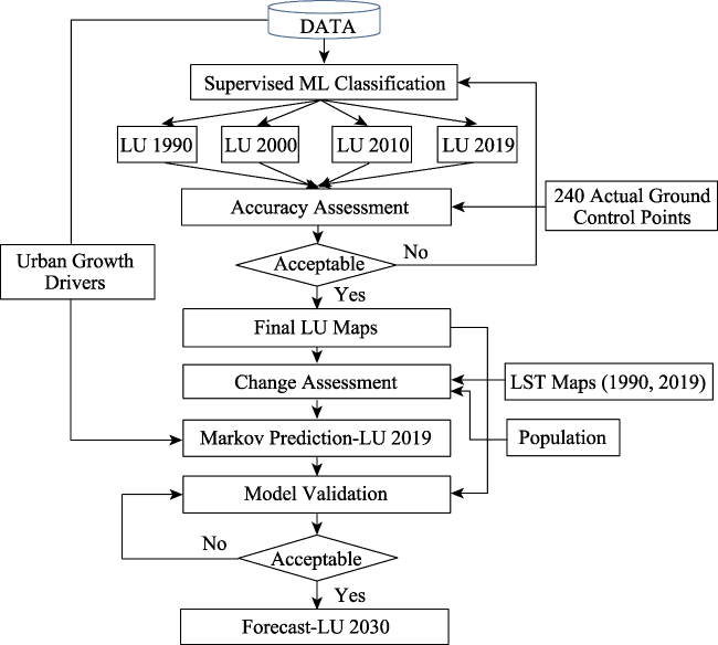
Figure 1 Overall workflow for this study
Several existing mid-resolution (30 m × 30 m) LANDSAT satellite datasets are downloaded from the United States Geological Survey (USGS) Earth Explorer repository during the first stage. The LANDSAT program consists of a series of earth-observing satellite missions managed by the USGS and NASA. Since 1972, this program has provided free mid-resolution satellite images for spatio-temporal evaluations (Wakode et al., 2014; Tarawally et al., 2019). LANDSAT 8 Operational Land Imager and Thermal Infrared Sensor images are acquired for 2019 and 2011, whereas the earlier 2000 and 1991 images are obtained from the LANDSAT 4-5 mission Thermic Mapper sensor. All four images belong to the (10-20) May period. Further, Ahmedabad’s digital elevation model (DEM) and road network map are procured from NASA and OpenStreetMap websites, respectively (Haklay and Weber, 2008). As shown in Table 1, Ahmedabad’s population data from 1990 to 2019 is taken from the world population review database (World Population Review, 2021).
Table 1 Different data sources used in this study
Dataset Time stamp Sensor/Source Resolution
LANDSAT 1990 LANDSAT 4-5 Thermic Mapper (TM) (30 × 30) m
LANDSAT 2000 LANDSAT 4-5 Thermic Mapper (TM) (30 × 30) m
LANDSAT 2010 LANDSAT 8 Operational Land Imager and Thermal Infrared Sensor (30 × 30) m
LANDSAT 2019 LANDSAT 8 Operational Land Imager and Thermal Infrared Sensor (30 × 30) m
Population data 1990, 2000, 2010, 2019 World Population Review 2021 Yearly
Digital Elevation Model ASTER ASTER (NASA) (30 × 30) m
Road network 2019 OpenStreetMap Vector
All four satellite images are geo-referenced to the Universal Transverse Mercator (UTM) projection system with World Geodetic System (WGS) 1984 as the datum. The particular area of interest is clipped by Erdas Imagine 2015 software using a common shapefile. Next, specific multispectral bands are combined to develop four satellite images of false-colour composite (FCC) images. The convolution and thematic tools are used for image sharpening and smoothening (Hegazy and Kaloop, 2015). Further, the Maximum Likelihood Algorithm is used for supervised LULC classification of the four FCC satellite images.

3.2 LULC classification: Maximum likelihood supervised classification

LULC maps for 1990, 2000, 2010 and 2019 are generated post supervised classification of the four FCC satellite images. Erdas Imagine 2015 software performs image classification by implementing the Maximum Likelihood (ML) algorithm. ML algorithm extrapolates user-supplied LU information from known image sectors to classify unknown image sectors (Wakode et al., 2014; Kaliraj et al., 2017). Initially, the user develops a training set containing several training areas for each LU category. Then the software generates class wise (LU) spectral signatures based on the supplied information. Next, the software classifies the entire image by assigning each pixel to the LU class having maximum likelihood (Rahman, 2016).
As shown in Table 2, ML algorithm classified the four FCC images into four LU broad categories: Vegetation, Water body, Built-up area and Bare land. The Vegetation class comprises all land use consistent with trees, forests, gardens, farmland, agricultural land, while all rivers, lakes, canals, and wetlands fall under Water body. The third LU class, i.e. Built-up area, contains all different buildings and physical infrastructure like roads, bridges, airports, etc. The final LU class, i.e. “Others”, contains open areas, bare plots, uncropped-farmlands landfill areas, and other remaining land uses.
Table 2 The four unique LU classes used for classifying the LANDSAT images
Land cover type Description
Water body Water bodies including rivers, lakes, canals and wetlands
Vegetation Green cover including trees, forests, gardens, cropped agricultural farmlands
Built-up area Physical infrastructure inclusive of roads, bridges, residential, commercial, industrial and institutional buildings
Others Open areas, including uncropped agricultural lands, bare plots, landfill areas and all other remaining land cover types
The confusion matrix approach can evaluate the quality and usability of classified LULC images by calculating the kappa statistics (Congalton and Green, 2019). Kappa statistic is calculated by dividing the total number of correctly classified pixels by the total number of reference pixels. Two hundred fourty actual ground points (60 points per LU class) are generated randomly to compare the actual and predicted LU class labels. Kappa statistic values closer to 0 and 1 indicate near perfect and random assignments. A minimum kappa value of 0.75 is necessary for accepting the ML algorithm’s classification results. The next step performs LULC change assessment by comparing the extents of the four LUs classes during the four periods. Further, LU class transitions are explained using transition probabilities during 2000-2010 and 2010-2019 shown in the LU transition matrix.

3.3 Multi-layer perceptron-Markov chain model

MLP-MCA model is suitable for quantifying long term spatio-temporal LULC change and predicting future urban growth (Mishra and Rai, 2016; Mansour et al., 2020). MLP-MCA is implemented using the Terrset 2018 software package. There are three main stages in performing the MLP-MC analysis. (1) Change Analysis; (2) Transition Area Analysis; (3) Change Prediction Analysis (Nurwanda and Honjo, 2020). During the change analysis stage, transformations between different LU classes are assessed between 2000 and 2010. Markov Chain analysis is used in the following transition analysis stage to obtain the LU change transition area matrix. The transition area matrix can be represented using equation 1.
$A=\text{ }\!\!~\!\!\text{ }\left[ \begin{matrix} {{\text{A}}_{11}} & \cdots & {{\text{A}}_{1\text{n}}} \\ \vdots & 0 & \vdots \\ {{\text{A}}_{\text{n}1}} & \cdots & {{\text{A}}_{\text{nn}}} \\ \end{matrix} \right]$
where Aij > 0, $\underset{j=1}{\overset{n}{\mathop \sum }}\,{{A}_{ij}}$= 1, $i=1,\ldots,n.$ Aij represents the transition probability between states i and j. After developing the transition matrix, the MLP-MC model is applied to predict future LU maps. For the change prediction assessment, only major LU transitions are considered, such as bare land to built-up spaces, Vegetation to built-up spaces, bare lands to Vegetation and Vegetation to bare lands.
Further, the MLP-MCA model also considers several urban change drivers impacting growth (Dadhich and Hanaoka 2010). DEM, slope maps and road and urban distance maps are tested as potential urban-change drivers. Cramer V statistic calculates the association level between land-use change and driving factors. A significance value closer to 0 implies that the variable has a weak association with the LU change (Mishra and Rai, 2016). All urban change drivers with Cramer V values greater than 0.15 are useful (Eastman, 2009). Next, a neural network is developed during the change prediction stage to train an MLP model (Ahmed and Ahmed, 2012). During the MLP training, the input signals from the input layer are passed to the next layer nodes in a feed-forward manner (Atkinson and Tatnall, 1997; Araya and Cabral, 2010; Hegazy and Kaloop, 2015). The input received by a single node is represented in equation 2.
$ne{{t}_{i}}=\mathop{\sum }^{}{{w}_{ik}}{{o}_{k}}$
where wik is the wight between node k and node l and ok is the output from node k. Further, output from node l, i.e., ol is illustrated in equation 3 (Atkinson and Tatnall, 1997).
${{o}_{k}}=f\left( ne{{t}_{i}} \right)$
Generally, a non-linear sigmoid function f(neti) is applied to the weighted sum of inputs before passing the inputs to the next layer. This step is termed Forward Propagation. Once all nodes send a forward signal, the output is compared to the actual response (a set of training data, e.g. known LU classes). This difference, termed network error, is transmitted back into the network. After that, the weight of each node is adjusted as in equation 4.
$\Delta {{w}_{ij}}\left( n+1 \right)=\alpha \Delta {{w}_{ij}}\left( n \right)+\eta \left( {{\delta }_{j}}{{O}_{i}} \right)$
where η=learning rate parameter; δj=error rate of change index; α=momentum parameter. This forward and backward propagation process is repeated iteratively until the network errors get minimalized to an acceptable scale. The end goal of these iterations is to find proper connection weights for all nodes between the input, hidden and output layers. Post MLP training, transition probability maps are developed for all the locations. Terrset uses a fuzzy membership function for every pixel. A higher class value represents a higher membership to the particular LU class. Final MLP network outputs and final LU maps for 2019 and 2030 are simulated using the Markov-Chain analysis. Before 2030 LU maps is developed, MLP-MC projected 2019 LU map is compared to the actual 2019 LU map to ensure sufficient prediction accuracy. LU class-wise accuracy is calculated by equating the actual and predicted area of each LU category.

4 Results

4.1 Spatiotemporal mapping of LULC changes

Figures 2, 3 and Table 4 describe the region’s urban growth during the past three decades, i.e. 1990-2019. All the four (1990, 2000, 2010, 2019) LULC maps are classified into four broad LU classes: Vegetation, Water body, Built-up, and Others. The actual LU class of the 240 randomly generated ground points is verified using Google Earth Explorer to calculate Kappa statistics. As shown in Table 3, all four years overall Kappa values are higher than 0.80, and Built-up LU class kappa values are always greater than 0.85, implying a close match between classified and actual ground features. All four ML generated LULC maps are acceptable, as their overall Kappa values are higher than the minimum threshold of 0.80 (Congalton and Green, 2019).
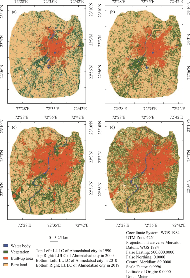
Figure 2 Ahmedabad LULC maps between 1990-2019
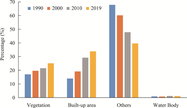
Figure 3 Temporal change of land use classes during the four periods
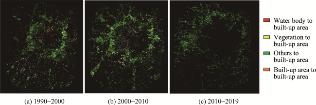
Figure 4 Transformation of different LULC classes to the Built-up spaces
Table 3 The calculated Kappa statistic values for the four years
LU class Class-Wise Kappa coefficient
1990 2000 2010 2019
Water body 0.83 0.75 0.87 0.91
Vegetation 0.82 0.78 0.90 0.74
Built-up area 0.85 0.86 0.86 0.95
Others 0.80 0.82 0.82 0.86
Overall Kappa 0.83 0.80 0.86 0.87
Table 4 Absolute quantities for each LU class during 1990-2019
LU class Area (km2)
Year
1990 2000 2010 2019
Water body 9.47 8.23 12.03 11.24
Vegetation 161.03 185.55 203.84 226.60
Built-up area 132.45 181.55 276.46 305.24
Others 641.49 569.10 452.10 357.47
The total area under study is 945 km2. During 1991, the “Others” LU class covered the largest 641.49 km2 followed by the built-up class covering 132.45 km2, vegetation class cover of 161.03 km2 and 9.37 km2 of water bodies. Several interesting patterns emerge from Table 4 and Figure 2. In the past 30 years, Ahmedabad’s total built-up area has grown extensively both in extent and density. As shown in Figure 3, the Built-up class grew from 181.45 km2 in 2000 to 276.46 in 2010 and 305.24 km2 in 2019. During 1990-2019, the region’s total Built-up area more than doubled, showing 130% growth, with an average decadal gain of 33%. The urban growth rate was fastest during 2000-2010, i.e. 52%, followed by 37% and 10% during 1990-2000 and 2010-2009.
The second-largest change is seen in the “Others” LU class, containing open areas such as bare plots, uncultivated agricultural lands and landfills. The total “Others” area reduced to half its size during 1990-2019, with a 17% average decadal decrease rate. The highest percentage decrease of 21% is seen during 2010-2019, trailed by 20% and 11% during 1990-2000 and 2000-2019. The “Others” LU class reduction also indicates a net decrease in cultivable lands as this LU class contain large amounts of un-cropped farmlands, as verified by Google Earth Explorer. Next, a rising trend is seen for the Vegetation LU class comprising cropped agricultural farmlands, parks and forests. Vegetation class enlarged by 40.8% from 161.03 km2 in 1990 to 226.60 km2 during 2019. With the highest growth rate of 15.3% during 1990-2000, this class continues to grow at a decadal growth rate of 12%, due to several afforestation programs run by the local government and municipal corporation. The final LU class, i.e. Water body comprising river, lakes, canals and wetlands, cover a tiny fraction of the city’s area ~1%. In comparison to other classes, this LU does not show much fluctuation. However, after the construction and interlinking of the Narmada river with the Sabarmati, the Water body class total area increased 46.2% during 2000-2010. As a result, the Sabarmati river no longer runs dry anytime during the year.

4.2 Markov transitional probability matrix and 2019 land use prediction

The Markov Process is applied over the four LULC maps to estimate the class-wise LU transition probabilities matrices for 2000-2010 and 2010-2019 (refer to Table 5). Inspecting pairwise transition probabilities explain the likelihood of one LU class transforming into another. The diagonal elements denote the probability for self-replacement, i.e., LU classes that do not change between two periods. In contrast, off-diagonal elements indicate the likelihood of transition from one LU class to another.
Table 5 Transition probabilities for the periods 2000-2010 and 2010-2019
Period LU class Water body Vegetation Built-up area Others
2000-2010 Water body 0.362 0.198 0.267 0.173
Vegetation 0.011 0.435 0.106 0.447
Built-up area 0.003 0.052 0.878 0.067
Others 0.02 0.194 0.163 0.623
2010-2019 Water body 0.531 0.097 0.218 0.155
Vegetation 0.010 0.416 0.184 0.389
Built-up area 0.007 0.072 0.825 0.096
Others 0.003 0.298 0.099 0.601
As shown in Table 5 and Figure 4, “Others” and Vegetation classes are steadily transitioning into the Built-up class. The “Others” class containing open lands and uncropped farmlands show the maximum conversion to the Built-up areas. The rate of this transformation is fastest during 2000-2010 (p = 0.163), followed by 1990-2000 and 2010-2019 (p = 0.099). Vegetation LU class, particularly agricultural lands, also transformed into Built-up spaces. Notable transitions are also seen between Vegetation to “Others” (p = (0.447, 0.389)) and “Others” to Vegetation (p = (0.196, 0.298)) class during 2000-2010 and 2010-2019. The “Others” class contains large amounts of uncropped agricultural fields that undergo plantation at different times of the year. Thus, transitions between Vegetation and "Others" LU class arise when a farm gets converted to non-agricultural lands during the non-cultivation season and vice-versa. Thus, large scale conversion of “Others” to Built-up class also indicates a sharp decrease in total cultivable lands.

4.3 Relationship between population and urban growth

Figure 5 shows the relationship between population rise and urban growth during the past three decades (1990-2019). Ahmedabad’s population grew from 35.47 lakhs in 1990 to 78.68 lakhs in 2019, whereas the built-up class grew from 132.45 km2 to 305.24 km2 in the same period.
Figure 5 Relationship between Ahmedabad’s population rise and urban growth
The high Pearson correlation coefficient (ρ = 0.97) indicates a strong relationship between population rise and urban growth. As a result, a straight line between the two variables provides an excellent fit (R2=0.957). Thus, on average, 3.9 km2 additional built-up area is required to accommodate every 1 lakh (100,000) new residents into the city. Further, rapid urbanization has led to the densification of formal and informal housing in planned and unplanned neighbourhoods, especially in slum areas (Bhatt, 2003).

4.4 Predicting future urban expansion

The MLP-MCA model in Terrset software predicts Ahmedabad’s future urban growth. The study’s MLP model only considered “Others” to Built-up, Vegetation to Built-up, Vegetation to “Others”, and “Others” to Vegetation transitions for simplicity and accuracy. Apart from 2000 and 2019 LULC maps, the model considers several urban growth drivers for training and prediction. Drivers with Cramer V values greater than 0.15 are taken as additional model inputs (Eastmen, IDRISI 2009). As shown in Figure 7, a third-degree polynomial describing the likelihood of “Others” to Built-up conversion, Digital Elevation Maps, Road Network distance maps and region’s Slope Map with Cramer V values of 0.287, 0.234, 0.205 and 0.151 are selected. Next, the MLP neural network is trained for 10000 iterations, during which the Root Mean Square Error converges smoothly to produce a high accuracy rate of 91.33 %. Further, as shown in Figure 6, the MLP-MCA model is used to predict Ahmedabad’s 2019 LULC map. Model validation compares the predicted 2019 LULC map to the actual map. As shown in Table 6, the model slightly over-predicts the Built-up, Water body and “Others” LU class by 8.44%, 5.24% and 3.12%, respectively. In contrast, Vegetation class is under-predicted by 16.55% respectively. The overall Kappa statistic value of 83.6% confirms the MLP-MCA model’s prediction accuracy (Atkinson and Tatnall, 1997). Using the same parameter settings, the MLP-MCA model is rerun to predict the 2030 LU map.
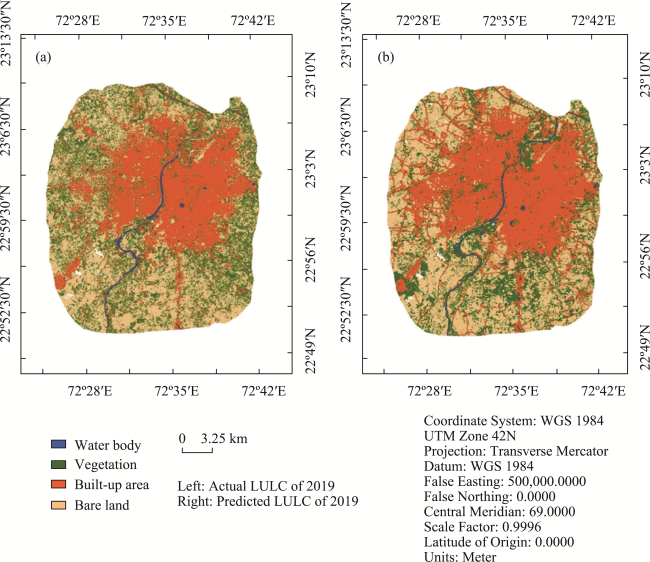
Table 6 LULC-predicted versus actual value for the year 2019
LU Class Actual area (km2) Predicted area (km2) Percentage difference
Water body 11.24 11.83 -5.24
Vegetation 226.60 189.11 -16.55
Built-up area 305.24 330.99 8.44
Others 357.47 368.62 3.12
Figure 6 Actual and predicted LULC map of Ahmedabad in 2019
Figure 7 The various urban growth drivers selected for predicting Ahmedabad’s 2030 urban growth
By 2030, the Built-up LU class area is expected to undergo the largest change of 31.45%, rising from 305 km2 to 383 km2 (refer to Figure 8 and Table 7). Most of this increase in the city’s built-up area shall be compensated by a decline in the “Others” geographical spread. Overall, the available open grounds, bare lands, uncropped agricultural areas shall reduce from 358 km2 in 2019 to 271 km2 by 2030. The city’s green cover shall grow slightly from 227 km2 in 2019 to 234 km2 in 2030. No appreciable changes are expected in the size and locations of the city’s water bodies. Besides, as per regression estimates, the city's population is expected to grow by 18.8%, reaching 93.5 lakhs in 2030 from 78.70 lakhs in 2019. As per the equation in Figure 6, a 93.5 lakh population in 2030 shall require a 374.2 km2 of built-up area close to 383.29 km2 predicted by the future LULC map. In the absence of sophisticated LULC modelling tools, this equation can be adopted for predicting future urban expansion in this region.
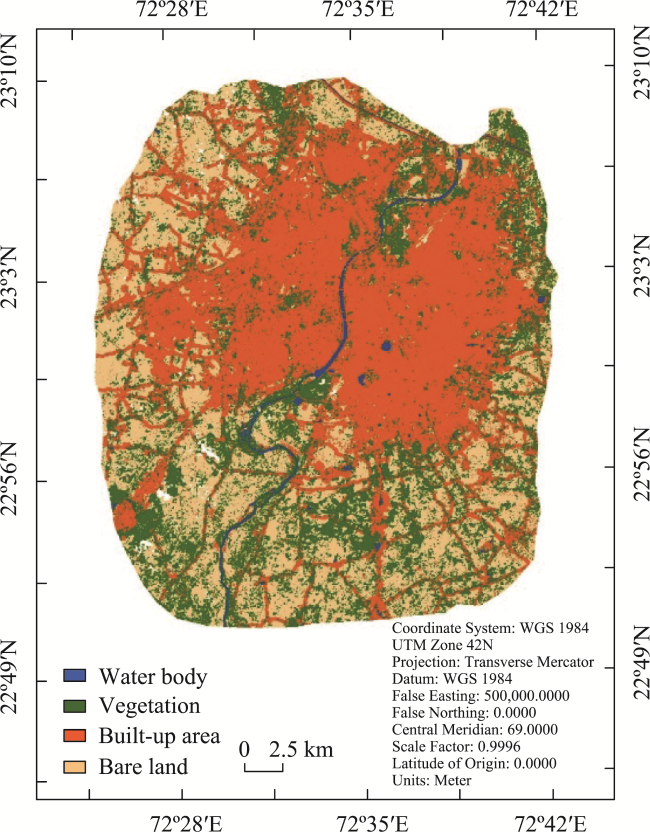
Figure 8 Ahmedabad predicted LULC map in 2030
Table 7 Area under each LU class (km2) in 2019 and 2030
LU class 2019 2030
Water body 11.24 11.78
Vegetation 226.60 234.24
Built-up area 305.24 383.29
Others 357.47 271.25
Between 1990 to 2019, Ahmedabad witnessed massive urban development at the expense of forests, bare lands, cultivable and un-cropped farmlands. In this period, the total built-up area grew from 145 km2 to 305 km2. During 1990-2000, most residential developments focused westward of the Sabarmati river along Chandlodia, Vijaynagar, Ramdevnagar and Parvati Nagar. On the river’s eastward side, residential development focused on Hansol, Sardarnagar and Sukharamnagar. The industrial growth was concentrated around Naroda and Odhav. Most new developments followed the city’s main transportation routes, infilling around existing developed areas. The fastest urban expansion occurred between 2000-2010. In 2010, Forbes magazine placed Ahmedabad as the third-fastest growing city globally (DNA, 2010). Rapid industrial growth and job opportunities attracted people from different parts of the state and country. Large scale urban (residential and commercial) development trailed Chandkheda and Ranip in the North and Thaltej, Sarkhej, Changodar and Bopal in the South. The development of new roads and civic infrastructure also attracted people to occupy outer semi-urban and sub-urban areas encouraging further expansion. Further, 25.6% of the city’s population lived in slums and informal settlements in 1990. This figure fell to 4.5% in 2011 due to better work opportunities and Ahmedabad’s municipal corporation’s slum-housing and networking project (Bhatt 2003; Wikipedia 2021a). During 2010-2019, several manufacturing, pharmaceuticals and information technology companies opened along the Thaltej-Sarkhej highway in the city’s south. The economic sector also benefitted from the expansion and re-development of the city’s international airport. The eastern industrial belt along Kathwada, Naroda, Chiloda, and Odhav has expanded further.
Besides many socio-economic benefits, Ahmedabad’s rapid urbanization has produced several unintended consequences. Rapid urbanization infilling around developed areas increased urban density in older city areas. The higher urban density restricts local administration ability to provide necessary health and sanitation facilities to city dwellers creating several social and health challenges. For instance, urban slums face higher vulnerability to heatwaves, floods and shortage of potable water. Due to faster transmission rates, the densely urbanized regions are hit hardest during pandemics. Next, the outward urban expansion beyond existing city boundaries has destroyed many bare and agricultural lands. Initially, most farmlands get encroached by low-density urban development, and gradually these sparsely-populated areas become high-density zones due to rising industrial, residential, and business activities. The higher market value of agricultural lands near urban areas encourages farmers to sell their lands for urban development. Relaxed land-use laws allowing fragmentation of farmlands also harm surrounding farms’ physical and chemical properties. Noteworthy, the decline in agricultural lands size and productivity threatens regional food security for the future.
Further, between 1990-2019, most areas have shifted towards higher LST. Prevailing trends suggest substantial increments of 18.8% and 31.45% to the city’s population and urban extents by 2030. Thus, there is a looming need to develop sustainable urban development policies to balance future growth and environmental harm. Sustainable policies must decrease forests and cultivate land exploitation, consolidation and reclamation. Tax, loan preferences and financial subsidies should be given to companies having low land demands, and high capital taxes can be imposed on low land output efficiency and poor land use. Decentralized urban spaces (e.g. satellite towns) can reduce urban density and prevent large UHI zones in the future. Further, large-scale urban greening measures can also limit UHI effects.

5 Conclusions

This study performed a spatio-temporal assessment of Ahmedabad’s urban growth during the past three decades (1990-2019). The Maximum Likelihood Algorithm classified four (1990, 2000, 2010, 2019) coarse resolution (30 m × 30 m) satellite images into Built-up, Vegetation, Water body and “Others” land-use (LU) classes. During 1990-2019, the city’s urban area grew substantially in extent and density from 132 km2 in 1990 to 305 km2 in 2019. Urbanization engulfed large swaths of open spaces, bare lands, and uncultivated farms, plummeting total “Others” LU area from 641 km2 in 1990 to 357 km2 in 2019. The green cover grew moderately from 161 km2 in 1990 to 227 km2 during 2019, and water bodies did not show much fluctuation. New urban development appears to follow the main transportation routes, infilling and expanding existing developed areas.
A rapidly rising population is the primary driver for Ahmedabad’s fast urban growth. The city is adding almost 3.9 km2 additional built-up space to accommodate every 1 lakh (100,000) new residents into the city. Rising urban density stresses the city’s infrastructure, hampering the supply of essential services like housing, health and sanitation. Moreover, the destruction of open spaces and farmlands for new development has reduced food production and increased urban heating. The application of an MLP-MCA model predicts a 25% increase in Ahmedabad’s total urban area up to 383 km2 in 2030. In comparison, the “Others” LU class area is expected to fall by 24% to 271 km2. Moreover, the city’s population is expected to swell by 19%, from 78.70 lakhs in 2019 to 93.5 lakhs in 2030. Unchanged, these trends shall give rise to several socio-economic and environmental problems.
Future urban development policies must balance further development and environmental damage. A strong commitment and coordination is necessary between different government agencies to strictly implement land laws. Financial incentives for industries displaying high levels of land output efficiency and strict penalties on illegal land encroachments should be imposed. Urban greening such as parks, lakes and sustainable building construction can also help reduce UHIs. Notably, this study used past urban growth trends to develop future predictions. Several advanced modelling techniques can also predict future development based on alternative urban development theories. Thus, follow up studies should predict Ahmedabad’s urban growth under “Environmentally Conscious”, “Business as Usual” and “Environmentally Wasteful” scenarios.

The authors would like to acknowledge the funding received from the Department of Science and Technology, Government of India (DST/TMD/UKBEE/2017/17). Projects: Zero Peak Energy Demand for India (ZED-I) and Engineering and Physics Research Council EPSRC (EP/R008612/1).

[1]
Abd EL-kawy O R et al., 2019. Temporal detection and prediction of agricultural land consumption by urbanization using remote sensing. Egyptian Journal of Remote Sensing and Space Science, 22(3): 237-246. doi: 10.1016/j.ejrs.2019.05.001.

DOI

[2]
Ahmad F, Goparaju L, Qayum A, 2017. LULC analysis of urban spaces using Markov chain predictive model at Ranchi in India. Spatial Information Research, 25(3): 351-359. doi: 10.1007/s41324-017-0102-x.

DOI

[3]
Ahmed B et al., 2013. Simulating land cover changes and their impacts on land surface temperature in Dhaka, Bangladesh. Remote Sensing, 5(11): 5969-5998. doi: 10.3390/rs5115969.

DOI

[4]
Ahmed B, Ahmed R, 2012. Modeling urban land cover growth dynamics using multioral satellite images: A case study of Dhaka, Bangladesh. ISPRS International Journal of Geo-Information, 1(1): 3-31. doi: 10.3390/ ijgi1010003.

DOI

[5]
Alqurashi A F, Kumar L, 2014. Land use and land cover change detection in the Saudi Arabian desert cities of Makkah and Al-Taif using satellite data. Advances in Remote Sensing, 3(3): 106-119. doi: 10.4236/ars.2014. 33009.

DOI

[6]
Araya Y H, Cabral P, 2010. Analysis and modeling of urban land cover change in Setúbal and Sesimbra, Portugal. Remote Sensing, 2(6): 1549-1563. doi: 10.3390/rs2061549.

DOI

[7]
Arulbalaji P, 2019. Analysis of land use land cover changes using geospatial techniques in Salem district, Tamil Nadu, South India. SN Applied Sciences, 1(5). doi: 10.1007/s42452-019-0485-5.

DOI

[8]
Atkinson P M, Tatnall A R L, 1997. Introduction neural networks in remote sensing. International Journal of Remote Sensing, 18(4): 699-709. doi: 10.1080/014311697218700.

DOI

[9]
Baby S, 2015. Monitoring the coastal land use land cover changes (LULCC) of Kuwait from spaceborne LANDSAT sensors. Indian Journal of Geo-Marine Sciences (IJMS), 44(6): 927-932.

[10]
Belal A A, Moghanm F S, 2011. Detecting urban growth using remote sensing and GIS techniques in Al Gharbiya governorate, Egypt. Egyptian Journal of Remote Sensing and Space Science, 14(2): 73-79. doi: 10.1016/j.ejrs.2011.09.001.

DOI

[11]
Bhatt M, 2003. Case studies for the Global Report on Human Settlements:Ahmedabad, India: 1-23.Available at: https://www.ucl.ac.uk/dpu-projects/Global_Report/pdfs/Ahmedabad_bw.pdf

[12]
Bhugeloo A et al., 2019. Tracking indigenous forest cover within an urban matrix through land use analysis: The case of a rapidly developing African city. Remote Sensing Applications: Society and Environment, 13(December 2018): 328-336. doi: 10.1016/j.rsase.2018.12.003.

DOI

[13]
Borbora J, Das A K, 2014. Summertime Urban Heat Island study for Guwahati City, India. Sustainable Cities and Society, 11: 61-66. doi: 10.1016/j.scs.2013.12.001.

DOI

[14]
Chang-Martínez L A et al., 2015. Modeling historical land cover and land use: A review from contemporary modeling. ISPRS International Journal of Geo-Information, 4(4): 1791-1812. doi: 10.3390/ijgi4041791.

DOI

[15]
Congalton R G, Green K, 2019. Assessing the Accuracy of Remotely Sensed Data: Principles and Practices. The CRC Press.

[16]
Dewan A M, Yamaguchi Y, 2009. Land use and land cover change in Greater Dhaka, Bangladesh: Using remote sensing to promote sustainable urbanization. Applied Geography, 29(3): 390-401. doi: 10.1016/j.apgeog. 2008.12.005.

DOI

[17]
DNA, 2010. Cheers Ahmedabad! City is racing ahead. Available at: https://www.dnaindia.com/india/report-cheers-ahmedabad-city-is-racing-ahead-1453361Accessed: May 18, 2021).

[18]
Eastman J, 2009. IDRISI Taiga: Guide to GIS and Image Processing Volume: Manual version 16.02. (August): 325.

[19]
GeoKnowledge, 2020. Image Processing for ERDAS | Learning Materials.Available at: http://learningzone.rspsoc.org.uk/index.php/Learning-Materials/Image-Processing-for-ERDAS/6.1.-IntroductionAccessed: 20 May 2021).

[20]
Gohain K J, Mohammad P, Goswami A, 2021. Assessing the impact of land use land cover changes on land surface temperature over Pune city, India. Quaternary International, 575, 259-269. doi: 10.1016/j.quaint.2020.04.052.

DOI

[21]
Gupta M et al., 2021. Transmission dynamics of the COVID-19 epidemic in India and modeling optimal lockdown exit strategies. International Journal of Infectious Diseases, 103: 579-589. doi: 10.1016/j.ijid.2020.11.206.

DOI PMID

[22]
Haklay M, Weber P, 2008. OpenStreet map: User-generated street maps. IEEE Pervasive Computing, 7(4): 12-18. doi: 10.1109/MPRV.2008.80.

DOI

[23]
Han H, Yang C, Song J, 2015. Scenario simulation and the prediction of land use and land cover change in Beijing, China. Sustainability (Switzerland), 7(4): 4260-4279. doi: 10.3390/su7044260.

DOI

[24]
Hassan Z et al., 2016. Dynamics of land use and land cover change (LULCC) using geospatial techniques: A case study of Islamabad Pakistan. SpringerPlus, 5(1). doi: 10.1186/s40064-016-2414-z.

DOI

[25]
Hegazy I R, Kaloop M R, 2015. Monitoring urban growth and land use change detection with GIS and remote sensing techniques in Daqahlia governorate Egypt. International Journal of Sustainable Built Environment, 4(1): 117-124. doi: 10.1016/j.ijsbe.2015.02.005.

DOI

[26]
Herold M et al., 2006. Evolving standards in land cover characterization. Journal of Land Use Science, 1(2-4): 157-168. doi: 10.1080/17474230601079316.

DOI

[27]
Islam M A, Dinar Y, 2021. Evaluation and spatial analysis of road accidents in Bangladesh: An emerging and alarming issue. Transportation in Developing Economies, 7(1): 1-14. doi: 10.1007/s40890-021-00118-3.

DOI

[28]
Kaliraj S et al., 2017. Coastal landuse and land cover change and transformations of Kanyakumari coast, India using remote sensing and GIS. Egyptian Journal of Remote Sensing and Space Science, 20(2): 169-185. doi: 10.1016/j.ejrs.2017.04.003.

DOI

[29]
Kookana R S et al., 2020. Urbanisation and emerging economies: Issues and potential solutions for water and food security. Science of the Total Environment, 732: 139057. doi: 10.1016/j.scitotenv.2020.139057.

DOI

[30]
Kuddus M A, Tynan E, McBryde E, 2020. Urbanization: A problem for the rich and the poor? Public Health Reviews, 41(1): 1-4. doi: 10.1186/s40985-019-0116-0.

DOI

[31]
Losiri C et al., 2016. Modeling urban expansion in Bangkok Metropolitan region using demographic-economic data through cellular Automata-Markov Chain and Multi-Layer Perceptron-Markov Chain models. Sustainability (Switzerland), 8(7). doi: 10.3390/su8070686.

DOI

[32]
Mahadevia D, Desai R, Vyas S, 2014. City Profile: Ahmedabad Darshini. Centre for Urban Equity - Working Paper Series,74. Available at: https://cept.ac.in/UserFiles/File/CUE/WorkingPapers/RevisedNew/26CUEWP26_CityProfileAhmedabad.pdf

[33]
Mansour S, Al-Belushi M, Al-Awadhi T, 2020. Monitoring land use and land cover changes in the mountainous cities of Oman using GIS and CA-Markov modelling techniques. Land Use Policy, 91(June 2019):104414. doi: 10.1016/j.landusepol.2019.104414.

DOI

[34]
Meshesha T W, Tripathi S K, Khare D, 2016. Analyses of land use and land cover change dynamics using GIS and remote sensing during 1984 and 2015 in the Beressa Watershed Northern Central Highland of Ethiopia. Modeling Earth Systems and Environment, 2(4). doi: 10.1007/s40808-016-0233-4.

DOI

[35]
Mishra V N, Rai P K, 2016. A remote sensing aided multi-layer perceptron: Markov chain analysis for land use and land cover change prediction in Patna district (Bihar), India. Arabian Journal of Geosciences, 9(4). doi: 10.1007/s12517-015-2138-3.

DOI

[36]
Mohamed A, Worku H, 2020. Simulating urban land use and cover dynamics using cellular automata and Markov chain approach in Addis Ababa and the surrounding. Urban Climate, 31(October 2019):100545. doi: 10.1016/j.uclim.2019.100545.

DOI

[37]
MohanRajan S N, Loganathan A, Manoharan P, 2020. Survey on Land use land cover (LULC) change analysis in remote sensing and GIS environment: Techniques and challenges. Environmental Science and Pollution Research, 27(24): 29900-29926. doi: 10.1007/s11356-020-09091-7.

DOI

[38]
Nurwanda A, Honjo T, 2020. The prediction of city expansion and land surface temperature in Bogor City, Indonesia. Sustainable Cities and Society, 52(December 2018):101772. doi: 10.1016/j.scs.2019.101772.

DOI

[39]
Nwaogu C, Benc A, Pechanec V, 2017. Prediction models for landscape development in GIS. In: Proceedings of GIS Ostrava, 289-304. doi: 10.1007/978-3-319-61297-3.289304.

DOI

[40]
Pal S, Ziaul S, 2017. Detection of land use and land cover change and land surface temperature in English Bazar urban centre. Egyptian Journal of Remote Sensing and Space Science, 20(1): 125-145. doi: 10.1016/j.ejrs. 2016.11.003.

DOI

[41]
Power A L et al., 2018. Monitoring impacts of urbanisation and industrialisation on air quality in the Anthropocene using urban pond sediments. Frontiers in Earth Science, 6: 131. doi: 10.3389/feart.2018.00131.

DOI

[42]
Rahman M T, 2016. Detection of land use land cover changes and urban sprawl in Al-Khobar, Saudi Arabia: An analysis of multi-temporal remote sensing data. ISPRS International Journal of Geo-Information, 5(2). doi: 10.3390/ijgi5020015.

DOI

[43]
Rahman M T, Aldosary A S, Mortoja M G, 2017. Modeling future land cover changes and their effects on the land surface temperatures in the Saudi Arabian eastern coastal city of Dammam. Land, 6(2). doi: 10.3390/land6020036.

DOI

[44]
Rawat J S, Biswas V, Kumar M, 2013. Changes in land use/cover using geospatial techniques: A case study of Ramnagar town area, district Nainital, Uttarakhand, India. Egyptian Journal of Remote Sensing and Space Science, 16(1): 111-117. doi: 10.1016/j.ejrs.2013.04.002.

DOI

[45]
Saravanan V S et al., 2016. Urbanization and human health in urban India: Institutional analysis of water-borne diseases in Ahmedabad. Health Policy and Planning, 31(8): 1089-1099. doi: 10.1093/heapol/czw039.

DOI PMID

[46]
Seitzinger S P et al., 2015. International Geosphere-Biosphere Programme and Earth system science: Three decades of co-evolution. Anthropocene, 12(2015): 3-16. doi: 10.1016/j.ancene.2016.01.001.

DOI

[47]
Shafizadeh Moghadam H, Helbich M, 2013. Spatiotemporal urbanization processes in the megacity of Mumbai, India: A Markov chains-cellular automata urban growth model. Applied Geography, 40: 140-149. doi: 10.1016/j.apgeog.2013.01.009.

DOI

[48]
Al shawabkeh R et al., 2019. The role of land use change in developing city spatial models in Jordan: The case of the Irbid master plan (1970-2017). Alexandria Engineering Journal, 58(3). doi: 10.1016/j.aej.2019.08.001.

DOI

[49]
Shi K et al., 2016. Urban expansion and agricultural land loss in China: A multiscale perspective. Sustainability (Switzerland), 8(8): 1-16. doi: 10.3390/su8080790.

DOI

[50]
Shukla A, Jain K, 2019. Modeling urban growth trajectories and spatiotemporal pattern: A case study of Lucknow City, India. Journal of the Indian Society of Remote Sensing, 47(1): 139-152. doi: 10.1007/s12524-018- 0880-1.

DOI

[51]
Silva L P E et al., 2020. Modeling land cover change based on an artificial neural network for a semiarid river basin in northeastern Brazil. Global Ecology and Conservation, 21: e00811. doi: 10.1016/j.gecco.2019.e00811.

DOI

[52]
Sultana S, Satyanarayana A N V, 2020. Assessment of urbanisation and urban heat island intensities using landsat imageries during 2000-2018 over a sub-tropical Indian city. Sustainable Cities and Society, 52(September 2019): 101846. doi: 10.1016/j.scs.2019.101846.

DOI

[53]
Suribabu, C. R., Bhaskar, J. and and Neelakantan, T. R. 2012. Land use/cover change detection of Tiruchirapalli City, India, using integrated remote sensing and GIS tools. Journal of the Indian Society of Remote Sensing, 40(4): 699-708. doi: 10.1007/s12524-011-0196-x.

DOI

[54]
Tahir M, Imam E. Hussain T, 2013. Evaluation of land use land cover changes in Mekelle City, Ethiopia using Remote Sensing and GIS. Computational Ecology and Software, 3(1): 9-16.

[55]
Tarawally M et al., 2019. Land use land cover change evaluation using land change modeller: A comparative analysis between two main cities in Sierra Leone. Remote Sensing Applications: Society and Environment, 16(February): 100262. doi: 10.1016/j.rsase.2019.100262.

DOI

[56]
Tripathi D K, Kumar M, 2012. Remote sensing based analysis of land use/land cover dynamics in Takula Block, Almora District (Uttarakhand). Journal of Human Ecology, 38(3): 207-212. doi: 10.1080/09709274.2012. 11906489.

DOI

[57]
Usman M et al., 2015. Land use land cover classification and its change detection using multi-temporal MODIS NDVI data. Journal of Geographical Sciences, 25(12): 1479-1506. doi: 10.1007/s11442-015-1247-y.

DOI

[58]
Vermeulen L C et al., 2015. Modelling the impact of sanitation, population growth and urbanization on human emissions of Cryptosporidium to surface waters: A case study for Bangladesh and India. Environmental Research Letters, 10(9). doi: 10.1088/1748-9326/10/9/094017.

DOI

[59]
Wakode H B et al., 2014. Analysis of urban growth using Landsat TM/ETM data and GIS: A case study of Hyderabad, India. Arabian Journal of Geosciences, 7(1): 109-121. doi: 10.1007/s12517-013-0843-3.

DOI

[60]
Welsh P, 2004. Urban future. Highways, 74(2): 47-48. doi: 10.4324/9781315652597-13.

DOI

[61]
Wikipedia, 2021a. Ahmedabad - Wikipedia.Available at: https://en.wikipedia.org/wiki/AhmedabadAccessed: May 18, 2021).

[62]
Wikipedia, 2021b. Geography of Ahmedabad.Available at: https://en.wikipedia.org/wiki/Geography_of_AhmedabadAccessed: 21 May 2021).

[63]
Wikipedia, 2021c. Landsat program.Available at: https://en.wikipedia.org/wiki/Landsat_programAccessed: 21 May 2021).

[64]
Wikipedia, 2021d. List of largest cities.Available at: https://en.wikipedia.org/wiki/List_of_largest_cities#ListAccessed: 22 May 2021).

[65]
World Population Review, 2021. Ahmedabad Population 2021 (Demographics, Maps, Graphs).Available at: https://worldpopulationreview.com/en/world-cities/ahmedabad-populationAccessed: 18 May 2021).

[66]
Zhu H M, You W H, Zeng Z fa, 2012. Urbanization and CO2 emissions: A semi-parametric panel data analysis. Economics Letters, 117(3): 848-850. doi: 10.1016/j.econlet.2012.09.001.

DOI

Outlines

/