Original article

Exploring spatial relationships between stream channel features, water depths and flow velocities during flash floods using HEC-GeoRAS and Geographic Information Systems

  • Miguel LEAL , 1, 2 ,
  • Eusébio REIS 1 ,
  • Pedro Pinto SANTOS 1
Expand
  • 1. Centre of Geographical Studies and Associated Laboratory TERRA, Institute of Geography and Spatial Planning, Universidade de Lisboa. Edifício IGOT, Rua Branca Edmée Marques, 1600-276 Lisbon, Portugal
  • 2. Forest Research Centre and Associated Laboratory TERRA, School of Agriculture, Universidade de Lisboa. Tapada da Ajuda, 1349-017 Lisbon, Portugal

Miguel Leal (1988-), PhD, specialized in flooding and risk analysis. E-mail:

Received date: 2021-05-26

  Accepted date: 2021-10-20

  Online published: 2022-06-25

Supported by

Centre of Geographical Studies(No.UIDB/00295/2020)

Centre of Geographical Studies(No.UIDP/00295/2020)

FCT-Portuguese Foundation for Science and Technology, I.P.(No.SFRH/BD/96632/2013)

FCT-Portuguese Foundation for Science and Technology, I.P.(No.CEEIND/00268/2017)

Project BeSafeSlide(No.PTDC/GES-AMB/30052/2017)

Abstract

Water depths and flow velocities decisively influence the damage caused by flash floods. Geographic Information System (GIS) is a powerful and useful tool, allowing the spatial analysis of results obtained by hydraulic modelling, namely from the HEC-RAS/HEC- GeoRAS software. The GIS spatial analysis performed in this study seeks to explain and quantify the spatial relationships between the stream channel features and flow components during flash flood events. Despite these relationships are generically known, there are few studies exploring this subject in different geographic contexts. A 1D hydraulic model was applied in a small watershed in Portugal, providing good results in the definition of floodable areas, water depths and longitudinal velocities. No direct relationship was found between water depths and velocities in the floodable areas; however, negative strong correlations were found between the two flow components along the stream centerlines. Bed slope, channel and flood width, and roughness prove to be highly relevant on the longitudinal variations of water depths and velocities and on the location of maximum values. Increasing peak discharges and return periods (RT) can change the relationships between water depths and velocities at the same location. Results can be improved with more accurate elevation data for stream channels and floodplains.

Cite this article

Miguel LEAL , Eusébio REIS , Pedro Pinto SANTOS . Exploring spatial relationships between stream channel features, water depths and flow velocities during flash floods using HEC-GeoRAS and Geographic Information Systems[J]. Journal of Geographical Sciences, 2022 , 32(4) : 757 -782 . DOI: 10.1007/s11442-022-1971-z

1 Introduction

The intensity of a flood can be measured by water depths, flow velocities, duration of the flood event, amount of solid load, or concentration of pollutants, and these characteristics influence the extent of the damage caused by this natural hazard (Merz et al., 2007). Water depth is generally the most used variable in flood risk assessments (Penning-Rowsell et al., 2005; Middelmann-Fernandes, 2010; de Moel et al., 2015) because the energy head, i.e., the total energy according to the Bernoulli equation, is mostly governed by this variable (Kreibich et al., 2009). Furthermore, flood stage determines the extent of the flooded areas, the affected elements and whether the floodwaters reach the openings of the exposed buildings, making it difficult to assist and evacuate people. Specifically for flash floods, water depth and flow velocity should be used together in hazard and risk assessments (Penning- Rowsell et al., 2005, Zimmermann et al., 2005, Merz et al., 2007, Kreibich et al., 2009, Asano and Uchida, 2016). Both variables are fundamental for the stability of people and vehicles in floodwaters (e.g., Abt et al., 1989; Karvonen et al., 2000; Jonkman and Penning-Rowsell, 2008; Jonkman and Vrijling, 2008; Xia et al., 2011, 2014; Kvočka et al., 2016; Arrighi et al., 2017) and for structural damage in buildings and infrastructures (Smith, 1991; Soetanto and Proverbs, 2004; Thieken et al., 2005; Merz et al., 2010; Middelmann- Fernandes, 2010; Hammond et al., 2015).
The floodable areas, water depths and flow velocities associated to different return periods are usually the result of flood hazard assessments using hydraulic modelling (e.g., Penning-Rowsell et al., 2005; Zimmermann et al., 2005; Merz et al., 2007; Kvočka et al., 2016; Ţîncu et al., 2018). This is also used to describe the flow behavior in river channels with different morphologies during average or high-magnitude discharges (e.g., Ottevanger et al., 2012; Mohanty et al., 2014; Gholami et al., 2015; Harrison et al., 2015; Pradhan et al., 2018; Mirauda and Russo, 2019), to perform sensitivity analyses or to calibrate the parameters and variables with influence on the results provided by different software (e.g., Horritt and Bates, 2002; Pappenberger et al., 2006; Aronica et al., 2012; Balica et al., 2013; Geravand et al., 2020). However, most of the hydraulic models cannot fully capture and explain the complexity of the flow behavior in river channels and floodplains, especially with respect to the distribution of velocities in meandering channels (Shao et al., 2003; Patra et al., 2004; Ottevanger et al., 2012; Liu et al., 2014; Mohanty et al., 2014). Bed slope, channel and floodplain roughness, water depth, channel and floodplain width, and radius curvatures in river bends control the flow velocity (Mudd, 2006, Blanckaert and de Vriend, 2010; Crispino et al., 2015; Biscarini et al., 2016; Xing et al., 2016). The estimation of the longitudinal, lateral and vertical velocities has been a recurrent topic of research (Patra et al., 2004; Marini et al., 2011; Fontana et al., 2013; Song et al., 2017), but the results obtained are difficult to validate for flash flood events (Moramarco et al., 2011; Asano and Uchida, 2016; Chen et al., 2020).
Despite the spatial relationships between water depths and flow velocities and the influence of channel features on these flow components are generically known, there are few studies exploring this subject for flash floods in different geographic contexts (Kreibich et al., 2009; Zhang et al., 2009; Asano and Uchida, 2016; Xing et al., 2016; Chen et al., 2020). The temporal and spatial changes in water depth and flow velocity are complex (Asano and Uchida, 2016), but it is essential to improve the knowledge on flow behavior during high-magnitude events. The research on flash floods usually follows one of two different perspectives: the engineering perspective, directed to the hydrologic and hydraulic modelling, and the hazard/risk perspective, focused on the damage caused by natural hazards. This work seeks to connect these two viewpoints using a geographical perspective and Geographic Information Systems (GIS), which allow both the spatial representation of the results from hydraulic modelling and the spatial analysis on flow components and channel features (Khatami and Khazaei, 2014; Elkhrachy, 2015). Despite GIS are frequently used to map flood occurrences and flow components, and to assess flood hazard/risk (e.g., Meyer et al., 2009; Diakakis et al., 2016; Santos and Reis, 2017), there is no scientific tradition to apply their potential to perform a local scale spatial and statistical analysis to flow components and their conditioning factors.
In this study, hydraulic modelling was performed using HEC-RAS and HEC-GeoRAS for ArcMap and was applied to a small ungauged watershed near Lisbon (Portugal), which has an important historical record of human and material damage in the last decades. Spatial analysis on the floodable areas, water depths and flow velocities for several return periods were performed to detect how these flow components are spatially interrelated and are affected by the stream channel features. The main goals of this study are: 1) to quantify spatial relationships between water depths and flow velocities resorting to HEC-GeoRAS, evidencing the usefulness of GIS on this field of knowledge; 2) to demonstrate how the magnitude of flash flood events can change the flow spatial patterns/dynamics and the location of the highest values of water depth and flow velocity; and 3) to estimate the effects of stream channel features (geometry, bed slope, roughness) on flow components.

2 Study area

Barcarena is a small, elongated watershed (area of 34.2 km2 and a form factor of 0.2) close to the Portuguese capital (Lisbon) and included in the municipalities of Sintra and Oeiras (Figure 1). The main watercourse is a 4th order stream (Strahler classification) of 19.4 km long, which flows into the Tagus River, near the Atlantic Ocean. The time of concentration (according to the Temez method) and the lag time for this watershed are, respectively, 6h20m and 3h48m. Elevation ranges between mean sea level and 330 m. Overland flow is favored by low-permeability bedrock (marls, limestones and basalts) and soils (predominantly clayey), and by the widespread of impervious surfaces. Almost half of its area is built-up. There were 26 occurrences with important human and material damage reported in newspapers and insurance claims caused by flash floods during the 20th and the 21st centuries in the Barcarena watershed. The most destructive event occurred in November 1967, when hundreds of lives were lost in the Lisbon Metropolitan Area as a result of flash floods (Ramos and Reis, 2001, 2002; Trigo et al., 2016; Leal et al., 2018), causing 8 fatalities in this watershed.
The study area is in the middle section of this watershed, including about 1000 m of the Barcarena stream and the last 350 m of the Massamá stream, one of its main tributaries (Figure 1). In the study area, the average bed slopes are 1.9% for the Barcarena stream and 6% for the Massamá stream. Channels are narrow, not exceeding 15 m in the widest sector. Manning’s roughness coefficients range between 0.02 and 0.04 along the stream channels and between 0.02 and 0.07 in the floodplains. The confluence of the Barcarena and the Massamá streams is a critical point defined by the National Laboratory for Civil Engineering (LNEC). Flash floods in this area are recurrent and even low return period events can damage exposed buildings. Retaining stone walls were built in some parts of this section to prevent lateral erosion and/or flooding. In November 2011, the most recent damaging event, retaining walls and a pedestrian bridge near the confluence of the Barcarena and Massamá streams were destroyed, and floodwaters entered the houses. Important human and material damage were also reported in the study area during the high-magnitude events of November 1967 and February 2008 (Leal, 2019; Leal et al., 2019).
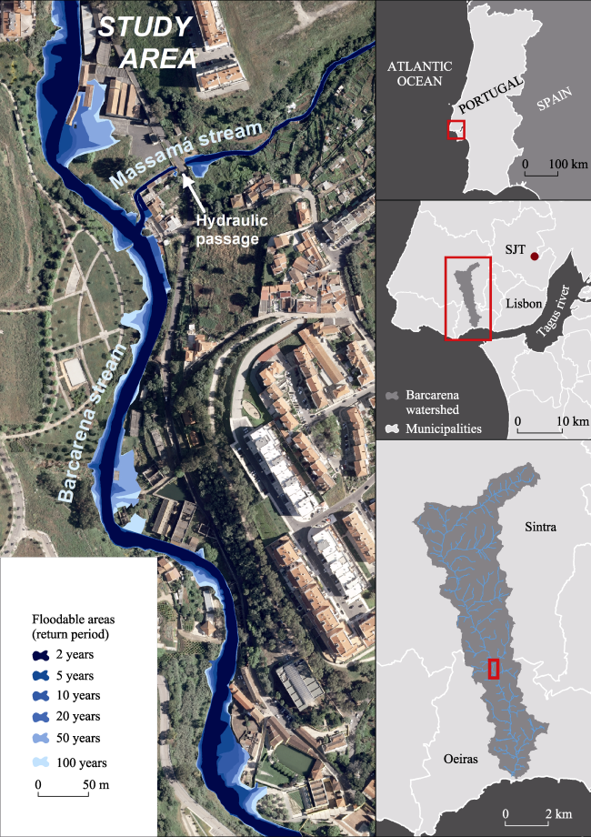
Figure 1 Location of the study area in the Barcarena watershed and the floodable areas for the n-year RT

3 Data and methods

3.1 Hydrologic modelling

There are no hydrometric data for the Barcarena watershed. For this reason, peak discharges for the return periods (RT) of 2, 5, 10, 20, 50 and 100 years were obtained using designed hyetographs and a rainfall-runoff model performed in HEC-HMS software (Figure 2). The designed hyetographs for the considered return periods were developed from the IDF (intensity-duration-frequency) curves of the São Julião do Tojal (SJT in Figure 1), a rain gauge located about 15 km NE to the study area. The IDF curves were built from the parameters available in Brandão et al. (2001), which was established from a period with 34 years of data (equation 1):
i(d,Rt)=a.(db)
where i(d,Rt) is the rainfall intensity i (mm) associated with a given d duration (min) and Rt return period (years); a and b are parameters resulting from the adjustment between rainfall intensities and durations (associated with a given return period) by the least-squares method.
The hyetographs were designed using the alternating block method and are composed by blocks of 10 minutes. The alternating block hyetograph (Chow et al., 1988) is one of the methods based on the IDF curves, as the Chicago hyetograph (Keifer and Chu, 1957). These methods produce the highest peak flows, resulting in critical flood situations and reliable design values, but are not intended to represent real event patterns (Grimaldi et al., 2012; Sordo-Ward et al., 2014; Na and Yoo, 2018; Chimene and Campos, 2020). The duration of the estimated storms equals the time of concentration of the Barcarena watershed. The Soil Conservation Service curve number (SCS-CN) for AMC III (antecedent moisture conditions -saturated soils) was chosen as the loss method and lag time as the transform method in HEC-HMS.
The peak discharges were obtained for the Barcarena and Massamá streams. For the Barcarena stream, peak discharges were estimated upstream and downstream of the confluence with the Massamá stream. Later, these values were inserted in HEC-RAS software for hydraulic modelling (Figure 2).

3.2 Digital Surface Model (DSM)

The quality of a Digital Surface Model (DSM) is affected by the spatial distribution, density and accuracy of the elevation data, the spatial resolution of the model and the interpolation methods (Hutchinson and Gallant, 2000; Zhang et al., 2016; Habib et al., 2020). The first version of the DSM for the study area was built in GIS (ArcMap software) using elevation data (contour lines and elevation points) at 1:2000 scale provided by the Oeiras City Hall. However, and despite the detailed scale, there is no elevation data along the stream channels, except when crossed by the contour lines, creating flat areas upstream and downstream this point, separated by a 2-m step. This will be an obvious misrepresentation of the channel’s morphology and of its longitudinal variation in the DSM, leading to consequent errors in the floodable areas, water depths and flow velocities. These weaknesses can be eliminated by creating a “hydrologically correct” DSM from the Topo to Raster tool of ArcMap. This allows the insertion of the location of the thalwegs in the DSM, i.e., the line of the lowest elevation in the stream bed, ensuring the transversal and longitudinal variations in elevation along the stream channels. Buildings were also included in the DSM as polygons with higher elevations than the surrounding areas to estimate their effects on the floodable areas, water depths and flow velocities. The survey and vectorization of the buildings were performed using orthophotos (resolution of 10 cm) provided by the Oeiras City Hall. The final DSM includes contour lines, elevation points, buildings and the position of the thalwegs (Figure 2). The correctness and accuracy of the DSM is essential for the quality of the hydraulic modelling results (Horritt and Bates, 2002; Werner, 2004; Merz et al., 2007; Lastra et al., 2008).

3.3 Hydraulic modelling and spatial analysis

Hydraulic modelling was performed through the interconnection between HEC-RAS and HEC-GeoRAS for ArcMap in three steps: pre-processing, modelling and post-processing (Geravand et al., 2020). In the first step, stream centerlines, bank lines, flow path centerlines, cross-sections (XS cut lines) and the Manning’s roughness coefficients (Chow et al., 1988) for channels and floodplains were defined with HEC-GeoRAS using the DSM, according to the orientations of USACE (2009). Cross-sections were drawn perpendicularly to the streamlines and separated by 10 m, in average. Cross-sections were placed closer in confluences, bends or natural/artificial narrowing of the stream channels to capture changes in their geometry and morphology.
The input data generated in HEC-GeoRAS and the peak discharges obtained in HEC-HMS (Figure 2) were imported to HEC-RAS for modelling (second step). Peak discharges were used to determine steady flow water surface profiles for the 2-, 5-, 10-, 20-, 50- and 100-year RT along the study area. In steady-state condition, water surface elevation and flow velocity were calculated by HEC-RAS for each discrete cross-section by solving continuity, energy and roughness (Manning) equations (Cook and Merwade, 2009). Mixed flow regime and the boundary condition normal depth slope were chosen for the HEC-RAS computation. There is only one infrastructure in the study area that is relevant to be included in hydraulic modelling: a hydraulic passage/culvert in the Massamá stream close to the confluence with the Barcarena stream (Figure 1).
The HEC-RAS results were then exported back to ArcMap (third step), where floodable areas, water depths and flow velocities were spatialized using HEC-GeoRAS (Figure 2). This ArcMap extension can interpret the velocities calculated at each cross-section and interpolate velocities for the entire flood perimeter using the DSM, producing quasi-2D flow velocity grids. Water depths and flow velocities are presented in a raster data structure with a resolution of 0.5 m. For each considered return period, HEC-GeoRAS creates raster files with water depth and flow velocity values for each pixel. Raster structure also allows the determination of the spatial distribution of water depths and flow velocities, to identify maximum values or to stablish spatial relationships between the two flow parameters. Facing the absence of peak flood discharges for the past events that would allow an approximate validation of flood extents for the considered return periods, the February 2008 event and the respective return period were taken as references. Resorting to the IDF curves of the SJT rain gauge, the rainfall that triggered this event was estimated in 20-year RT for a duration equal to the time of concentration of the Barcarena watershed (Leal et al., 2019). Thus, the flood extents obtained for the 20-year RT were confronted with the observation of flood marks, testimonies from the affected populations, newspapers’ information, television reports and photographs of the 2008 event to assess the quality of the hydraulic modelling results. The calibration of these results was performed through an iterative process, adjusting the DSM and the Manning’s roughness coefficients.
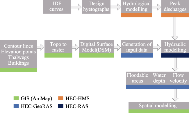
Figure 2 Methodological flowchart describing the stages of this research using different softwares
Pearson linear correlations were determined for the Barcarena and Massamá streams to measure the strength of the association between the longitudinal values of stream bed slope, channel width, flood width (i.e., width of flood extent for an event with a certain return period), water depth and flow velocity. Cross sections every 5 m were drawn perpendicularly to the flow direction to define the longitudinal variations in the channel widths and the flood widths for the events with minimum and maximum RT considered: 2- and 100-year RT, respectively. Longitudinal water depths and flow velocities were also determined every 5 meters (coincident with the width cross sections) and for the lines with the highest values during 2- and 100-year RT events. The correlation coefficients and their significance were obtained using SPSS software.

4 Results

4.1 Floodable areas, water depths and flow velocities

The floodable areas for the 2-, 5-, 10-, 20-, 50- and 100-year RT in the study area can be seen in Figure 1. The estimated peak discharges for the Barcarena (upstream and downstream of the confluence) and the Massamá streams are presented in Table 1. The small size of the Barcarena watershed and the location of the study area in the middle section of the watershed implies that peak discharges are less than 200 m3/s. The shape of the valley bottom and the natural and anthropic features of the stream channels, namely the existence of retaining walls, prevent wide floodable areas (Figure 1 and Table 1). Floodwaters remains confined to the stream channel in some sectors, not overflowing to the floodplain, even during high- magnitude events, which favors a high-energy environment with high flow velocities. The results also point to the interruption of the floodable area on the Massamá stream, where it is culverted under a road, causing the flow accumulation upstream of the hydraulic passage (Figure 1).
Table 1 Peak flows and floodable areas for the n-year RT in the study area
Return
period(RT)
Peak discharges (m3/s) Floodable areas
Barcarena upstream Barcarena downstream Massamá Total
(m2)
Total
(%)
Increase
(m2)
2-year 35.08 41.50 6.22 14,102 51 -
5-year 64.63 74.83 9.37 17,538 63 3436
10-year 85.07 97.62 11.4 19,627 71 2089
20-year 105.45 120.23 13.35 21,817 78 2190
50-year 131.95 149.57 15.84 25,845 93 4028
100-year 152.65 174.59 18.43 27,825 100 1980
Floodable areas for a 2-year RT event represent just over half (51%) of those referring to a 100-year recurrence (Table 1). The floodable area of a 50-year RT event represents 93% of the floodable area for a 100-year RT event. What seems to be a small increase in area (1980 m2) for an event of twice the magnitude (50- to 100-year RT) represents an important increase in the height and volume of floodwaters (m3), expressed by the increment of water depth.
As expected, the highest water depths coincide with the stream channels and, more specifically, with the thalwegs. As the magnitude increases, there are increases in water depths and a consequent progressive occupation of the floodplains (Figure 3). The average water depth increases between 0.98 m (2-year RT) and 1.54 m (100-year RT). Five classes were defined to understand how the water depths are distributed in the floodable areas and how they vary in events with different return periods: ≤ 1 m, 1-2 m, 2-3 m, 3-4 m and > 4 m (Table 2). The percentage of area occupied by the first class (≤ 1 m) ranges between 52% for 2 years and 38% for the 20-year RT. Its importance decreases until the 20-year RT and rises again for the 50- and 100-year RT. This is explained by the overflow of the Barcarena stream in several sections during events with higher return periods. Water depths are naturally lower in the floodplains than in the stream channel, which justifies the growing importance of the lower classes. In the second class (1-2 m), the occupied area decreases with a decrease in frequency, ranging between 42% for the 2-year RT and 25% for the 100-year RT. Between 2 and 3 m, the occupied area increases up to the 10-year RT (22%) and decreases progressively at the highest magnitudes. In the last two classes (3-4 m and > 4 m), the relevance grows with the increase of the return period. However, the higher class is only represented in the 20-, 50- and 100-year RT, while the second higher class is not represented in the estimated results for the 2-year RT (Table 2).
As with the water depth, the highest flow velocities occur along the stream channels (Figure 4), in the sections where the bed slope is more pronounced. The greater roughness justifies the much lower velocities in the floodplains. The flow velocity also tends to be higher downstream and lower upstream of narrower sections, whether they are natural or artificial. This happens close to the hydraulic passage on the Massamá stream (Figures 3 and 4). There is flow accumulation upstream from this infrastructure, widening the floodable areas, while downstream there is a considerable increment in flow velocities. The visible damage in the Massamá stream bed (red circle in Figure 5) demonstrates the high velocities of the floodwaters and the destructive capacity of this tributary until the confluence with the Barcarena stream. On the other hand, flow velocity decreases when the channel becomes wider or there is an overflow of the watercourse into the floodplains. Flow velocity losses also occur upstream of the confluences. Reductions are identified in the Barcarena stream, upstream of the confluence with the Massamá stream, most notable for the higher return periods (Figure 4). This can be explained by the turbulent flow, typical of the convergence between two watercourses during flash floods.
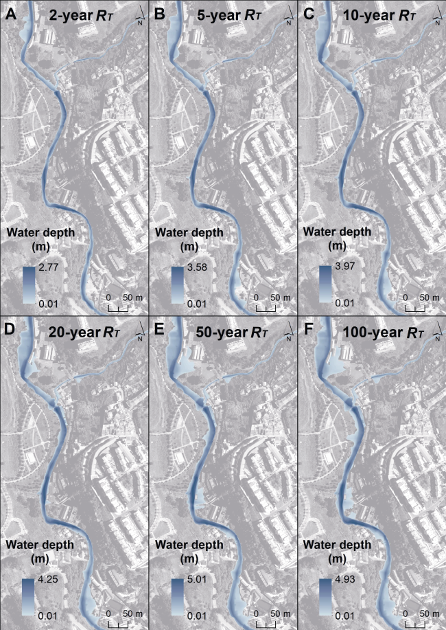
Figure 3 Water depths for the n-year Rr in the study areav
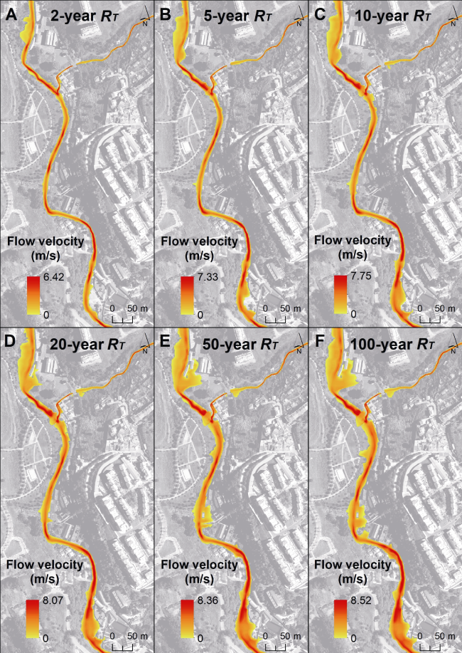
Figure 4 Flow velocities for the n-year RT in the study area
Table 2 Area occupied by each class of water depth in floodable areas for the n-year RT in the study area
Water depth
(m)
Area (%)
2-year RT 5-year RT 10-year RT 20-year RT 50 years RT 100 years RT
≤ 1 52.3 42.4 39.3 37.9 40.5 41.6
1-2 42.2 35.6 32.8 30.5 26.7 24.6
2-3 5.5 20.1 21.8 21.3 19.4 18.7
3-4 0 1.9 6.1 9.8 10.9 12.2
> 4 0 0 0 0.5 2.5 2.9
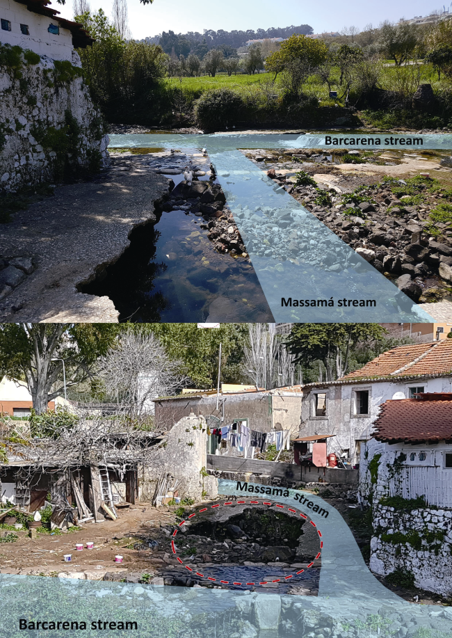
Figure 5 Confluence of the Massamá and Barcarena streams seen from upstream (top) and downstream (bottom). The red circle points to the damage caused by past flood events in the Massamá stream bed
The average flow velocities increase with increasing return periods, ranging between 1.55 m/s for the 2-year and 2.12 m/s for the 100-year RT flood. The five classes (≤ 1 m/s, 1-3 m/s, 3-5 m/s, 5-7 m/s and > 7 m/s) show a more linear pattern when compared to water depths. Thus, higher velocities are more relevant in events of greater magnitude (Table 3). The only exception is the 1-3 m/s class, whose importance grows up to the 10-year RT, reaching more than 50% of the total, and decreases thereafter.
Table 3 Area occupied by each class of flow velocity in floodable areas for the n-year RT in the study area
Flow velocity
(m/s)
Area (%)
2-year RT 5-year RT 10-year RT 20-year RT 50-year RT 100-year RT
≤ 1 38.8 33.5 29.9 28.3 28.9 27.5
1-3 48.1 49.7 50.6 49.9 47.8 46.3
3-5 12.2 14.5 16.0 17.3 18.1 19.7
5-7 0.9 2.2 3.3 4.2 4.8 5.9
> 7 0 0.1 0.2 0.3 0.4 0.6

4.2 Spatial relationships between water depth and flow velocity

Spatial correlations were determined between water depth and flow velocity in the floodable areas for the 2-, 5-, 10-, 20-, 50- and 100-year RT using GIS. Correlation coefficients (R) range between 0.39 for the 5-year RT and 0.50 for the 100-year RT (Table 4). Despite the values are not particularly relevant, which means that the spatial relationships between water depth and flow velocity are not directly proportional, there is an increasing (linear) trend with return periods from 10- to 100-year RT. The increasing discharges lead to the expansion of floodable areas and the progressive occupation of the banks by floodwaters. Both water depths and velocities tend to be low in these areas, unlike what happens along the stream channels, where longitudinal changes in channel geometry/morphology or flow turbulence can affect the flow behavior.
Table 4 Correlation coefficients between water depth and flow velocity in the floodable areas for the n-year RT
Return period (RT) 2-year 5-year 10-year 20-year 50-year 100-year
R 0.40** 0.39** 0.41** 0.43** 0.46** 0.50**

** Correlation is significant at the 0.01 level (2-tailed).

Additionally, two samples of 100 random pixels with a minimum distance of 5 m between them were selected in GIS. The first sample uses water depths and flow velocities of a 2-year RT event and the second uses values of a 100-year RT event (Figure 6). The correlation coefficients are like those presented in Table 4: 0.35 for the 2-year and 0.47 for the 100-year RT (both significant at the 0.01 level).
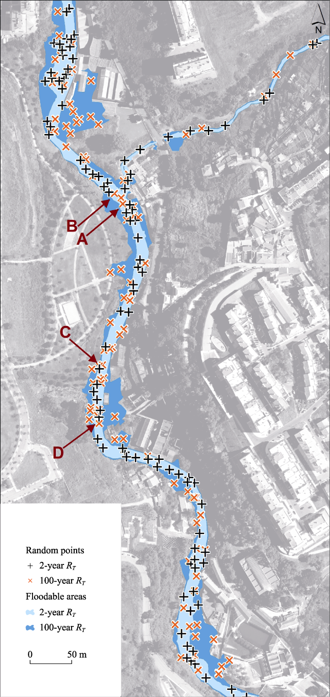
Figure 6 Location of the random points in the floodable areas for the 2- and the 100-year RT Note: A, B, C and D correspond to the four points identified in Figure 9.
By representing the water depth in a curve of increasing values and associating their respective flow velocities, i.e., obtained for the same 100 pixels, two distinct trends in flow velocity in both return periods are identifiable (Figure 7). There is a noticeable increasing trend in flow velocity during the first phase (light orange), following the growing line of water depth. In a second phase (dark orange), the flow velocity tends to decrease as the water depth increases. There is a moment when high water depths are no longer associated with high velocities. There is even a propensity for flow velocity to decrease when the highest water depths are reached. It is confirmed that there is no direct relationship between water depth and velocities. The values of flow velocity can differ by more than 4 m/s for similar water depths in the 2-year RT (Figure 7a) and the 100-year RT (Figure 7b).
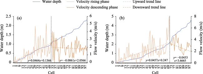
Figure 7 Variation of flow velocity with increasing water depth from the sample of random points for the 2- (a) and the 100-year RT (b)
The opposite exercise represents flow velocities in a curve of increasing values, associating their respective water depths (Figure 8). The results are similar, revealing a first phase (light blue) with an increasing trend of water depth as the flow velocity increases and a second phase (dark blue) with an inverse behavior. When high velocities are achieved it is less likely that water depths will also be high. Still, for similar velocities the results show that water depths can range by more than 2 m in the 2-year RT (Figure 8a) and more than 4 m in the 100-year RT (Figure 8b).
Figure 8 Variation of water depth with increasing flow velocity from the sample of random points for the 2- (a) and the 100-year RT (b)
It is also important to analyze what occurs in the same pixel in all return periods to assess whether the increase in magnitude has consequences on the association between water depth and flow velocity. Of the 100 pixels in the random sample for the highest return period (100-year RT), four represent different types of flow behaviors along the Barcarena stream channel (Figure 9). The location of these four points can be found in Figure 6. The constant increase in water depth and flow velocity with the increase in RT occurs in 60% of the pixels, configuring the most frequent behavior (represented in Figure 9a). The increment in magnitude implies gradual increases in both flow components. However, this type of relationship rarely occurs for very high values. Figure 9b shows the typical flow behavior upstream of confluences and obstacles, in which velocity tends to decrease with increasing water depth. In this case, the highest flow velocity is reached for the 5-year RT, decreasing continuously thereafter, while the water depth is constantly rising. Figure 9c shows an increase in the water depth up to the 50-year RT and an abrupt loss in the 100-year RT, while the flow velocity has a sharp rise. This occurs immediately upstream of an overbank flooding situation, in which the velocities achieved in the previous dozens of meters are substantially higher for the 100-year RT when compared to the lower return periods (visible in Figure 4). The high flow velocity reached consequently leads to a shallower water depth at this point (upstream of the overbank flooding). In the latter type, both components grow progressively, but flow velocity starts to decrease after the 20-year RT as a result of high values of water depth (Figure 9d), causing the overbank flooding (Figure 3). In short, Figure 9a illustrates the most common flow behavior, Figure 9b shows the behavior upstream of a confluence or obstacles, Figure 9c demonstrates the relationship between water depth and velocity immediately upstream of an overbank flooding situation, and Figure 9d represents the flow behavior when overbank flooding occurs.
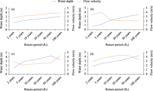
Figure 9 Types of relationships (a, b, c and d) between water depth and flow velocity for the n-year RT from a sample of random points Note: the location of A, B, C and D can be found in Figure 6.

4.3 Maximum values of water depth and flow velocity

The maximum values of water depth range between 2.77 m and 5.01 m (Table 5). The highest maximum value was obtained for the 50-year RT and not for the 100-year RT floods, although the difference is not significant (8 cm). This can be explained by the larger extension of the floodable areas for the 100-year RT and by the way it affects the distribution of water depths. The maximum values of flow velocity reach 6.41 m/s for the 2-year and 8.52 m/s for the 100-year RT (Table 6).
Table 5 Maximum values of water depth for the n-year RT and the flow velocities estimated for the same pixel
Return period (RT) 2-year 5-year 10-year 20-year 50-year 100-year
Water depth (m) 2.77 3.58 3.97 4.25 5.01 4.93
Flow velocity (m/s) 2.36 2.87 3.20 3.55 2.37 2.83
Table 6 Maximum values of flow velocity for the n-year RT and the water depths estimated for the same pixel
Return period (RT) 2-year 5-year 10-year 20-year 50-year 100-year
Flow velocity (m/s) 6.42 7.33 7.75 8.07 8.36 8.52
Water depth (m) 0.52 1.60 1.83 2.03 2.19 2.40
The location of the maximum values of water depth and flow velocity is different and dependent on the magnitude of the flash flood events (Figure 10). On the other hand, increases in the return period can change the location of the maximum water depth and the maximum flow velocity. This can be explained by the progressive flooding of the floodplain with increasing discharges and the consequent greater flood extents, causing changes in the behavior of the flow parameters.
Two locations were identified for the maximum values of water depth: one for the 2- to 20-year RT and another for the 50- and 100-year RT (Figure 10a). These are separated by about 120 meters. Three locations were obtained for the maximum velocities: 1) 2-year RT; 2) 5 to 20-year RT; and 3) 50 and 100-year RT (Figure 10b). Except for the 2-year RT, in which the maximum flow velocity occurs downstream of the hydraulic passage on the Massamá stream (Figure 10b), the maximum values for the remaining recurrences are close to each other in the Barcarena stream. The erosive capacity of both streams in these sectors during flash floods is shown in Figure 10. The maximum values of flow velocity for the 5-, 10- and 20-year RT are located about 10 meters upstream of the maximum values for the 50- and 100-year RT, representing the most critical section regarding flow velocity (Figure 10b). This occurs in a narrow section of the channel and downstream of a bend apex, confirming that the highest velocities in a curved bend can be found further downstream with increasing discharges, as mentioned by Harrison et al. (2015). On the other hand, this critical section is coincident with the lowest roughness segment, where the Barcarena stream is confined between stone walls, and is located downstream of the highest bed slope value in this watercourse: 9.9% (Figure 11).
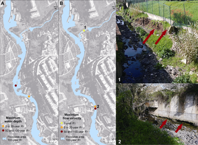
Figure 10 Location of the highest values of water depth (A) and flow velocity (B). Red arrows point to bank erosion where the maximum velocities are achieved in the Massamá (2-year RT) and Barcarena streams (5- to 100-year RT)
The maximum water depth for the 2- to 20-year RT (Figure 10a) is located upstream of the highest flow velocity section (Figure 10b). For the 50- and 100-year RT, this point was found in a section where the floodable area is much wider when compared to what happens upstream and downstream (Figure 10a). Both points are in low bed slope sections: < 2% (Figure 11). In addition to the maximum values not being spatially coincident, the maximum water depths do not correspond to particularly high values of flow velocity and vice versa (Tables 5 and 6). On the other hand, the corresponding flow velocity is higher for events with a 20-year RT (3.55 m/s) than for the 50 (2.37 m/s) or the 100-year RT (2.83 m/s) due to the change in the location of the maximum values of water depth (Figure 10a and Table 5). Even so, all these values are far from the maximum flow velocities estimated for any of the return periods (Table 6), which also occurs for the water depths (Table 5).

4.4 Longitudinal variations in bed slope, roughness, channel width, flood width and flow components

Values of bed slope, roughness, channel width, flood width, water depth and flow velocity along the stream channels were obtained to understand their longitudinal variations in the Barcarena and Massamá streams. The results of the hydraulic modelling showed that, while the highest values of water depth follow the thalwegs, this is not always the case regarding the highest values of flow velocity. So, the lateral position of these lines is not always coincident along the channels.
Correlation coefficients were determined using the longitudinal values of bed slope, channel width, flood width, water depth and flow velocity for the 2- and 100-year RT in the Barcarena and Massamá streams (Table 7). Unlike bed slope and channel width, which do not change with increasing return periods, flood width varies when the magnitude of an event increases. Thus, flood widths can only be associated with water depths and flow velocities with the same return period. Bed slope tends to be negatively correlated to water depth and positively correlated to flow velocity, which means that higher values of slope lead to lower depths and higher velocities. Stronger correlations were found for Massamá stream when compared to the Barcarena stream. Channel width presents a similar behavior to the bed slope (higher widths correspond to lower depths and higher velocities), although with more neglectable values, especially in the Barcarena stream. Flood width has a distinct behavior, with some noteworthy aspects: 1) higher flood widths tend to be more associated with higher depths and lower velocities, which is understandable because wide flood extents are caused by high water depths, resulting in decreases of longitudinal flow velocities; 2) the correlation coefficients are always higher for a 100-year RT event when compared to a 2-year RT event, meaning that the longitudinal variation of water depth and flow velocity are more dependent on the flood width during high-magnitude events; and 3) the correlation coefficient with the longitudinal flow velocity in the Barcarena stream for a 100-year RT event is the highest presented in Table 7 (-0.68).
Table 7 Correlation coefficients between the longitudinal values of bed slope, channel width, flood width, water depth and flow velocity for the 2- and 100-year RT in the Barcarena and Massamá streams
Barcarena Massamá
Water depth Flow velocity Water depth Flow velocity
Return period (RT) 2-year 100-year 2-year 100-year 2-year 100-year 2-year 100-year
Bed slope -0.32** -0.10 0.32** 0.11 -0.57** -0.50** 0.67** 0.65**
Channel width -0.33** -0.11 0.03 -0.13 -0.51** -0.51** 0.33** 0.38**
Flood width 0.18* 0.31** -0.48** -0.68** -0.06 0.46** -0.14 -0.49**

Notes: * Correlation is significant at the 0.05 level (2-tailed); ** Correlation is significant at the 0.01 level (2-tailed)

The influence of bed slope in the longitudinal variations (along the thalwegs) of water depths and flow velocities can be confirmed in Figure 11. Higher depths are spatially related to low values of slope, while the maximum velocities are coincident with high slope and low roughness sections. Nevertheless, other factors like channel width, flood width/overbank flooding or the presence of obstacles can affect longitudinal water depths and flow velocities. Despite the relationship between depth and velocity is not particularly strong when considering the floodable areas (Table 4), this becomes more relevant along the streamlines. There are strong negative relationships between longitudinal water depths and flow velocities, with the two flow components moving in opposite directions. The correlation coefficients (R) for the Barcarena stream reach -0.78 and -0.66 for the 2- and 100-year RT events, respectively. More relevant values are achieved for the Massamá stream (-0.83 and -0.87) for the same RT events because this is a smaller watercourse with limited overbank flooding, leading to a more direct relationship between the two flow components. The smaller flood width/extent also explains the higher correlation coefficients during a 2-year RT event when compared to a 100-year RT event along the Barcarena stream. If floodwaters are confined between the walls of the stream channel, there are fewer factors that interfere with their longitudinal flow behavior.
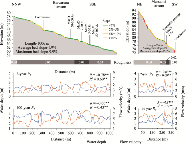
Figure 11 Longitudinal variations of bed slope, roughness, water depth, and flow velocity in the Barcarena and Massamá streams Notes: MaxD-maximum water depth; MaxV-maximum flow velocity; RT-return period; ** Correlation is significant at the 0.01 level (2-tailed).

5 Discussion

Complex interactions between water depths and flow velocities occur during flash flood events. Flow velocity is probably the most sensitive flow parameter, with longitudinal, lateral and vertical variations in response to changes in channel geometry and morphology (width, depth and sinuosity), differences in bed slope, modifications in channel and floodplains roughness, the presence of confluences and obstacles (bridges, hydraulic passages or weirs), or the extension of floodable areas and variations in flood stage. Thus, velocity is also the hardest flow component to model, especially for flash flood situations.
1D models assume that water flows in one dominant direction aligned with the centerline of the stream channel (Balica et al., 2013), computing velocities between cross-sections and not predicting the 2D nature of the flow (USACE, 2009). This is highly significant in sharp bends and areas of confluence between watercourses, where secondary flows are relevant
(Shao et al., 2003; Ottevanger et al., 2012; Khan et al., 2013; Liu et al., 2014; Gholami et al., 2015; Biscarini et al., 2016). The results of hydraulic modelling for the study area indicate that the highest velocities occur in the center of the stream channels, which is true for narrow channels (as in the study area) and for straight sections (Mudd, 2006; Pradhan et al., 2018; Mirauda and Russo, 2019). On the other hand, the lateral redistribution of flow velocity is negligible in mildly curved bends but highly relevant in sharp bends (Ottevanger et al., 2012). In these sections, the maximum flow velocity core moves from the inner (convex) channel wall at the beginning of the curve towards the outer (concave) wall at the end of the curve (Patra et al., 2004; Gholami et al., 2015; Harrison et al., 2015). Therefore, the downstream part of the outer wall is especially affected by erosion (Ottevanger et al., 2012; Biscarini et al., 2016). It can then be said that the 1D hydraulic model used in this research can represent the flow velocities correctly in straight sections or in mildly curved bends, which are present in most of the study area. On the other hand, there are certainly errors in the curved sections and at the confluence between the Barcarena and the Massamá streams, something that could be minimized by 2D models (Patra et al., 2004; Cook and Merwade, 2009; Balica et al., 2013; Crispino et al., 2015; Gibson and Pasternack, 2016) or could even be overcome by 3D models (Shao et al., 2003; Ottevanger et al., 2012).
The fact that the higher velocities are located on the center area of the channel leads to the misrepresentation of the lateral distribution of velocities in sharper curves. This also prevents the spatial relationship between water depths and flow velocities in the floodable areas from being more significant, although high correlation coefficients were not expectable because there are numerous factors that influence this relationship (e.g., geometry, slope, or roughness). Similar results were found by Kreibich et al. (2009). On the other hand, a more significant relationship was achieved considering the longitudinal lines with highest values of water depth and flow velocity. Strong negative correlation coefficients between the two flow components were found in the study area. Water depth and flow velocity seem to influence each other decisively, with increases in water depth associated with decreases in velocity and vice versa. The results of Stephenson and Kolovopoulos (1990), Tarekul et al. (2009) and Xing et al. (2016) evidence the same flow behavior. The correlation coefficients are even more significant in the Massamá stream because floodwaters are more frequently confined between the channel walls when compared to the Barcarena stream, invalidating the effect of overbank flooding, and increasing the influence of bed slope or channel width on the longitudinal flow behavior.
The results shown in Figures 7 and 8 revealed that flow velocities tend to grow with increasing water depths and vice versa. However, this trend is reversed when high values of water depth or flow velocities are achieved, which only happen along the stream channels. This inversion of the flow behavior can be explained by previously mentioned factors, namely changes in channel geometry, morphology or slope, and by the presence of confluences and obstacles. The highest water depths occur in sections with low bed slope or upstream of an obstacle, where flow velocities significantly drop. On the contrary, the highest flow velocities occur in sections with high slopes or downstream of an obstacle. In these sections water depths decrease because high velocities do not allow the accumulation of floodwaters. These spatial relationships between stream channel features and flow components justify the two phases shown in Figures 7 and 8, as well as the location of the maximum values of water depth and flow velocity.
Unlike what happens with water depth, the obtained results suggest that higher longitudinal velocities may happen for lower return period events in the same pixel. This translates the flow complexity during flash flood events, with several factors interfering in the longitudinal flow behavior. The joint action of bed slope, roughness, channel morphology and geometry, flood width, the presence of obstacles, and the mutual influence of water depth and flow velocity explains the longitudinal variations in both flow components.
The choice of the steady-state regime in this study is a topic that should be discussed. In theory, the unsteady-state condition can be considered more suitable for flash flood modelling purposes, allowing to better account for the changes in flow regime and dynamics, mainly in floodplains. However, this study aims to model designed floods associated with different return periods-and particularly the depth-velocity relation during the flood peak -, rather than a particular or past flood event, and to measure the spatial relationships between flow components and channel features in space. For this reason, the development of the flood hydrograph along the time was not considered in this study. On the other hand, Barcarena is a small watershed, with narrow stream channels and floodplains in the study area, situations in which the option for a steady-state condition is suitable (SEPA, 2017; Hocini et al., 2021).
The use of a 2D model may improve the obtained results, ensuring that the lateral distribution of flow velocities would be represented more correctly by the hydraulic model. Nevertheless, several studies have demonstrated that there are no significant differences in the results between 1D and 2D models, except in curved sections, and that the quality of these results are strongly related to the accuracy of available data (Horritt and Bates, 2002; Jowett and Duncan, 2012; Gharbi et al., 2016; Maharjan and Shakya, 2016). Jowett and Duncan (2012) even state that the correlations between predicted and measured water depths and flow velocities were higher for 1D when compared to 2D models. Additionally, HEC-RAS and HEC-GeoRAS (1D) provide good results representing the longitudinal variations in flow velocity.
The lack of hydrometric data compromises the calibration and validation of the flow velocity results, something that was also highlighted in other studies (e.g., Moramarco et al., 2011, Asano and Uchida, 2016, Chen et al., 2020). The elevation data used to build the DSM is the other main source of uncertainty in this study. The non-existence of LiDAR elevation data compromises the quality of the DSM in the floodplains and the same happens with the lack of elevation data along the stream channels. However, by including the position of the thalwegs in the ArcMap’s Topo to Raster tool, the transversal and longitudinal variations in the elevation along the stream channels are guaranteed. This allows a more accurate representation of the hydrological behavior during flood events. This can be a useful and easy solution to improve the quality of the DSM and, consequently, the hydrologic modelling results in areas with scarce or no elevation data along the river/stream channels.
Quite often, flood boundaries and depths suffice in informing spatial planning instruments regarding the definition of zoning regulations for land use. However, at higher scales of intervention-particularly regarding urban environments and hydraulic infrastructures, like bridges and other crossings -, it becomes mandatory to consider the relationship of water depth and flow velocity as characteristics of flood hazard. Several matrices exist that combine water depths and flow velocities and define thresholds for human, vehicle and building’s stability (e.g., Smith and Cox, 2019), also considered on the flood risk maps produced under the European Floods Directive.
A comprehensive understanding of the depth-velocity relationship is necessary to adequately select the most suitable solution at each location. When the impacts on the built environment alone are considered, a detailed characterization of that relationship allows to select and implement the most adequate building codes and safety standards and to inform the insurance risk analysis.
As in regard to the safety of buildings and infrastructure, the relationship between water depth and flow velocity is critical in defining thresholds for human instability during a flood (Cox et al., 2010). This is a field in which urban design, architecture and civil protection intersect focusing on the safety of pedestrians, both resident and transient, studying the location of solutions such as handrails, grips and raised elements (part of sidewalks and heavy benches not movable by floodwaters), for example. In fact, flow dynamics is distinct depending on the width of streets, type of crossing, existence of open spaces and their spatial relationship with streets (Bernardini et al., 2017). Based on the depth-velocity relationship, the objective is to help identify evacuation routes and safety areas, even if located within a vaster floodable area, with stagnant floodwaters or without flooding.
In resume, a detailed characterization of the flood behavior under urban and morphologic conditions, when coupled with simulations of the pedestrians, vehicles and buildings’ response, can provide valuable knowledge to act preventively by combining diverse domains of planning-urban, spatial, environmental and civil protection-and reduce flood impacts.
Despite the uncertainties, the results obtained in this study show evident associations between water depths and flow velocities and with some of their influencing factors (bed slope, channel width or flood width). This research also demonstrates the potentialities and the added value provided by spatial analysis in GIS.

6 Conclusions

The short period between the triggering rainfall and the peak discharge, as well as the high flow velocities, solid loads and erosive capacity make flash floods particularly dangerous when compared to other types of flooding. The combination between water depth and flow velocity defines the energy head, flow force, carrying capacity, destructive power and, ultimately, the flash flood hazard, being fundamental to the stability and safety of people and vehicles in floodwaters and to the damage caused in buildings and infrastructures.
The HEC-RAS/HEC-GeoRAS software provides good results in the definition of floodable areas and water depths, however it has limitations in determining the flow velocities, especially in their lateral distribution under complex flow conditions. Still, the longitudinal distribution of flow velocity along the stream channels revealed a good performance in reproducing the flow behavior during flash flood events.
The highest velocities occur in sections with high bed slopes, low roughness coefficients, along narrow channels/sections and where floodwaters are confined to the channel walls, with significant flow velocity decreases when the flood stage exceeds the overbank level. High values of flow velocity are also achieved downstream of natural or anthropic obstacles located in the stream channels. The highest water depths are found in sections with low bed slopes and upstream of narrow sections or obstacles. Therefore, the location of the maximum values of water depth and flow velocity are not spatially coincident. Maximum water depths are not associated with very high velocities and maximum velocities are not associated with higher water depths. Contrasting trends in the relationships between water depths and flow velocities were identified along the centerlines, demonstrating that when the values of one of the flow components increase, the other tends to behave in the opposite way. The longitudinal values of water depths and flow velocities are strongly and negatively associated, with higher correlation coefficients for the Massamá stream. The correlation coefficients between bed slope, channel width, water depths and flow velocities are also higher in the Massamá stream when compared to the Barcarena stream.
In addition to the geometric, morphological, slope and roughness characteristics of the stream channels, also the magnitude of a flash flood event has a significant influence on the behavior of water depth and flow velocity. The values of both flow components tend to increase with increasing return periods. Nevertheless, and depending on the location in the flooded area, the increment in discharges can result in an overbank flooding which alters their most common behavior. This means that, as the flood stage increases, the estimated flow velocity for a 5-year RT event can be higher than for a 100-year RT event on the same pixel located in the stream channel. On the other hand, the increasing magnitude can change the location of the maximum values of both flow components.
This research proves the usefulness of GIS regarding spatial analysis, which can improve the knowledge on the relationships between water depths and flow velocities during flash flood events. The cartography of the hydraulic modeling results, the identification of critical sections, the location of the maximum values of water depth and flow velocity or the development of spatial correlations are advantages of GIS in flood research. This information and knowledge can be useful for spatial planning, hydraulic structures’ design and emergency management. Understanding and quantifying the relationships between water depth and flow velocity in flooded areas is fundamental for risk assessment and management, although better elevation data for channels and floodplains and flow data during flash flood events are necessary to improve the results.

Acknowledgements

The authors would like to thank the Oeiras City Hall for providing the elevation data. This work was funded by the Research Unit (UIDB/00295/2020 and UIDP/00295/2020). Miguel Leal and Pedro Pinto Santos were funded by the FCT-Portuguese Foundation for Science and Technology, I.P. through the grant SFRH/BD/96632/2013 and the contract CEEIND/ 00268/2017, respectively. Eusébio Reis was financed by national funds through FCT, under the framework of the project BeSafeSlide-Landslide Early Warning soft technology prototype to improve community resilience and adaptation to environmental change (PTDC/ GES-AMB/30052/2017).

Data Availability Statement

The data that support the findings of this study are available upon request to the authors. The primary data belong to the Oeiras City Hall and, therefore, cannot be made publicly available.
[1]
Abt S R, Wittier R J, Taylor A et al., 1989. Human stability in a high flood hazard zone. Journal of the American Water Resources Association, 25(4): 881-890. https://doi.org/10.1111/j.1752-1688.1989.tb05404.x.

[2]
Aronica G T, Candela A, Fabio P et al., 2012. Estimation of flood inundation probabilities using global hazard indexes based on hydrodynamic variables. Physics and Chemistry of the Earth, 42-44: 119-129. https://doi.org/10.1016/j.pce.2011.04.001.

[3]
Arrighi C, Oumeraci H, Castelli F, 2017. Hydrodynamics of pedestrians’ instability in floodwaters. Hydrology and Earth System Sciences, 21(1): 515-531. https://doi.org/10.5194/hess-21-515-2017.

[4]
Asano Y, Uchida T, 2016. Detailed documentation of dynamic changes in flow depth and surface velocity during a large flood in a steep mountain stream. Journal of Hydrology, 541(Part A): 127-135. https://doi.org/10.1016/j.jhydrol.2016.04.033.

[5]
Balica S F, Popescu I, Beevers L et al., 2013. Parametric and physically based modelling techniques for flood risk and vulnerability assessment: A comparison. Environmental Modelling & Software, 41: 84-92. https://doi.org/10.1016/j.envsoft.2012.11.002.

[6]
Bernardini G, Postacchini M, Quagliarini E et al., 2017. A preliminary combined simulation tool for the risk assessment of pedestrians’ flood-induced evacuation. Environmental Modelling & Software, 96: 14-29. https://doi.org/10.1016/j.envsoft.2017.06.007.

[7]
Biscarini C, Di Francesco S, Ridolfi E et al., 2016. On the simulation of floods in a narrow bending valley: The Malpasset dam break case study. Water, 8(11): 545. https://doi.org/10.3390/w8110545.

[8]
Blanckaert K,de Vriend H J, 2010. Meander dynamics: A nonlinear model without curvature restrictions for flow in open-channel bends. Journal of Geophysical Research Earth Surface, 115(F4): F04011. https://doi.org/10.1029/2009JF001301.

[9]
Brandão C, Rodrigues R, Costa J P, 2001. Análise de fenómenos extremos: Precipitações intensas em Portugal Continental. Direcção dos Serviços de Recursos Hídricos, Lisbon.

[10]
Chen X, Chen L, Stone M C et al., 2020. Assessing connectivity between the river channel and floodplains during high flows using hydrodynamic modeling and particle tracking analysis. Journal of Hydrology, 583: 124609. https://doi.org/10.1016/j.jhydrol.2020.124609.

[11]
Chimene C A, Campos J N B, 2020. The design flood under two approaches: Synthetic storm hyetograph and observed storm hyetograph. Journal of Applied Water Engineering and Research, 8(3): 171-182. https://doi.org/10.1080/23249676.2020.1787242.

[12]
Chow V T, Maidment D R, Mays L W, 1988. Applied Hydrology. New York: Mc-Graw-Hill.

[13]
Cook A, Merwade V, 2009. Effect of topographic data, geometric configuration and modeling approach on flood inundation mapping. Journal of Hydrology, 377: 131-142. https://doi.org/10.1016/j.jhydrol.2009.08.015.

[14]
Cox R J, Shand T D, Blacka M J, 2010. Appropriate safety criteria for people. WRL Research Report 240. Report for Institution of Engineers Australia, Australian Rainfall and Runoff Guidelines: Project 10.

[15]
Crispino G, Gisonni C, Iervolino M, 2015. Flood hazard assessment: Comparison of 1D and 2D hydraulic models. International Journal of River Basin Management, 13(2): 153-166. https://doi.org/10.1080/15715124.2014.928304.

[16]
de Moel H, Jongman B, Kreibich H et al., 2015. Flood risk assessments at different spatial scales. Mitigation and Adaptation Strategies for Global Change, 20: 865-890. https://doi.org/10.1007/s11027-015-9654-z.

[17]
Diakakis M, Deligiannakis G, Pallikarakis A et al., 2016. Factors controlling the spatial distribution of flash flooding in the complex environment of a metropolitan urban area. The case of Athens 2013 flash flood event. International Journal of Disaster Risk Reduction, 18: 171-180. https://doi.org/10.1016/j.ijdrr.2016.06.010.

[18]
Elkhrachy I, 2015. Flash flood hazard mapping using satellite images and GIS tools: A case study of Najran City, Kingdom of Saudi Arabia (KSA). The Egyptian Journal of Remote Sensing and Space Science, 18(2): 261-278. https://doi.org/10.1016/j.ejrs.2015.06.007.

[19]
Fontana N, Marini G,De Paola F, 2013. Experimental assessment of a 2-D entropy-based model for velocity distribution in open channel flow. Entropy, 15(3): 988-998. https://doi.org/10.3390/e15030988.

[20]
Geravand F, Hosseini S M, Ataie-Ashtiani B, 2020. Influence of river cross-section data resolution on flood inundation modeling: Case study of Kashkan river basin in western Iran. Journal of Hydrology, 584: 124743. https://doi.org/10.1016/j.jhydrol.2020.124743.

[21]
Gharbi M, Soualmia A, Dartus D et al., 2016. Comparison of 1D and 2D hydraulic models for floods simulation on the Medjerda River in Tunisia. Journal of Materials and Environmental Science, 7(8): 3017-3026.

[22]
Gholami A, Bonakdari H, Zaji A H et al., 2015. Simulation of open channel bend characteristics using computational fluid dynamics and artificial neural networks. Engineering Applications of Computational Fluid Mechanics, 9(1): 355-369. https://doi.org/10.1080/19942060.2015.1033808.

[23]
Gibson S A, Pasternack G B, 2016. Selecting between one-dimensional and two-dimensional hydrodynamic models for ecohydraulic analysis. River Research and Applications, 32(6): 1365-1381. https://doi.org/ 10.1002/rra.2972.

[24]
Grimaldi S, Petroselli A, Serinaldi F, 2012. Design hydrograph estimation in small and ungauged watersheds: Continuous simulation method versus event-based approach. Hydrological Processes, 26(20): 3124-3134. https://doi.org/10.1002/hyp.8384.

[25]
Habib M, Alzubi Y, Malkawi A et al., 2020. Impact of interpolation techniques on the accuracy of large-scale digital elevation model. Open Geosciences, 12(1): 190-202. https://doi.org/10.1515/geo-2020-0012.

[26]
Hammond M J, Chen A S, Djordjević S et al., 2015. Urban flood impact assessment: A state-of-the-art review. Urban Water Journal, 12(1): 14-29. https://doi.org/10.1080/1573062X.2013.857421.

[27]
Harrison L R, Dunne T, Fisher G B, 2015. Hydraulic and geomorphic processes in an overbank flood along a meandering, gravel-bed river: Implications for chute formation. Earth Surface Processes and Landforms, 40(9): 1239-1253. https://doi.org/10.1002/esp.3717.

[28]
Hocini N, Payrastre O, Bourgin F et al., 2021. Performance of automated methods for flash flood inundation mapping: A comparison of a digital terrain model (DTM) filling and two hydrodynamic methods. Hydrology and Earth System Sciences, 25(6): 2979-2995. https://doi.org/10.5194/hess-25-2979-2021.

[29]
Horritt M S, Bates P D, 2002. Evaluation of 1D and 2D numerical models for predicting river flood inundation. Journal of Hydrology, 268(1-4): 87-99. https://doi.org/10.1016/S0022-1694(02)00121-X.

[30]
Hutchinson M F, Gallant J C, 2000. Digital elevation models and representation of terrain shape. In: Wilson J P, Gallant J C(eds.), Terrain Analysis:Principles and Applications. New York: John Wiley & Sons, 29-50.

[31]
Jonkman S N, Penning-Rowsell E, 2008. Human instability in flood flows. Journal of the American Water Resources Association, 44(5): 1208-1218. https://doi.org/10.1111/j.1752-1688.2008.00217.x.

[32]
Jonkman S N, Vrijling J K, 2008. Loss of life due to floods. Journal of Flood Risk Management, 1(1): 43-56. https://doi.org/10.1111/j.1753-318x.2008.00006.x.

[33]
Jowett I G, Duncan M J, 2012. Effectiveness of 1D and 2D hydraulic models for instream habitat analysis in a braided river. Ecological Engineering, 48: 92-100. https://doi.org/10.1016/j.ecoleng.2011.06.036.

[34]
Karvonen R A, Hepojoki A, Huhta H K et al., 2000. The use of physical models in dam-break analysis. RESCDAM final report, Helsinki: Helsinki University of Technology.

[35]
Keifer C J, Chu H H, 1957. Synthetic storm pattern for drainage design. Journal of the Hydraulics Division, 83(4): 1-25. https://doi.org/10.1061/JYCEAJ.0000104.

[36]
Khan M S M, Al Amin M A, Rahman M M et al., 2013. An experimental study of longitudinal velocity distribution at cross-over and bend section of a compound meandering channel. American Journal of Civil Engineering, 1(3): 124-128. https://doi.org/10.11648/j.ajce.20130103.16.

[37]
Khatami S, Khazaei B, 2014. Benefits of GIS application in hydrological modeling: A brief summary. VATTEN-Journal of Water Management and Research, 70(1): 41-49.

[38]
Kreibich H, Piroth K, Seifert I et al., 2009. Is flow velocity a significant parameter in flood damage modelling? Natural Hazards and Earth System Sciences, 9(5): 1679-1692. https://doi.org/10.5194/nhess-9-1679-2009.

[39]
Kvočka D, Falconer R A, Bray M, 2016. Flood hazard assessment for extreme flood events. Natural Hazards, 84: 1569-1599. https://doi.org/10.1007/s11069-016-2501-z.

[40]
Lastra J, Fernández E, Díez-Herrero A et al., 2008. Flood hazard delineation combining geomorphological and hydrological methods: An example in the Northern Iberian Peninsula. Natural Hazards, 45: 277-293. https://doi.org/10.1007/s11069-007-9164-8.

[41]
Leal M, Ramos C, Pereira S, 2018. Different types of flooding lead to different human and material damages: The case of the Lisbon Metropolitan Area. Natural Hazards, 91: 735-758. https://doi.org/10.1007/s11069-017- 3153-3.

[42]
Leal M, 2019. Inundações na Área Metropolitana de Lisboa: Danos humanos e materiais e componentes do risco[D]. PhD thesis in Geography, Institute of Geography and Spatial Planning, Universidade de Lisboa.

[43]
Leal M, Boavida-Portugal I, Fragoso M et al., 2019. How much does an extreme rainfall event cost? Material damage and relationships between insurance, rainfall, land cover and urban flooding. Hydrological Sciences Journal, 64(6): 673-689. https://doi.org/10.1080/02626667.2019.1595625.

[44]
Liu C, Wright N, Liu X et al., 2014. An analytical model for lateral depth-averaged velocity distributions along a meander in curved compound channels. Advances in Water Resources, 74: 26-43. https://doi.org/10.1016/j. advwatres.2014.08.003.

[45]
Maharjan L B, Shakya N M, 2016. Comparative study of one dimensional and two dimensional steady surface flow analysis. Journal of Advanced College of Engineering and Management, 2: 15-30. https://doi.org/10. 3126/jacem.v2i0.16095.

[46]
Marini G, De Martino G, Fontana N et al., 2011. Entropy approach for 2D velocity distribution in open-channel flow. Journal of Hydraulic Research, 49(6): 784-790. https://doi.org/10.1080/00221686.2011.635889.

[47]
Merz B, Thieken A H, Gocht M, 2007. Flood risk mapping at the local scale:Concepts and challenges. In: BegumS, StiveM J F, HallJ W ( vol.eds.), Flood Risk Management in Europe. Advances in Natural and Technological Hazards Research. Dordrecht: Springer, 25, pp. 231-251. https://doi.org/10.1007/978-1-4020-4200-3_13.

[48]
Merz B, Kreibich H, Schwarze R et al., 2010. Review article “assessment of economic flood damage”. Natural Hazards and Earth System Sciences, 10(8): 1697-1724. https://doi.org/10.5194/nhess-10-1697-2010.

[49]
Meyer V, Scheuer S, Haase D, 2009. A multicriteria approach for flood risk mapping exemplified at the Mulde River, Germany. Natural Hazards, 48: 17-39. https://doi.org/10.1007/s11069-008-9244-4.

[50]
Middelmann-Fernandes M H, 2010. Flood damage estimation beyond stage-damage functions: An Australian example. Journal of Flood Risk Management, 3(1): 88-96. https://doi.org/10.1111/j.1753-318X.2009.01058.x.

[51]
Mirauda D, Russo M G, 2019. Information entropy theory applied to the dip-phenomenon analysis in open channel flows. Entropy, 21(6): 554. https://doi.org/10.3390/e21060554.

[52]
Mohanty L, Patra K C, Khatua K K et al., 2014. Modelling the depth-averaged velocity in trapezoidal meandering channels. ISH Journal of Hydraulic Engineering, 20(1): 111-118. https://doi.org/10.1080/09715010.2013. 857472.

[53]
Moramarco T, Saltalippi C, Singh V P, 2011. Velocity profiles assessment in natural channels during high floods. Hydrology Research, 42(2/3): 162-170. https://doi.org/10.2166/nh.2011.064.

[54]
Mudd S M, 2006. Investigation of the hydrodynamics of flash floods in ephemeral channels: Scaling analysis and simulation using a shock-capturing flow model incorporating the effects of transmission losses. Journal of Hydrology, 324(1-4): 65-79. https://doi.org/10.1016/j.jhydrol.2005.09.012.

[55]
Na W, Yoo C, 2018. Evaluation of rainfall temporal distribution models with annual maximum rainfall events in Seoul, Korea. Water, 10(10): 1468. https://doi.org/10.3390/w10101468.

[56]
Ottevanger W, Blanckaert K, Uijttewaal W S J, 2012. Processes governing the flow redistribution in sharp river bends. Geomorphology, 163/164: 45-55. https://doi.org/10.1016/j.geomorph.2011.04.049.

[57]
Pappenberger F, Matgen P, Beven K J et al., 2006. Influence of uncertain boundary conditions and model structure on flood inundation predictions. Advances in Water Resources, 29(10): 1430-1449. https://doi. org/10.1016/j.advwatres.2005.11.012.

[58]
Patra K C, Kar S K, Bhattacharya A K, 2004. Flow and velocity distribution in meandering compound channels. Journal of Hydraulic Engineering, 130(5): 398-411. https://doi.org/10.1061/(ASCE)0733-9429(2004)130:5 (398).

[59]
Penning-Rowsell E, Johnson C, Tunstall S et al., 2005. The Benefits of Flood and Coastal Risk Management:A Handbook of Assessment Techniques. Middlesex University Press. https://doi.org/10.1596/978-0-8213- 8050-5.

[60]
Pradhan A, Kumar Khatua K, Sankalp S, 2018. Variation of velocity distribution in rough meandering channels. Advances in Civil Engineering, 1-12. https://doi.org/10.1155/2018/1569271.

[61]
Ramos C, Reis E, 2001. As cheias no Sul de Portugal em diferentes tipos de bacias hidrográficas. Finisterra, 36(71): 61-82. https://doi.org/10.18055/Finis1648.

[62]
Ramos C, Reis E, 2002. Floods in southern Portugal: Their physical and human causes. Mitigation and Adaptation Strategies for Global Change, 7(3): 267-284. https://doi.org/https://doi.org/10.1023/A:1024475529524.

[63]
Santos P P, Reis E, 2017. Assessment of stream flood susceptibility: A cross-analysis between model results and flood losses. Journal of Flood Risk Management, 11(Suppl.2): 1038-1050. https://doi.org/10.1111/jfr3.12290.

[64]
SEPA, 2017. Flood Modelling Guidance for Responsible Authorities, version 1.1. Edinburgh: Scottish Environment Protection Agency.

[65]
Shao X, Wang H, Chen Z, 2003. Numerical modeling of turbulent flow in curved channels of compound cross-section. Advances in Water Resources, 26(5): 525-539. https://doi.org/10.1016/S0309-1708(03)00008-3.

[66]
Smith G, Cox R, 2019. Safety design criteria. In: Ball J, Babister M, Nathan R et al. (eds.), Australian Rainfall and Runoff: A Guide to Flood Estimation, Book 6-Flood Hydraulics, Commonwealth of Australia, pp. 246-274.

[67]
Smith K, 1991. Environmental Hazards: Assessing Risk and Reducing Disaster. London: Routledge.

[68]
Soetanto R, Proverbs D G, 2004. Impact of flood characteristics on damage caused to UK domestic properties: The perceptions of building surveyors. Structural Survey, 22(2): 95-104. https://doi.org/10.1108/02630800410538622.

[69]
Song S, Schmalz B, Zhang J X, et al., 2017. Application of modified Manning formula in the determination of vertical profile velocity in natural rivers. Hydrology Research, 48(1): 133-146. https://doi.org/10.2166/ nh.2016.131.

[70]
Sordo-Ward Á, Bianucci P, Garrote L et al., 2014. How safe is hydrologic infrastructure design? Analysis of factors affecting extreme flood estimation. Journal of Hydrologic Engineering, 19(12): 04014028. https://doi.org/10.1061/(ASCE)HE.1943-5584.0000981.

[71]
Stephenson D, Kolovopoulos P, 1990. Effects of momentum transfer in compound channels. Journal of Hydraulic Engineering, 116(12): 1512-1522. https://doi.org/10.1061/(ASCE)0733-9429(1990)116:12(1512).

[72]
Tarekul I G M, Yoshihisa K, Nobuyuki T, 2009. Flood flow analysis during rising and falling stages in a doubly meandering compound channel. In: ZhangC, TangH (eds.), Advances in Water Resources and Hydraulic Engineering. Berlin Heidelberg: Springer, 387-392. https://doi.org/10.1007/978-3-540-89465-0_68.

[73]
Thieken A H, Müller M, Kreibich H et al., 2005. Flood damage and influencing factors: New insights from the August 2002 flood in Germany. Water Resources Research, 41(12): 1-16. https://doi.org/10.1029/2005WR004177.

[74]
Ţîncu R, Zêzere J L, Lazar G, 2018. Identification of elements exposed to flood hazard in a section of Trotus River, Romania. Geomatics, Natural Hazards and Risk, 9(1): 950-969. https://doi.org/10.1080/19475705.2018.1486891.

[75]
Trigo R M, Ramos C, Pereira S S et al., 2016. The deadliest storm of the 20th century striking Portugal: Flood impacts and atmospheric circulation. Journal of Hydrology, 541(Part A): 597-610. https://doi.org/10.1016/j.jhydrol.2015.10.036.

[76]
USACE, 2009. HEC-GeoRAS: GIS Tools for Support of HEC-RAS using ArcGIS. User’s Manual. U.S. Army Corps of Engineers.

[77]
Werner M G F, 2004. A comparison of flood extent modelling approaches through constraining uncertainties on gauge data. Hydrology and Earth System Sciences, 8(6): 1141-1152. https://doi.org/10.5194/hess-8-1141-2004.

[78]
Xia J, Teo F Y, Lin B et al., 2011. Formula of incipient velocity for flooded vehicles. Natural Hazards, 58: 1-14. https://doi.org/10.1007/s11069-010-9639-x.

[79]
Xia J, Falconer R A, Wang Y et al., 2014. New criterion for the stability of a human body in floodwaters. Journal of Hydraulic Research, 52(1): 93-104. https://doi.org/10.1080/00221686.2013.875073.

[80]
Xing Y, Yang S, Zhou H et al., 2016. Effect of floodplain roughness on velocity distribution in mountain rivers. Procedia Engineering, 154: 467-475. https://doi.org/10.1016/j.proeng.2016.07.539.

[81]
Zhang H, Li Z. Saifullah M et al., 2016. Impact of DEM resolution and spatial scale: Analysis of influence factors and parameters on physically based distributed model. Advances in Meteorology, 8582041. https://doi.org/10.1155/2016/8582041.

[82]
Zhang Q, Shi Y, Xiong M, 2009. Geometric properties of river cross sections and associated hydrodynamic implications in Wuhan-Jiujiang river reach, the Yangtze River. Journal of Geographical Sciences, 19: 58-66. https://doi.org/10.1007/s11442-009-0058-4.

[83]
Zimmermann M, Pozzi A, Stoessel F, 2005. VADEMECUM. Hazard maps and related instruments. The Swiss system and its application abroad. Capitalisation of experience. PLANAT, the Swiss National Platform Natural Hazards. Bern: Swiss Agency for Development and Cooperation.

Outlines

/