Research Articles

Incorporation of intra-city human mobility into urban growth simulation: A case study in Beijing

  • WANG Siying , 1, 2 ,
  • FEI Teng 1 ,
  • LI Weifeng 2, 3 ,
  • ZHANG Anqi 2 ,
  • GUO Huagui 5 ,
  • DU Yunyan , 4, *
Expand
  • 1. School of Resource and Environmental Science, Wuhan University, Wuhan 430079, China
  • 2. Department of Urban Planning and Design, The University of Hong Kong, Hong Kong, China
  • 3. Guangdong-Hong Kong-Macau Joint Laboratory for Smart Cities
  • 4. Institute of Geographic Sciences and Natural Resources Research, CAS, Beijing 100101, China
  • 5. School of Architecture and Urban-rural Planning, Fuzhou University, Fuzhou 350108, China
* Du Yunyan, Professor, E-mail:

Wang Siying, PhD Candidate, specialized in urban analytics. E-mail:

Received date: 2021-05-12

  Accepted date: 2021-12-17

  Online published: 2022-07-25

Supported by

Wuhan University “351” Talent Plan Teaching Position Project

Guangdong-Hong Kong-Macau Joint Laboratory Program of the 2020 Guangdong New Innovative Strategic Research Fund from Guangdong Science and Technology Department(2020B1212030009)

Abstract

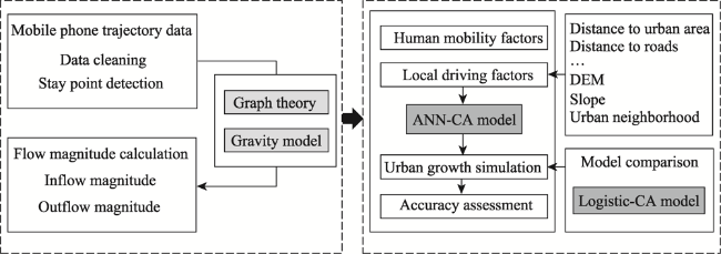
The effective modeling of urban growth is crucial for urban planning and analyzing the causes of land-use dynamics. As urbanization has slowed down in most megacities, improved urban growth modeling with minor changes has become a crucial open issue for these cities. Most existing models are based on stationary factors and spatial proximity, which are unlikely to depict spatial connectivity between regions. This research attempts to leverage the power of real-world human mobility and consider intra-city spatial interaction as an imperative driver in the context of urban growth simulation. Specifically, the gravity model, which considers both the scale and distance effects of geographical locations within cities, is employed to characterize the connection between land areas using individual trajectory data from a macro perspective. It then becomes possible to integrate human mobility factors into a neural-network-based cellular automata (ANN-CA) for urban growth modeling in Beijing from 2013 to 2016. The results indicate that the proposed model outperforms traditional models in terms of the overall accuracy with a 0.60% improvement in Cohen’s Kappa coefficient and a 0.41% improvement in the figure of merit. In addition, the improvements are even more significant in districts with strong relationships with the central area of Beijing. For example, we find that the Kappa coefficients in three districts (Chaoyang, Daxing, and Shunyi) are considerably higher by more than 2.00%, suggesting the possible existence of a positive link between intense human interaction and urban growth. This paper provides valuable insights into how fine-grained human mobility data can be integrated into urban growth simulation, helping us to better understand the human-land relationship.

Cite this article

WANG Siying , FEI Teng , LI Weifeng , ZHANG Anqi , GUO Huagui , DU Yunyan . Incorporation of intra-city human mobility into urban growth simulation: A case study in Beijing[J]. Journal of Geographical Sciences, 2022 , 32(5) : 892 -912 . DOI: 10.1007/s11442-022-1977-6

1 Introduction

As one of the most complex systems, cities constantly evolve (White et al., 2015). The intrinsic nature of urban changes lies in the myriad of human activities that significantly impact land-use patterns. The rapid growth of population and the increasing need for socio-economic development has led to considerable land-use and land-cover changes, including the expansion of urban areas, biodiversity changes, and changes in ecosystem services (Liu et al., 2014; Zhao et al., 2020). The study of urban growth modeling can help us to better understand the driving factors, dynamics, and consequences of future land use (Marta and Luis, 2021). It can thus provide practical urban planning and management suggestions (Li and Yeh, 2002).
The cellular automata (CA) models have gained popularity among various land-use models as they have introduced dynamic features in the spatial simulation of urban growth (Berling-Wolff and Jianguo, 2004). After Tobler (1979) first adopted CA in geographic modeling, various urban growth simulations applied similar models over the last few decades (Couclelis, 1985, 1997; Santé et al., 2010; Liu et al., 2014; Liang et al., 2018). Many studies have successfully demonstrated that CA model simulations are a practical approach in representing complex spatial processes (Batty et al., 1997). By properly defining transition rules, global spatio-temporal patterns can emerge from local interactions among adjacent land units (Santé et al., 2010; Liu et al., 2017). Many published studies have demonstrated the potential of CA-based models. For example, the SLEUTH model, using two coupled cellular automata for urban growth and land-use change simulations, have been applied for many years (Clarke, 2008); more recently, the FLUS model, which combines top-down system dynamics and natural effects in land-use simulations, has shown its power and superiority compare with other models (Liu et al., 2017).
Aside from the ongoing, promising advances in the empirical techniques adopted in CA models, it is also vital to better understand the driving factors that affect the existing spatial distribution of different land-use types. In CA models, urban growth simulation involves various spatial variables inputs (Lin and Li, 2015) and the neighborhood’s exogenous conditions. In general, the factors can be aggregated into two categories (White and Engelen, 1993): 1) fixed conditions, e.g., road, water, and 2) suitability factors, e.g., slope, soil type. However, these driving factors generally remain stationary and any changes that do occur, proceed at a much slower rate than the fast urbanization processes. Therefore, one current focus is to integrate new sources of information that can further characterize the interchange between different places, for example, urban information flow and population flow.
Human mobility is suspected of exerting long-term impacts on urban developmental processes (Lee and Holme, 2015; Chen et al., 2019). The relationships between human mobility and land-use types are complex and often bi-directional. The accumulation of individual human trajectories between areas significantly influences long-term land-use patterns. Furthermore, different land-use functions serve a diverse suite of urban activities. This interchange of different flows can form an urban network and thus represent the relationships between different places. Several studies have successfully attempted to integrate mobility data into urban growth simulations, and it has proven advantageous. In the study by Li (2018) and Lin (2015), web search data from Baidu were extracted to present the spatial flows within urban agglomerations. These simulation results suggested that an urban flow variable enhances the performance of CA models. Most recently, Xia et al. (2019) proposed an improved CA model, in which weighted urban flows were obtained by information and population flow data represented by a gravitational field model. The result indicated that the spatial interaction data could improve the urban growth simulation accuracy in large-scale metropolitan areas.
However, most current research only coarsely quantifies the mobility effects. The referenced urban networks generally formed among different cities but failed to depict the relationship within the city. Specifically, most of the mobility data adopted are population flow data and web search data at the city level, sufficient for describing the inter-city spatial relationship in an urban agglomeration but difficult to extend into a finer geographical space (intra-city level). Moreover, information flow from web searching data cannot represent the pressure that human flow brings to land use in the real world. Therefore, fresh insight needs to be explored by combining high-resolution intra-city mobility data into urban growth simulation, such as trajectory data.
Given the current widespread use of smartphones and the full coverage of connection networks in big cities, cell-phone signaling record data has become popular in urban mobility studies (Zhang, 2014; Liu et al., 2018; Wang et al., 2018). A well-known study demonstrated that individual daily mobility is highly predictable and shows a highly reproducible pattern (González et al., 2008). Therefore, it should be safe to assume that the travel patterns of all residents in a city on a given random complete weekday are representative of their travel patterns over time. In this paper, an artificial-neural-network-based CA (ANN-CA) model considering the human mobility pattern is proposed for an urban growth simulation. Concerning the high urbanization rate in megacities like Beijing, we want to explore how the human flow within a city can help to promote our understanding of urban growth. The proposed model is distinct in coupling the spatial interactions from massive cell-phone signaling record datasets in the simulation input process. More importantly, such intra-city trajectory data are of high spatial resolution and can reasonably describe the real-world human movements within an entire city. By quantifying the urban flow magnitudes based on graph theory and a gravity model, this study can provide a refreshing view of the relationship between urban land teleconnections and urban growth.
This paper is organized into five sections. In Section 2, we introduce the relevant materials and methods, describing critical theories of the proposed methods and placing human mobility into the context of land use simulation. Section 3 presents the application of the methodology, the comparison of the simulation results with various models, and sensitivity analyses. Sections 4 and 5 discuss the results and present the conclusions.

2 Methodology

The proposed methodology is composed of two parts: (1) designing an approach to processing the massive trajectory data and quantifying the intra-city inflow and outflow magnitudes, and (2) coupling the spatial interactions according to the driving factors that the ANN-CA model uses to simulate urban growth. The general framework of the approach is illustrated in Figure 1.
Figure 1 The framework of the ANN-CA model in the integration of human mobility factors

2.1 Measurement of flow magnitude in the city

2.1.1 Stay point detection

It is crucial to partition the data into meaningful elements when dealing with massive trajectory data, which is important for further analysis. Considering the different semantics of human mobility, the recorded locations of trajectories are not all equally important. Therefore, stay points, where individuals tend to conduct meaningful activities like working, shopping, etc., need to be extracted.
Operationally, a stay point is constrained by both spatial and temporal dimensions. If people remain within a certain region within a given time interval, the location is detected as a stay point. The process is shown in Figure 2. The individual’s trajectory, P, is represented by a sequence of points {p1, p2, p3, …, pn}. Each point contains three properties (latitude, longitude, and timestamp). The points are sequentially connected based on their chronological order. Then, a subsequence of P, {pm, pm+1, pm+2, …, pm+j}, can be regarded as one set of stay points, if:
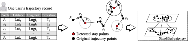
Figure 2 Illustration of the stay point detection process
1) Distance (pm, pi) ≤ Dth, m < i m+j
2) Time interval (pm, pm+j) ≥ Tth
where Dth is the distance threshold and Tth is the time threshold.
The complexity of the processed data can be effectively reduced compared to the original trajectory data. At the same time, the semantic meanings behind the trajectories can be enhanced. All the calculations forthcoming is based on these processed trajectories.

2.1.2 Graph-based flow magnitude calculation

Location-to-location movements within a city can reflect the spatial mobility pattern of people. These movements, also referred to as spatial interactions (or flows), naturally form large geographically embedded networks (Guo, 2009). Literature regarding land changes has discussed distal flows can be regarded as urban land teleconnections that drive and respond to urbanization (Seto et al., 2012). The gravity model is the most common formula for quantifying spatial interactions (Yan and Zhou, 2018; Hilton et al., 2020). Specifically, it allows us to measure location-based relationships by integrating the distance decay functions with measures of the relative scale of geographical entities (Haynes and Fotheringham, 1985). The model has become a popular method for quantifying the urban spatial interaction intensity (or magnitudes) between cities by leveraging different kinds of urban flow data (Lin and Li, 2015; Li et al., 2018; Xia et al., 2019; Lu et al., 2021).
Although both approaches are based on gravity models, this method differs from previous studies. Existing studies (Lin and Li, 2015; Li et al., 2018; Xia et al., 2019; Lu et al., 2021) were mainly conducted in urban agglomeration areas. The scale of urban flow data (e.g., human migration, information flow) is region-wide, and the data only depicts city-to-city spatial interactions. Such native coarse scales of the spatial interaction data make it challenging to consider the heterogeneity in each cell’s interaction strength in a gravity model. However, the principle of gravity model operates under the premise that in addition to the distance, the attraction between two places is also dependent on the products of the masses (e.g., population, GDP) of these two places. In our research, benefitting from fine data granularity, we can leverage the complex graph theory and form a massive trajectory network among mobile phone stations. Thus, the degree centrality of each station can be considered in the gravity model to describe the origin and destination attractiveness. In this way, we can obtain weighted spatial flow magnitudes for many base stations within the city and then derive reasonable grid representations for each cell using a spatial interpolation technique.
The processed trajectories record people moving between different places, and those stay points on the same trajectory are thus correlated. For each trajectory, the nature of the connection is assumed to exist between any two stay points in chronological order. For example, if a person’s daily trajectory is recorded as S = {s1, s2, s3, s4}, then the links will be {s1s2, s2s3, s3s4, s1s3, s1s4, s2s4}. Following graph theory, we constructed a weighted graph (also called a network) G = (V, E) using those links of the trajectory data (Figure 3), where V represents the set of nodes (locations, in this research, refers to mobile phone base stations), and E is the set of edges (spatial interactions, also called flows). To measure the weight (wij) of the edges of the trajectory network, the concept of connection strength is proposed as we operate under the assumption that each spatial location in the city varies in its attraction for people.
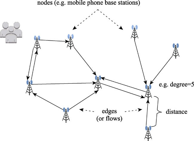
Figure 3 An example of a directed graph formed by human trajectories
In graph theory, the more people that visit a location, the higher the degree centrality of this node. In the gravity model, the connection between two nodes is inversely proportional to their distance, usually represented by distance decay functions. In general, there are three distance decay functions: the power law, exponential law, and Gaussian function (Yu et al., 2014). Previous research has most often adopted the exponential function in characterizing urban mobility patterns (Liang et al., 2011); therefore, we choose this approach for our method. It follows that, based on the relationship between degree and distance, the connection strength, wij, between mobile phone stations i and j is given as
${{w}_{ij}}=\frac{minmax({{k}_{i}}*{{k}_{j}})}{{{e}^{-\alpha d}}}~~(\alpha >0)$
where ki and kj are the degrees of node i and node j, respectively, minmax is the function by which the products of degrees are normalized, d is the distance between mobile phone base stations i and j, and α is the distance decay coefficient.
To distinguish between the direction of spatial interaction, we classify urban flows as either inflow or outflow. Based on the accumulation function, the sum of inflow and outflow magnitudes for each mobile phone station is calculated by:
$F^{in}=\sum_{i}^{m} w_{i j} * a_{ij}^{in}$..,
$F^{out}=\sum_{i}^{n} w_{i j} * a_{ij}^{out}$.,
where m and n are the number of nodes in-connected and out-connected with nodes i, wij is the connection strength of the edge between node i and node j, and aij and aji are the in-degree and out-degree values of node i, which can be derived from the adjacency matrix of the trajectory network.
Subsequently, the weighted inflow and outflow magnitudes of a massive number of stay points are obtained from the original complex trajectory data. Given the high density and relatively uniform distribution of sites, this study used the spatial interpolation technique to interpolate the inflow and outflow magnitudes of detected station points into 30 m raster layers. This process was implemented in the ArcGIS environment. Both inverse distance weighted (IDW) interpolation and kriging tools have been considered for interpolation. We used the trial-and-error method to test each scenario. By manually adjusting parameters and comparing the smoothness of the resulting surfaces, the ordinary kriging method with the optimized parameters offered by ArcGIS was chosen to generate the raster layers of flow magnitude. In this way, we can quantify the impact of human mobility interaction in each cell.

2.2 The framework of the ANN-CA model

The ANN-CA model is selected to perform the urban growth modeling task (Figure 4). Cellular automata (CA) is a discrete, intrinsically spatial model that ties nicely into geographic information systems (GIS). The relaxation of its transition rules enhances the capabilities of a CA model to deal with the actual evolution of land-use patterns. To reconcile the complex relationship between spatial variables, an artificial neural network method is adopted to calculate the overall development probability of each cell.
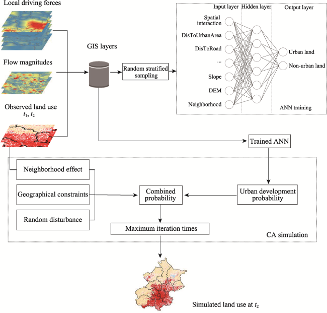
Figure 4 The architecture of the ANN-CA model
Artificial neural networks (ANNs) refer to a family of machine learning algorithms. Using a backward-propagating learning algorithm, ANNs can efficiently learn the multivariate non-linear relationship between different inputs through the learning and training processes (Li and Yeh, 2002). The basic structure of an ANN can be seen in Figure 4. In the input layer, the neurons correspond to the driving factors which ultimately determine the land use development probability. Then, the input variables feed-forward into the next layer with variable weights, and the activation function delivers the outputs. The mathematical expression is given by
$P_{j}^{l}=f\left( \sum\nolimits_{i=1}^{{{n}_{l-1}}}{w_{ji}^{l}\text{*}P_{i}^{l-1}+w_{j0}^{l-1}} \right)$,
where $P_{j}^{l}$ is the output value of node j in the current layer and $P_{i}^{l-1}$ is the input value of the i-th node in the previous layer, nl–1 is the total number of nodes in the previous layer,
$w_{ji}^{l}$ denotes the weight between two layers, and the standard sigmoid function has been chosen as the activation function f (x)=1/(1+ex). In the output layer, the nodes correspond to urban land and non-urban land. For an input land cell n, the development probability is expressed as Pn.
Meanwhile, the transformation of a land cell to urban land is also dependent on other conditions, including the neighborhood effect, geographical constraints, and random disturbances, all of which are accounted for by the CA simulation procedure. Finally, the combined probability of a cell converting into urban land at time t can be given by
$CP_{n}^{t}=P_{n}^{t}\times \text{ }\!\!\Omega\!\!\text{ }_{n}^{t}\times con\times (1+{{[-\text{ln}(\gamma )]}^{\alpha }})$,
where $P_{n}^{t}$ is an estimated development probability that cell n transitions to land use type m at time t. The symbol $~\text{ }\!\!\Omega\!\!\text{ }_{n}^{t}~$denotes the density of urban land in a 5 × 5 Moore neighborhood; con refers to the geographical constraints, such as the ecological control areas, basic farmland protection areas – the value will be assigned as 0 in these areas –; 1+[–ln(γ)]α is the stochastic disturbance term, where γ is a random variable within the range of 0 to 1, and α is an adjustable parameter that controls the size of the stochastic disturbance.
Hence, the iterative procedure of estimating the combined probability for each land cell will begin for the urban growth simulation (Figure 4). At each iteration time, all the exogenous factors are obtained to compute the combined probability for each cell. The current non-urban cell will then be allocated to the urban land if the combined probability exceeds a pre-defined threshold (0.8), set according to previous studies (Guan et al., 2005, Zhou et al., 2017). Then the state of the neighborhood and cell will be updated at each iteration. The process is carried out iteratively until the total number of pixels changed meets the demand for overall urban growth.
To demonstrate the robustness of the effect of spatial interaction within a CA urban growth simulation, a well-accepted traditional logistic-CA model (Lin et al., 2011) was implemented for comparison. Therefore, four models were established, including ANN-CAwithflow, ANN-CAwithoutflow, Logistic-CAwithflow, and Logistic-CAwithoutflow, where withflow indicates a model considering the urban flow effect and withoutflow neglects the urban flow effect.

2.3 Model performance evaluation

Two assessments are used to evaluate model performance: 1) the fit of the ANN model to the development probability and 2) the pixel-based accuracy evaluations of the simulation results.
For the first aspect, the Receiver Operating Characteristic (ROC) curve analysis is adopted to quantify whether the ANN model fits well with the generated overall development performance. The ROC is a common metric to evaluate the classifier system (Lin et al., 2011). Generally, the area under the ROC curve (AUC) was calculated to assess the performance of a model. The value of AUC is generally between 0.5-1; the larger the value of AUC, the better the model’s performance.
For the second aspect, the two most adopted methods used to evaluate the simulation accuracy are Cohen’s Kappa coefficient and the figure of merit (FoM). The Kappa coefficient is designed to measure inter-raster reliability and has been widely used in remote sensing classification measurements (Kerr et al., 2015). By analogy, researchers also apply it to measure the proportion of agreement between the observed raster and simulated raster (Liu et al., 2017; Xia et al., 2019). The Kappa coefficient can be calculated by
$kappa=\frac{p_{0}-p_{e}}{1-p_{e}}=\frac{\frac{1}{N} \sum_{i=1}^{c} n_{i i}-\frac{1}{N^{2}} \sum_{i=1}^{c} n_{i T} * n_{T i}}{1-\frac{1}{N^{2}} \sum_{i=1}^{c} n_{i T} * n_{T i}}$.,
where p0 indicates the agreement between observed raster and simulated raster and pe is the expected probability of chance agreement; N is the total number of cells, c is the number of land-use types; nii is the number of cells in the same category between the two rasters; niT and nTi represent the total number of cells in each category i of the two rasters, respectively.
The FoM can evaluate model accuracy by measuring the agreement of variations between actual land-use patterns and simulation results while ignoring those cells that persist unchanged. The index can be calculated as follows:
$FOM=\frac{B}{(A+B+C)}$.,
where A is the number of errors for those observed urban cells predicted as the persistence of non-urban cells, B is the number of correct cells observed and correctly simulated as urban growth, and C is the number of errors due to observed unchanged cells predicted as urban cells.

3 Implementation and results

3.1 Study area and data preparation

The proposed method was applied in Beijing, the capital of China (Figure 5). The city is located in North China and lies between 39°26′N-41°03′N and 115°25′E-117°30′E. As a megacity, Beijing has a population of over 21.7 million within an area of 16,800 km2. Beijing is now experiencing a high level and low speed of urbanization, distinct from other Chinese cities experiencing dramatic changes in land use. In this case, it is worth examining how human mobility has brought vitality and changes to urban growth in this city. Meanwhile, Beijing has a high mobile phone penetration rate among Chinese cities. Hence, the availability of mobile phone data makes Beijing an ideal research area.
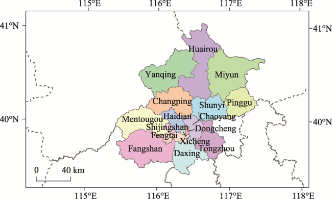
Figure 5 Administration divisions of Beijing
This research centers upon an urban growth simulation from 2013 to 2016, classified from Landsat 8 Operational Land Imager (OLI) images. The spatial resolution is maintained at its initial value of 30 m. Based on existing literature (Gharbia et al., 2016, Qiang and Lam, 2015), the selected driving factors can be classified into four categories (Table 1), including 1) physical properties, 2) proximity to entities of interest (EOI), 3) neighborhood, and 4) human mobility. The physical properties include elevation and slope. Among the proximity properties, the distance to primary roads, secondary roads, and water areas are important indicators for urban growth (Figure 6). As existing urban areas greatly affect newly developed urban areas (Batty, 2005), the distance to urban areas is also considered in this model. Rather than directly calculating the distance from urban centers or gathering discrete urban land-use units, we adopt a more precise way by using night-time light remote sensing data to extract/define urban areas in Beijing supplemented by threshold-based algorithms in the research of Jing et al. (2015). Moreover, the cellular neighborhood always indicates spatial autocorrelation among land cells. A calculation of the number of neighborhood cells is also served as inputs.
Table 1 Model inputs and their data source
Spatial variables Category Explanation Data source
y Binary Urban growth 2013-2016 Landsat 8 Operational Land Imager images
DisToMainRoad Float Euclidean distance to main roads Road network map
DisToSecondRoad Float Euclidean distance to secondary roads Road network map
DisToWaterArea Float Euclidean distance to a water area Map of water area
DisToUrbanArea Float Euclidean distance to an urban area VIIRS Day/Night Band (DNB) Nighttime Imagery
DEM Float Transition suitability considering terrain conditions data Global Digital Elevation Model (ASTGTM)
Slope Float
Neighborhood Float Amount of urban cells in 5·5 neighborhood Landsat 8 Operational Land Imager images
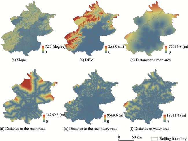
Figure 6 The spatial variables in Beijing (a) slope, (b) DEM, (c) distance to urban area, (d) distance to the main road, (e) distance to the secondary road, and (f) distance to water area
The nature of human mobility in Beijing is inferred by a dataset of mobile phone records used to measure people’s spatial interactions. The dataset is collected from a Chinese mobile communication service provider, who anonymously processed the records to protect personal information. It contains the trajectories of 12,270,000 users and 346,302,792 records on a weekday (27 December 2016) and covers 20,978 mobile phone base stations. Every time a user’s phone connects to the cellular network, a record is generated with a location of the base station and a timestamp. Thus, a sequence of locations represents the trajectory of one user in a day. Figure 7 shows the flow map of the original trajectory data.
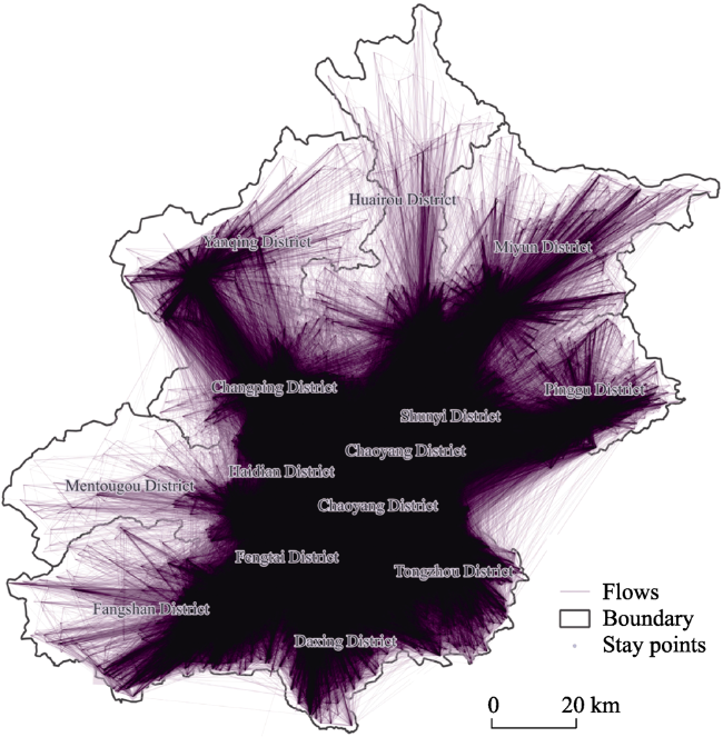
Figure 7 The flow map of trajectory data in Beijing

3.2 Processing of spatial variables and model setup

3.2.1 Stay points detection

The trajectory data was processed according to the methodology section 2.1. Previous studies have described the details of the thresholds setting of stay points detection (Li et al., 2008, Zheng et al., 2009). The commonly used time threshold is 30 min. The distance threshold was usually set to less than 1000 meters, commonly 200 and 500 meters. Based on the average nearest distance (261 meters) among base stations in our research, the distance threshold is set to 500 meters, and the time threshold is set to 30 minutes. After the stay points extraction process, the number of valid trajectories was reduced to 6,650,348, and the total records decreased to 10,033,174 compared to the original data.

3.2.2 Flow magnitude maps

After extracting the abovementioned stay points, we need to quantify the flow magnitude between them. At first, with the formed undirected network (graph) among whole points, a 20,978 × 20,978 adjacency matrix was derived, which stores the adjacent information (edge) between each two mobile phone station points. Then, according to equation (1), the connection strength (edge weight) is calculated between each pair of points based on their in-out degree and distance. On this basis, the inflow magnitude and outflow magnitude of each mobile phone station point can finally be acquired based on equations (2) and (3), respectively. Considering that the distribution of station points is not homogeneous, to match the CA model’s spatial scale, the ordinary kriging method mentioned in section 2.1.2 was used to interpolate the flow magnitude of whole station points onto a 30 m grid surface. Accuracy was assessed by the root mean square error (RMSE) with values of 10.154 and 9.903 for the inflow and outflow magnitude interpolation results, respectively. Figure 8 shows the final flow magnitude layers. As can be observed, the hotspots of inflow magnitude are generally the same as outflow magnitude. At the same time, the distribution pattern outflow tends to be more diffuse. This phenomenon is intuitive in that intended destinations of people are more concentrated in certain functional urban areas, e.g., business, shopping, healthcare, transit.
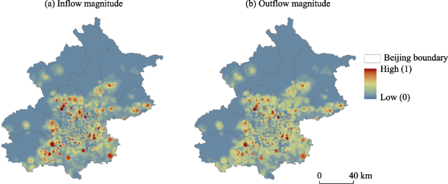
Figure 8 The inflow magnitude distribution (a) and the outflow magnitude distribution (b) of Beijing

3.2.3 Predictive modeling

We project the relevant, collected, and processed variables in the same spatial resolution. All data is normalized in the range of [0, 1] to accelerate the gradient descent algorithm in the ANN model. The overall urban growth pattern is unbalanced, with most of the land cells remaining unchanged while a relatively small number of cells change from non-urban land to urban land. The learning process may have a low sensitivity to the minority class and be affected by the majority class in such a way that it always predicts the land use as unchanged, which is a common problem in the machine learning algorithm called “class imbalance” (Batista et al., 2004; Qazi and Raza, 2012). Thus, an under-sampling technique was adopted to remove samples from the majority class to alleviate this imbalance in the dataset (Bunkhumpornpat et al., 2011; Lemaître et al., 2017). Then the sampled data were randomly stratified and split into two parts, the training dataset (70%) and the testing dataset (30%). The above sampling strategies can optimize the training process and guarantee good model convergence. In this way, a neural network was established for the estimation of overall development probability, and the CA evolution of urban growth was subsequently simulated.

3.3 Simulation results

The four models (ANN-CAwithflow, ANN-CAwithoutflow, Logistic-CAwithflow, and Logistic-CAwithoutflow) proposed in this study are established for the urban growth simulation in Beijing of China from 2013 to 2016 at a spatial resolution of 30 m × 30 m. The simulation results of the four models are shown in Figure 9. Four regions are enlarged to display additional details to better examine the spatial variability among the different simulation results. Compared to the actual land use in 2016, the two ANN-CA models can yield more reliable results than the Logistic-CA models in some fast-growing regions, such as the fourth enlarged area (Daxing District). Specifically, the results of the ANN-based model can generate a more reasonable amount and distribution of urban land. However, due to the large scope of the entire city, it is difficult to visually evaluate the effect of human mobility on the simulation results. Therefore, the evaluation can be made more objective by quantitative assessment.
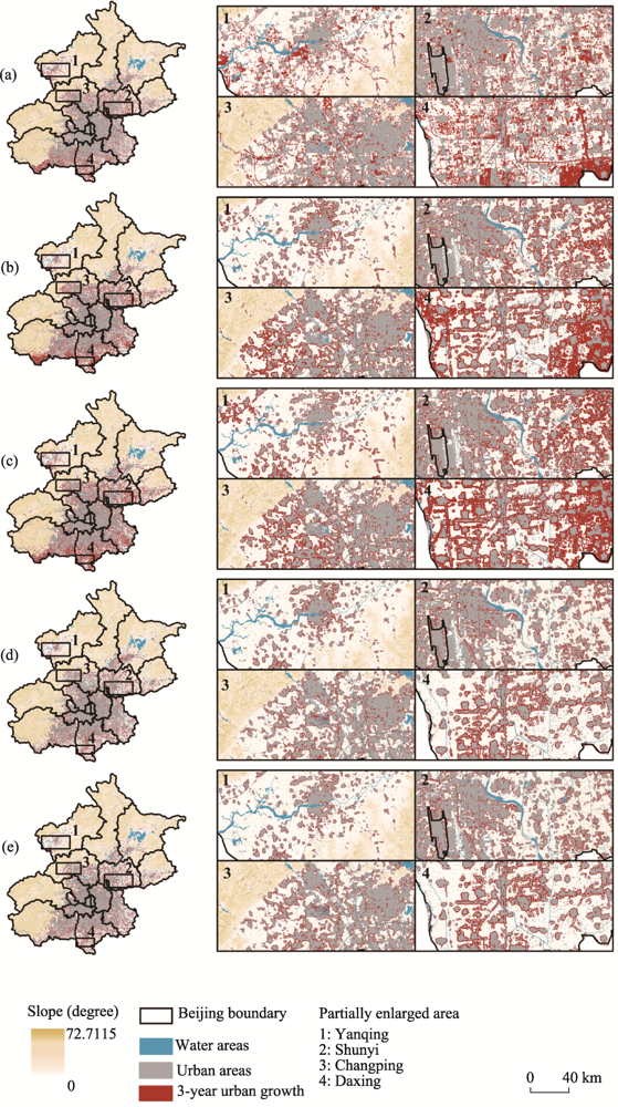
Figure 9 The observed urban growth from 2013 to 2016 in Beijing (a) and the simulated pattern in 2016 based on the four proposed models: (b) ANN-CAwithflow, (c) ANN-CAwithoutflow, (d) Logistic-CAwithflow, and (e) Logistic-CAwithoutflow
The model goodness of fit was examined by the three measures proposed in section 2.3, including ROC, Kappa coefficients, and FoM. Table 2 shows the model accuracy results. The three metrics assessed the degree of model optimization by comparing the results between the models with and without flow. In general, the ANN-CA models outperformed the Logistic-CA models regardless of whether the human mobility factor was considered. The main reason for this could be that the ANN models are more capable of dealing with complex spatial relationships among variables. Moreover, the accuracies of the CA models considering human mobility factors (with flow) are better than that of traditional models (without flow), although the improvements brought about by human flow are generally less significant compared to those attributed to different modeling methods. Regardless, we document improvements of 0.60% for both AUC and the Kappa coefficient and 0.41% for the FoM values relative to the ANN-CAwithflow model.
Table 2 Assessment of the simulation results
Models AUC Improvement Kappa Improvement FoM Improvement
ANN-CAwithflow 0.909 0.60% 0.751 0.60% 0.2362 0.41%
ANN-CAwithoutflow 0.903 - 0.745 - 0.2321 -
Logistic-CAwithflow 0.897 0.40% 0.737 0.30% 0.2115 0.33%
Logistic-CAwithoutflow 0.893 - 0.734 - 0.2082 -
As the newly developed urban cells only accounted for a small portion of the whole city and were concentrated in certain areas, evaluating the model accuracy in different districtswould be more meaningful. Kappa coefficients and FoM values were selected for district-level simulation accuracy assessments. Based on the ANN-CAwithflow model, the improvements of Kappa coefficients and FoM values were calculated for all 16 districts in Beijing (Figure 10) and compared to the traditional model (ANN-CAwithoutflow). It can be seen that most districts maintained significant improvements, except for very few regions that experienced reduced Kappa coefficients and FoM values. Compared with the improvements calculated for the entire city of Beijing, these results on a district basis are more informative. Specifically, by considering the human mobility factors in the ANN-CA model, the improvement of Kappa coefficients in six districts exceeds 0.5%, and in three districts exceeds 2.0%. For FoM, six districts had more than a 0.5% improvement, three districts exceeded 1.0%, and one district exceeded a 2% improvement. We note that several districts, including Chaoyang, Daxing, and Shunyi, are firmly at the forefront of improved Kappa coefficients and FoM values, confirming a satisfactory performance of the ANN-CA model considering human flow.
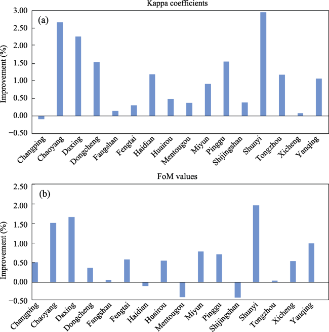
Figure 10 Resultant improvements of Kappa coefficients and FoM values of the simulation results for districts of Beijing based on ANN-CAwithflow model

4 Discussion

A massive spatio-temporal trajectory dataset can serve as a reasonable proxy for human mobility (Chen et al., 2019). The spatial interactions between different land cells can effectively indicate urban growth. Figure 11 shows the accuracy and model loss of the two ANN-CA modeling processes. As can be seen from Figures 11a and b, after 160 epochs, the accuracy values of the model considering flow data stabilize around 0.705, and its losses stabilized between 0.690 and 0.700. In comparison, the accuracy values of ANN-CAwithoutflow stabilize under 0.705, and the losses are around 0.710, respectively. These results support the premise that the inclusion of the spatial interaction patterns of human trajectories does help to improve the ANN modeling performance.
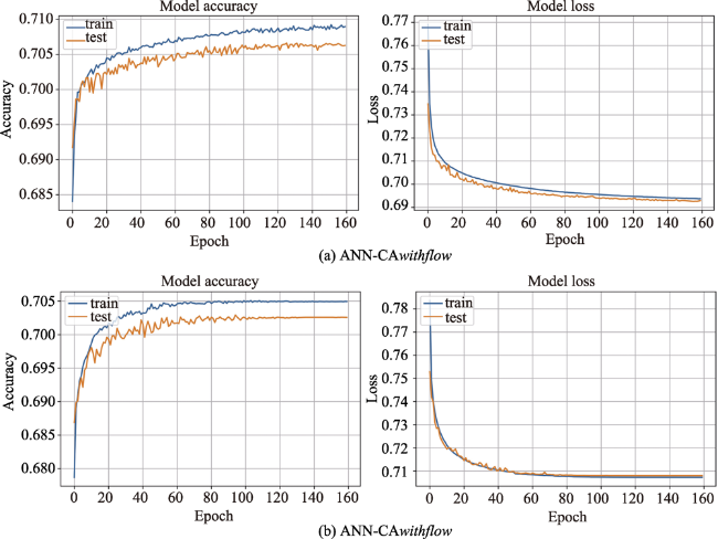
Figure 11 The plots of training accuracy and loss
Although the overall improvements of the simulation results were not prominent (0.41% and 0.60%), the results are reasonable if we compare them with similar research. Xia et al. (2019) conducted urban growth simulations by applying inter-city population flow data and web search engine data and noted improvements between 0.40%-0.59%.
Moreover, we should consider the urbanization of Beijing from a contemporary perspective. In the three years between 2013 and 2016, like most megacities, Beijing’s urbanization level has stabilized, and the speed of urbanization has lessened. Unlike the formerly observed rapid outward urban sprawl, the recent urban growth is different, geared more towards densifying inner-urban areas (Ouyang, 2020). In this context, the dispersive and small changes in the urban area will make the prediction even more difficult for each model, which could be the main reason for the minor numerical improvements attributed to enhancing the model by adding human mobility factors.
However, significant improvements in simulation accuracy do occur in certain districts. The comparisons between different districts may help illustrate the effectiveness of incorporating human mobility into the ANN-CA model and the spatial pattern of this difference. Figure 12 shows the aggregated flow map between 16 districts in Beijing. The spatial interaction within Beijing forms an urban mobility network, with red color and broad lines indicating stronger connections. This map shows strong linkages at the city center, and the flow magnitude is higher between those districts surrounding the core districts (Dongcheng and Xicheng). After comparing the calculated improvements for each district, we found the more significant improvements are partial to Daxing, Chaoyang, and Shunyi districts. All three districts surround the core area of Beijing and keep a close connection with other districts and maintain a higher flow magnitude. More importantly, unlike Changping district, which is located near the higher-elevation region (mountainous area), these three districts are located on the southeast side of the city at a lower elevation, which provides favorable geographical conditions for urban growth. Table 3 compares the elevation of the four mentioned districts. The elevation factor may help us understand why these districts have a more pronounced improvement in simulation results. Those non-urban areas with a strong connection with core urban regions are also more likely to develop because frequent spatial interactions serve as a potential indicator for space consumption and economic development. Therefore, human mobility may constitute a significant connection channel between micro and macro urban development.
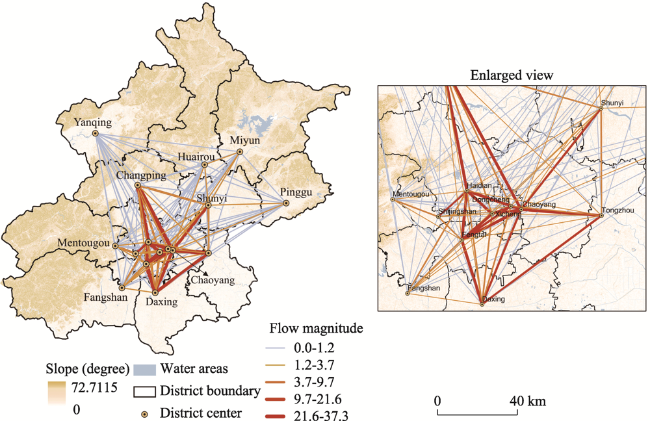
Figure 12 Flow map and an enlarged view of Beijing
Table 3 A comparison of the elevation of the four selected districts of Beijing
District Total flow Improvement Mean elevation (m) Area (km2)
Kappa (%) FoM (%)
Chaoyang 848129 2.67 1.56 31.74 470.80
Changping 435217 -0.10 0.54 279.71 1430.00
Daxing 409522 2.27 1.82 25.06 1012.00
Shunyi 403389 2.95 2.00 35.95 980.00
In summary, integrating human movement data into the bottom-up CA model improved the simulation accuracy and made the results more realistic. Moreover, the outstanding performance of machine learning algorithms such as ANN makes the CA model more powerful in dealing with complex spatial inputs. However, our approach has some limitations.
One comes from the incomplete nature of mobile phone data. As only one communication service provider provided the trajectory data, we cannot capture the mobility pattern of the entire population of Beijing. In addition, the trajectory data can only record the movements between mobile phone stations, not real locations of people. Thus, the accuracy of our measurements of the flow magnitudes at different locations may be compromised.
Furthermore, the data only depict human mobility in one given wintertime day. Although there are always specific patterns in human mobility, a multiple time series of data would make the conclusions more convincing. Future model improvements can be realized with the acquisition of multi-temporal trajectory data. By extending the temporal dimension, the spatial interaction can then describe the dynamic characteristics of regional linkages in three-dimensional space. Thus, the inclusion of the temporal dimension may help us acquire a more comprehensive understanding of the relationship between human mobility and urban growth.
Lastly, how a simulation responds to variable neighborhood and parameter settings has not yet been explored in this study. How they can be linked and fine-tuned to the scale of human mobility may still be an important issue in future research.

5 Conclusion

Urban growth simulation research can help us understand the socio-economic, physical, and human contributions to urban area dynamics. Model input, theoretical arguments, and identification of driving forces are all crucial in these simulations. As urban growth is scale-dependent, its emergence depends not only on stationary conditions, e.g., traffic and slope, but also on the spatial connectivity effect, leading to heterogeneity in the direction of urban growth.
In this study, real-world trajectory data from Beijing was processed to include human mobility factors using a gravity model and graph theory and then integrated into an urban growth simulation. Some improvements can be observed in those districts that maintain strong ties with core regions in Beijing and have favorable development conditions, including Daxing, Chaoyang, and Shunyi. Specifically, the Kappa coefficient increased by more than 2%, and the figure of merit increased by more than 1.5% in all the three districts.
We have assumed that integrating real-world human mobility into urban growth simulation could help reconstruct the teleconnections within the city and better characterize the complex process of urban growth. This research is expected to enhance the potential contribution of human behaviors to better understand urban sprawl and improve the large data generalization method in the urban growth simulation process. The accelerating spatial interaction among regions is reshaping land use at the local scale, and these interactions are intertwined with each other in processes related to urbanization. We suggest that human mobility impacts could serve as a potential indicator in modeling the fine-scale expansion of urban areas. Therefore, effective measures regarding human mobility should be further explored in urban growth simulations.
[1]
Batista G E, Prati R C, Monard M C, 2004. A study of the behavior of several methods for balancing machine learning training data. ACM SIGKDD Explorations Newsletter, 6(1): 20-29.

DOI

[2]
Batty M, 2005. Cities and Complexity:Understanding Cities with Cellular Automata, Agent-based Models, and Fractals. Cambridge, MA: The MIT Press.

[3]
Batty M, Couclelis H, Eichen M, 1997. Urban systems as cellular automata. Environment & Planning B Planning & Design, 24(2): 159-164.

[4]
Berling-Wolff S, Jianguo W, 2004. Modeling urban landscape dynamics: A review. Ecological Research, 19(1): 119-129.

DOI

[5]
Bunkhumpornpat C, Sinapiromsaran K, Lursinsap C, 2011. MUTE:Majority under-sampling technique. In: 2011 8th International Conference on Information, Communications & Signal Processing, 1-4.

[6]
Chen Y, Zhang Z, Liang T, 2019. Assessing urban travel patterns: An analysis of traffic analysis zone-based mobility patterns. Sustainability, 11(19): 5452.

DOI

[7]
Clarke K C, 2008. Mapping and modelling land use change:An application of the SLEUTH model. In: Landscape Analysis and Visualisation. Springer, 353-366.

[8]
Couclelis, 1997. From cellular automata to urban models: New principles for model development and implementation. Environment & Planning B Planning & Design, 24(2): 165-174.

[9]
Couclelis H, 1985. Cellular worlds: A framework for modeling micro-macro dynamics. Environment and Planning A, 17(5): 585-596.

DOI

[10]
Gharbia S S, Abd Alfatah S, Gill L et al., 2016. Land use scenarios and projections simulation using an integrated GIS cellular automata algorithms. Modeling Earth Systems and Environment, 2(3): 1-20.

[11]
Gonzalez M C, Hidalgo C A, Barabasi A L, 2008. Understanding individual human mobility patterns. Nature, 453(7196): 779-782.

DOI

[12]
Guan Q, Wang L, Clarke K C, 2005. An artificial-neural-network-based, constrained CA Model for simulating urban growth. Cartography and Geographic Information Science, 32(4): 369-380.

DOI

[13]
Guo D, 2009. Flow mapping and multivariate visualization of large spatial interaction data. IEEE Transactions on Visualization and Computer Graphics, 15(6): 1041-1048.

DOI

[14]
Haynes K E, Fotheringham A S, 1985. Gravity and spatial interaction models. Wholbk, Regional Research Institute, West Virginia University, number 07 edited by Grant I Thrall, Winter.

[15]
Hilton B, Sood A, Evans T S, 2020. Predictive limitations of spatial interaction models: A non-Gaussian analysis. Scientific Reports, 10(1): 1-10.

DOI

[16]
Jing W, Yang Y, Yue X et al., 2015. Mapping urban areas with integration of DMSP/OLS nighttime light and MODIS data using machine learning techniques. Remote Sensing, 7(9): 12419-12439.

DOI

[17]
Kerr G H G, Fischer C, Reulke R, 2015. Reliability assessment for remote sensing data: Beyond Cohen’s kappa. In 2015 IEEE International Geoscience and Remote Sensing Symposium (IGARSS), 4995-4998.

[18]
Lee M, Holme P, 2015. Relating land use and human intra-city mobility. PLoS One, 10(10): e0140152.

DOI

[19]
Lemaître G, Nogueira F, Aridas C K, 2017. Imbalanced-learn: A python toolbox to tackle the curse of imbalanced datasets in machine learning. The Journal of Machine Learning Research, 18(1): 559-563.

[20]
Li H, Liu Y, He Q et al., 2018. Simulating urban cooperative expansion in a single-core metropolitan region based on improved CA model integrated information flow: Case study of Wuhan Urban Agglomeration in China. Journal of Urban Planning and Development, 144(2): 05018002.

DOI

[21]
Li Q, Zheng Y, Xie X et al., 2008. Mining user similarity based on location history. In: Proceedings of the 16th ACM SIGSPATIAL international conference on Advances in Geographic Information Systems, 1-10.

[22]
Li X, Yeh A G O, 2002. Neural-network-based cellular automata for simulating multiple land use changes using GIS. International Journal of Geographical Information Science, 16(4): 323-343.

DOI

[23]
Liang X, Liu X, Li D et al., 2018. Urban growth simulation by incorporating planning policies into a CA-based future land-use simulation model. International Journal of Geographical Information Science, 32(11): 2294-2316.

DOI

[24]
Liang X, Zheng X, Lu W et al., 2012. The scaling of human mobility by taxis is exponential. Physica A: Statistical Mechanics and Its Applications, 391(5): 2135-2144.

DOI

[25]
Lin J, Li X, 2015. Simulating urban growth in a metropolitan area based on weighted urban flows by using web search engine. International Journal of Geographical Information Science, 29(10): 1721-1736.

DOI

[26]
Lin Y P, Chu H J, Wu C F et al., 2011. Predictive ability of logistic regression, auto-logistic regression and neural network models in empirical land-use change modeling: A case study. International Journal of Geographical Information Science, 25(1): 65-87.

DOI

[27]
Liu J, Kuang W, Zhang Z et al., 2014. Spatiotemporal characteristics, patterns, and causes of land-use changes in China since the late 1980s. Journal of Geographical Sciences, 24(2): 195-210.

DOI

[28]
Liu X, Ma L, Li X et al., 2014. Simulating urban growth by integrating landscape expansion index (LEI) and cellular automata. International Journal of Geographical Information Science, 28(1): 148-163.

DOI

[29]
Liu X, Liang X, Li X et al., 2017. A future land use simulation model (FLUS) for simulating multiple land use scenarios by coupling human and natural effects. Landscape and Urban Planning, 168: 94-116.

DOI

[30]
Liu Z, Ma T, Du Y et al., 2018. Mapping hourly dynamics of urban population using trajectories reconstructed from mobile phone records. Transactions in GIS, 22(2): 494-513.

DOI

[31]
Lu J, Wang Y, Liang X et al., 2021. Simulating urban expansion by incorporating an integrated gravitational field model into a demand-driven random forest-cellular automata model. Cities, 109: 103044.

DOI

[32]
Ouyang X, Zhu X, 2020. Spatio-temporal characteristics of urban land expansion in Chinese urban agglomerations. Acta Geographica Sinica, 75(3): 571-588. (in Chinese)

[33]
Qazi N, Raza K, 2012. Effect of Feature Selection, SMOTE and under sampling on class imbalance classification. In: UKSim 14th International Conference on Computer Modelling and Simulation, 145-150.

[34]
Qiang Y, Lam N S, 2015. Modeling land use and land cover changes in a vulnerable coastal region using artificial neural networks and cellular automata. Environmental Monitoring and Assessment, 187(3): 57.

DOI PMID

[35]
Santé I, García A M, Miranda D et al., 2010. Cellular automata models for the simulation of real-world urban processes: A review and analysis. Landscape and Urban Planning, 96(2): 108-122.

DOI

[36]
Sapena M, Ruiz L A, 2021. Identifying urban growth patterns through land-use/land-cover spatio-temporal metrics: Simulation and analysis. International Journal of Geographical Information Science, 35(2): 375-396.

DOI

[37]
Seto K C, Reenberg A, Boone C G et al., 2012. Urban land teleconnections and sustainability. Proceedings of the National Academy of Sciences, 109(20): 7687-7692.

DOI

[38]
Tobler W R, 1979. Cellular geography. In: Philosophy in Geography. Dordrecht: Springer, 379-386.

[39]
Wang S, Du Y, Jia C et al., 2018. Integrating algebraic multigrid method in spatial aggregation of massive trajectory data. International Journal of Geographical Information Science, 32(12): 2477-2496.

DOI

[40]
White R, Engelen G, 1993. Cellular automata and fractal urban form: A cellular modelling approach to the evolution of urban land-use patterns. Environment & Planning A, 25(8): 1175-1199.

[41]
White R, Engelen G, Uljee I, 2015. Modeling cities and regions as complex systems: From theory to planning applications. MIT Press.

[42]
Xia C, Zhang A, Wang H et al., 2019. Modeling urban growth in a metropolitan area based on bidirectional flows, an improved gravitational field model, and partitioned cellular automata. International Journal of Geographical Information Science, 33(5): 877-899.

DOI

[43]
Yan X Y, Zhou T, 2018. Destination choice game: A spatial interaction theory on human mobility. Scientific Reports, 9(1): 1-9.

DOI

[44]
Yu L, Li G, Qingxi T, 2014. Quantifying the distance effect in spatial interactions. Acta Scientiarum Naturalium Universitatis Pekinensis, 50(3): 526-534. (in Chinese)

[45]
Zhang Y, 2014. User mobility from the view of cellular data networks. In: IEEE Infocom-IEEE Conference on Computer Communications, 1348-1356.

[46]
Zhao R, Jiao L, Xu G et al., 2020. The relationship between urban spatial growth and population density change. Acta Geographica Sinica, 75(4): 695-707. (in Chinese)

[47]
Zheng Y, Zhang L, Xie X et al., 2009. Mining interesting locations and travel sequences from GPS trajectories. In:Proceedings of International Conference on World Wide Web, 791-800.

[48]
Zhou Y, Zhang F, Du Z et al., 2017. Integrating cellular automata with the deep belief network for simulating urban growth. Sustainability, 9(10): 1786.

DOI

Outlines

/