
Journal of Geographical Sciences >
Model construction of urban agglomeration expansion simulation considering urban flow and hierarchical characteristics
|
Wang Haijun (1972‒), PhD, specialized in geographic simulation, territorial spatial planning and land resource evaluation research. E-mail: landgiswhj@163.com |
Received date: 2021-08-17
Accepted date: 2022-01-05
Online published: 2022-05-25
Supported by
National Natural Science Foundation of China(42171411)
Youth Innovation Promotion Association, CAS(2019055)
Since the launch of China’s reform and opening up policy, the process of urbanization in China has accelerated significantly. With the development of cities, inter-city interactions have become increasingly close, forming urban agglomerations that tend to be integrated. Urban agglomerations are regional spaces with network relationships and hierarchies, and have always been the main units for China to promote urbanization and regional coordinated development. In this paper, we comprehensively consider the network and hierarchical characteristics of an urban agglomeration, while using urban flow to describe the interactions of the inter-city networks and the hierarchical generalized linear model (HGLM) to reveal the hierarchical driving mechanism of the urban agglomeration. By coupling the HGLM with a cellular automata (CA) model, we introduced the HGLM-CA model for the simulation of the spatial expansion of an urban agglomeration, and compared the simulation results with those of the logistic-CA model and the biogeography-based optimization CA (BBO-CA) model. According to the results, we further analyzed the advantages and disadvantages of the proposed HGLM-CA model. We selected the middle reaches of the Yangtze River in China as the research area to conduct this empirical research, and simulated the spatial expansion of the urban agglomeration in 2017 on the basis of urban land-use data from 2007 and 2012. The results indicate that the spatial expansion of the urban agglomeration can be attributed to various driving factors. As a driving factor at the urban level, urban flow promotes the evolution of land use in the urban agglomeration, and also plays an important role in regulating cell-level factors, making the cell-level factors of different cities show different driving effects. The HGLM-CA model is able to obtain a higher simulation accuracy than the logistic-CA model, which indicates that the simulation results for urban agglomeration expansion considering urban flow and hierarchical characteristics are more accurate. When compared with the intelligent algorithm model, i.e., BBO-CA, the HGLM-CA model obtains a lower simulation accuracy, but it can analyze the interaction of the various driving factors from a hierarchical perspective. It also has a strong explanatory effect for the spatial expansion mechanism of urban agglomerations.
WANG Haijun , WU Yue , DENG Yu , XU Shan . Model construction of urban agglomeration expansion simulation considering urban flow and hierarchical characteristics[J]. Journal of Geographical Sciences, 2022 , 32(3) : 499 -516 . DOI: 10.1007/s11442-022-1958-9
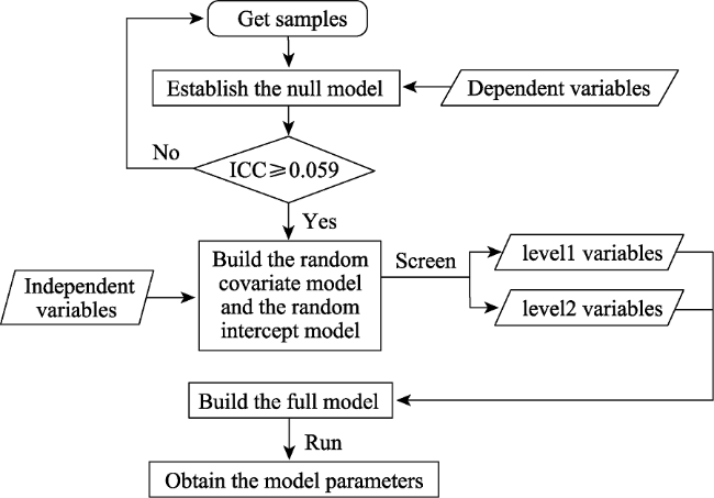
Figure 1 Flowchart of parameter acquisition based on the HGLM |
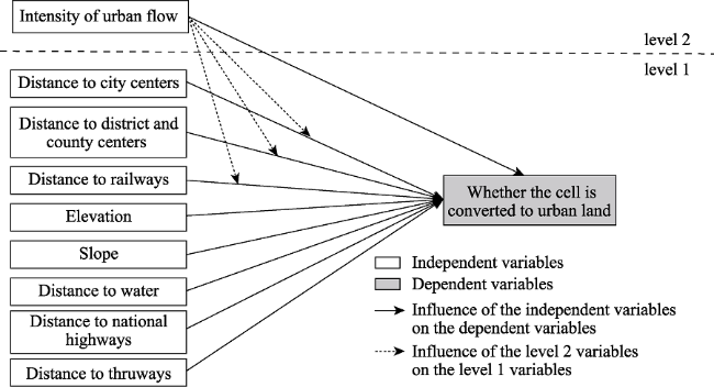
Figure 2 Framework of the HGLM-CA model |
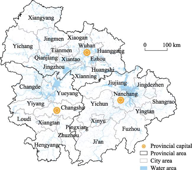
Figure 3 Location of the study area (the urban agglomeration in the middle reaches of the Yangtze River) |
Table 1 The sources of data |
| Data name | Data specification | Data source |
|---|---|---|
| Land-use data | The impervious surface data of urban areas are obtained by using the reliable impervious surface mapping algorithms and GEE platform with a resolution of 30 m×30 m. The impervious surface is regarded as urban land, while the others are non-urban land, which is resampled to 90 m ×90 m | Published by Gong et al. (2019), Tsinghua University (http://data.ess.tsinghua.edu.cn/) |
| Road data | Shapefile data including railways, thruways and national highways | Resource and Environment Science and Data Center(http://www.resdc.cn/) |
| DEM | Based on the latest SRTM V4.1 data after collation and stitching, the resolution is 90 m×90 m | Resource and Environment Science and Data Center(http://www.resdc.cn/) |
| Urban flow data | According to statistical yearbook data and big data of spatio-temporal geography, models of economic flow, population flow, traffic flow, and information flow (Wang et al., 2018; Zhai, 2019) are constructed separately to obtain the intensity of each element flow, and the weighted average of the four element flows to obtain the urban flow intensity. | See references (Zhai, 2019) |
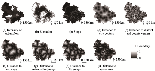
Figure 4 Driving factors of urban agglomeration spatial expansion in the middle reaches of the Yangtze River |
Table 2 ANOVA results of the HGLM |
| Fixed effect | Coefficient | Standard error | T-ratio | P-value | Random effect | Standard Deviation | Variance Component | Chi-square | P-value |
|---|---|---|---|---|---|---|---|---|---|
| γ00 | ‒2.081 | 0.120 | ‒17.337 | 0.000 | μ0 | 0.657 | 0.431 | 1571.213 | 0.000 |
Figure 5 Schematic diagram of the HGLM |
Table 3 Variable parameter identification results of the HGLM |
| Coefficient | P | Coefficient | P | ||
|---|---|---|---|---|---|
| Intercept: | Control variables: | ||||
| Level 1 intercept β0 | Elevation | ||||
| Intercept γ00 | ‒1.429 | 0.000 | Intercept γ40 | ‒0.592 | 0.000 |
| Urban flow γ01 | 0.947 | 0.000 | Slope | ||
| Independent variables: | Intercept γ50 | ‒1.764 | 0.000 | ||
| Distance to city centers β1 | Distance to water | ||||
| Intercept γ10 | ‒3.261 | 0.000 | Intercept γ60 | 0.313 | 0.315 |
| Urban flow γ11 | ‒8.176 | 0.000 | Distance to national highways | ||
| Distance to district and county centers β2 | Intercept γ70 | ‒0.486 | 0.111 | ||
| Intercept γ20 | ‒1.899 | 0.001 | Distance to thruways | ||
| Urban flow γ21 | ‒1.790 | 0.206 | Intercept γ80 | ‒0.297 | 0.391 |
| Distance to railways β3 | |||||
| Intercept γ30 | ‒1.338 | 0.048 | |||
| Urban flow γ31 | 4.752 | 0.021 | |||
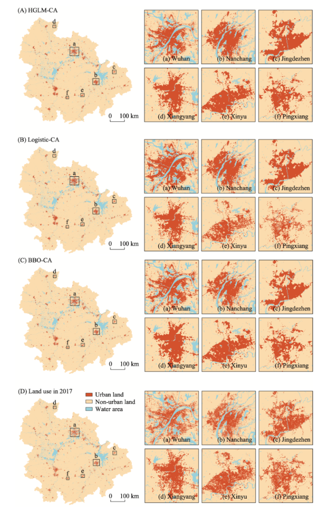
Figure 6 Comparison of the simulation results of the urban spatial expansion models in the middle reaches of the Yangtze River for 2017 |
Table 4 Comparison of the simulation accuracies of the urban spatial expansion models in the middle reaches of the Yangtze River for 2017 |
| HGLM-CA | Logistic-CA | BBO-CA | ||||||||
|---|---|---|---|---|---|---|---|---|---|---|
| OA | Kappa | FoM | OA | Kappa | FoM | OA | Kappa | FoM | ||
| Overall accuracy | Urban agglomeration | 0.99436 | 0.79872 | 0.18085 | 0.99427 | 0.79574 | 0.17374 | 0.99455 | 0.80567 | 0.19779 |
| Local accuracy | Wuhan | 0.95525 | 0.78844 | 0.14126 | 0.93924 | 0.74020 | 0.18817 | 0.94952 | 0.77246 | 0.18303 |
| Huangshi | 0.97859 | 0.81788 | 0.17746 | 0.98138 | 0.83651 | 0.16789 | 0.98146 | 0.83816 | 0.18391 | |
| Yichang | 0.99445 | 0.78486 | 0.20519 | 0.99461 | 0.78646 | 0.18571 | 0.99448 | 0.78702 | 0.21576 | |
| Xiangyang | 0.99498 | 0.82902 | 0.15516 | 0.99514 | 0.82517 | 0.03963 | 0.99475 | 0.82610 | 0.19173 | |
| Ezhou | 0.94591 | 0.69046 | 0.14923 | 0.95070 | 0.70959 | 0.15293 | 0.96023 | 0.75093 | 0.16121 | |
| Jingmen | 0.99516 | 0.82205 | 0.11262 | 0.99563 | 0.83010 | 0.01952 | 0.99485 | 0.81586 | 0.14256 | |
| Xiaogan | 0.98711 | 0.77240 | 0.17225 | 0.98773 | 0.77889 | 0.16251 | 0.98763 | 0.77942 | 0.17561 | |
| Jingzhou | 0.99185 | 0.78990 | 0.15924 | 0.99196 | 0.79076 | 0.14808 | 0.99238 | 0.80328 | 0.18866 | |
| Huanggang | 0.99170 | 0.76696 | 0.15049 | 0.99208 | 0.77326 | 0.14080 | 0.99192 | 0.77603 | 0.18343 | |
| Xianning | 0.99392 | 0.82252 | 0.12214 | 0.99464 | 0.83704 | 0.08533 | 0.99347 | 0.81337 | 0.13292 | |
| Xiantao | 0.99208 | 0.83366 | 0.00041 | 0.99204 | 0.83445 | 0.02894 | 0.99065 | 0.82169 | 0.16428 | |
| Qianjiang | 0.98856 | 0.81205 | 0.04288 | 0.98857 | 0.81206 | 0.04001 | 0.98702 | 0.80615 | 0.18890 | |
| Tianmen | 0.99343 | 0.79276 | 0.01163 | 0.99346 | 0.79249 | 0.00210 | 0.99301 | 0.80157 | 0.19527 | |
| Changsha | 0.97542 | 0.79792 | 0.19991 | 0.97230 | 0.78174 | 0.21561 | 0.97574 | 0.80148 | 0.21485 | |
| Zhuzhou | 0.98999 | 0.77736 | 0.18150 | 0.99006 | 0.77920 | 0.18720 | 0.99081 | 0.79106 | 0.18815 | |
| Xiangtan | 0.97724 | 0.75437 | 0.21572 | 0.97718 | 0.75427 | 0.21746 | 0.98161 | 0.78615 | 0.20658 | |
| Hengyang | 0.99068 | 0.77667 | 0.20602 | 0.99089 | 0.78041 | 0.20796 | 0.99141 | 0.78814 | 0.20171 | |
| Yueyang | 0.99359 | 0.81224 | 0.14242 | 0.99422 | 0.82528 | 0.12560 | 0.99355 | 0.81314 | 0.16095 | |
| Changde | 0.99417 | 0.78845 | 0.17407 | 0.99461 | 0.79653 | 0.14288 | 0.99435 | 0.79537 | 0.19085 | |
| Yiyang | 0.99511 | 0.78612 | 0.18180 | 0.99544 | 0.79554 | 0.17560 | 0.99578 | 0.80790 | 0.18663 | |
| Loudi | 0.99284 | 0.80869 | 0.19307 | 0.99392 | 0.82569 | 0.13254 | 0.99350 | 0.82162 | 0.19003 | |
| Nanchang | 0.96873 | 0.79236 | 0.25293 | 0.96683 | 0.78406 | 0.25614 | 0.97187 | 0.80732 | 0.25144 | |
| Jingdezhen | 0.98913 | 0.79545 | 0.27337 | 0.98991 | 0.80425 | 0.26468 | 0.99082 | 0.81581 | 0.25770 | |
| Pingxiang | 0.98945 | 0.79041 | 0.17084 | 0.99075 | 0.79585 | 0.01749 | 0.98967 | 0.79303 | 0.16650 | |
| Jiujiang | 0.99296 | 0.80933 | 0.21376 | 0.99308 | 0.81093 | 0.20696 | 0.99303 | 0.81233 | 0.22926 | |
| Xinyu | 0.98812 | 0.85138 | 0.27223 | 0.99066 | 0.86902 | 0.09938 | 0.98876 | 0.85730 | 0.26929 | |
| Yingtan | 0.98118 | 0.73188 | 0.23667 | 0.98301 | 0.74787 | 0.23628 | 0.98613 | 0.77889 | 0.23856 | |
| Ji’an | 0.99532 | 0.77351 | 0.20956 | 0.99562 | 0.78092 | 0.19306 | 0.99591 | 0.79410 | 0.21761 | |
| Yichun | 0.99310 | 0.81064 | 0.12226 | 0.99302 | 0.80679 | 0.09893 | 0.99240 | 0.80345 | 0.18943 | |
| Fuzhou | 0.99558 | 0.80872 | 0.17760 | 0.99598 | 0.81430 | 0.09066 | 0.99566 | 0.81252 | 0.19129 | |
| Shangrao | 0.99397 | 0.79382 | 0.16224 | 0.99446 | 0.80489 | 0.14914 | 0.99459 | 0.81160 | 0.18193 | |
| [1] |
|
| [2] |
|
| [3] |
|
| [4] |
|
| [5] |
|
| [6] |
|
| [7] |
|
| [8] |
|
| [9] |
|
| [10] |
|
| [11] |
|
| [12] |
|
| [13] |
|
| [14] |
|
| [15] |
|
| [16] |
|
| [17] |
|
| [18] |
|
| [19] |
|
| [20] |
|
| [21] |
|
| [22] |
|
| [23] |
|
| [24] |
|
| [25] |
Wuhan Statistical Bureau (WSB), 2020. 2019 Statistical bulletin of the national economic and social development of Wuhan Province. www.wuhan.gov.cn/zwgk/tzgg, 2020-03-29(006). (in Chinese)
|
| [26] |
|
| [27] |
|
| [28] |
|
| [29] |
|
| [30] |
|
| [31] |
|
| [32] |
|
| [33] |
|
/
| 〈 |
|
〉 |
