Research Articles

Dynamic evolution trend of comprehensive transportation green efficiency in China: From a spatio-temporal interaction perspective

  • MA Qifei , 1, 2 ,
  • JIA Peng , 1, 2, * ,
  • SUN Caizhi 3 ,
  • KUANG Haibo 1
Expand
  • 1. Collaborative Innovation Center for Transport Studies, Dalian Maritime University, Dalian 116026, Liaoning, China
  • 2. School of Maritime Economics and Management of Dalian Maritime University, Dalian 116026, Liaoning, China
  • 3. Institute of Marine Sustainable Development, Liaoning Normal University, Dalian 116029, Liaoning, China
* Jia Peng (1979-), Professor, specialized in multimodal transport, transportation planning and management research. E-mail:

Ma Qifei (1992-), PhD Candidate, specialized in transportation planning and management research. E-mail:

Received date: 2021-09-29

  Accepted date: 2021-11-18

  Online published: 2022-05-25

Supported by

National Key Research and Development Program of China(2019YFB1600400)

National Natural Science Foundation of China(72174035)

National Natural Science Foundation of China(71774018)

Liaoning Revitalization Talents Program(XLYC2008030)

Liaoning Provincial Natural Science Foundation Shipping Joint Foundation Program(2020-HYLH-20)

Abstract

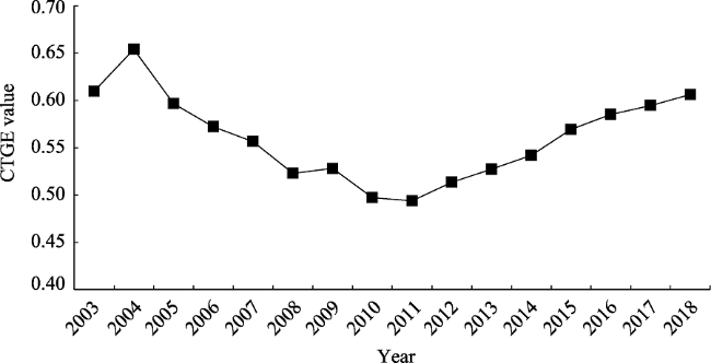
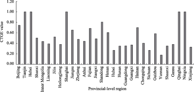
It is urgent and important to explore the dynamic evolution in comprehensive transportation green efficiency (CTGE) in the context of green development. We constructed a social development index that reflects the social benefits of transportation services, and incorporated it into the comprehensive transportation efficiency evaluation framework as an expected output. Based on the panel data of 30 regions in China from 2003-2018, the CTGE in China was measured using the slacks-based measure-data envelopment analysis (SBM-DEA) model. Further, the dynamic evolution trends of CTGE were determined using the spatial Markov model and exploratory spatio-temporal data analysis (ESTDA) technique from a spatio-temporal perspective. The results showed that the CTGE shows a U-shaped change trend but with an overall low level and significant regional differences. The state transition of CTGE has a strong spatial dependence, and there exists the phenomenon of “club convergence”. Neighbourhood background has a significant impact on the CTGE transition types, and the spatial spillover effect is pronounced. The CTGE has an obvious positive correlation and spatial agglomeration characteristics. The geometric characteristics of the LISA time path show that the evolution process of local spatial structure and local spatial dependence of China’s CTGE is stable, but the integration of spatial evolution is weak. The spatio-temporal transition results of LISA indicate that the CTGE has obvious transfer inertness and has certain path-dependence and spatial locking characteristics, which will become the major difficulty in improving the CTGE.

Cite this article

MA Qifei , JIA Peng , SUN Caizhi , KUANG Haibo . Dynamic evolution trend of comprehensive transportation green efficiency in China: From a spatio-temporal interaction perspective[J]. Journal of Geographical Sciences, 2022 , 32(3) : 477 -498 . DOI: 10.1007/s11442-022-1957-x

1 Introduction

Over decades, China’s transportation industry has accomplished great achievements. Infrastructure construction such as roads, railways, waterways, aviation and pipelines has developed rapidly, especially highways and high-speed railways, ranking first in the world. With the continuous improvement of the layout and structure of the comprehensive transportation network, the transportation support capability, service level, safety support level and equipment manufacturing capability have made remarkable progress (Jiang et al., 2020).
However, the “bottleneck” of transportation is not been completely solved, and the following problems still exist in building a comprehensive transportation system in China. Such as unbalanced transportation supply and demand, unreasonable transportation structure, low transportation efficiency, heavy traffic congestion and severe pollution (Song, 2015). Since the 21st century, human beings have faced a series of problems such as climate warming, environmental pollution and a serious waste of resources (Li et al., 2019; Zandalinas et al., 2021). The traditional economic development mode has gradually entered the bottleneck. Governments and scholars all over the world began to study and explore new development mode continuously. Green development has gradually become a hot research topic (Belmonte-Urea et al., 2021; Zindani et al., 2021). The green transportation is the inherent requirement for the healthy development of transportation, the inevitable requirement of social and economic development towards the circular economy, low-carbon economy, ecological economy and knowledge economy, and an effective measure to realize the coordinated development of transportation with economy, society and environment (Mangesh et al., 2020).
Transportation is the essential industry of the national economy, which plays an important supporting and guiding role in the development of the national economy and society. Comprehensive transportation efficiency is a crucial index to evaluate the construction quality of comprehensive transportation system, which can measure the level and potential of transportation development in a country or a region (Jia et al., 2020). Meanwhile, the concept of green development has penetrated into all fields of social economy, and the evaluation of transportation efficiency has also changed from production efficiency and operation efficiency to environment efficiency and green efficiency (Ma et al., 2021). In addition, with the wide recognition of the importance of spatial effect in social and economic development, exploring the spatial pattern characteristics of transportation efficiency have become a new hot spot in the field of transportation (Wang et al., 2020).
However, according to past literature, scholars mainly pay attention to the transportation efficiency of single transport mode and urban public transport, but lack the study of comprehensive transportation efficiency (Fitzová et al., 2018; Tamaki et al., 2019; Palander et al., 2020). In addition, most scholars only consider the economic and environmental benefits of transport services when measuring transport efficiency, while ignoring the social benefits (Liu et al., 2018; Tang et al., 2019; Xia et al., 2021).
In September 2019, the Central Committee of the Communist Party of China and the State Council issued the Outline of Building China’s Strength Transportation, which clearly put forward the construction of a safe, convenient, economical, green, and modern high-quality comprehensive transportation system, emphasizing that based on meeting the transportation supply capacity required by social and economic development, this system should pay more attention to common prosperity and the development of social and ecological civilization in the transportation field (Jiang et al., 2020; Xu et al., 2021).
Therefore, it is urgent and necessary to build a comprehensive transportation efficiency evaluation system including economic benefits, environmental regulations and social welfare. Although, Ma et al. (2021) constructed an evaluation system of comprehensive transportation green efficiency (including economic, environmental and social factors), which proved that social development index can effectively improve comprehensive transportation efficiency. Unfortunately, they did not further explore the dynamic evolution trend of comprehensive transportation green efficiency.
Meanwhile, economists believe that regional economy has obvious spatio-temporal effect in the process of development, which can promote the common growth of regional economy (Quah, 1996). Transportation is a complex system that includes many factors such as society, economy, resources and environment. Because of the differences in economic development level, resource endowment and policy orientation in different regions, the transportation efficiency is unbalanced in space. Meanwhile, due to the mobility of economic factors, the diffusion of technology, and the migration of population and goods, the transportation efficiency among different regions have a certain spatial correlation. The interaction between regions due to the flow of trade, capital, technology, information and talents play a vital role in reducing regional differences and promoting regional coordinated and sustainable development. However, the traditional spatial pattern analysis model of comprehensive transportation efficiency cuts off the time continuity of the spatial evolution process, and can not really reveal the transfer and transformation process of the spatial structure of comprehensive transportation efficiency (Liu et al., 2018). Therefore, it is of great significance to study the spatial relationship and dynamic evolution of comprehensive transportation green efficiency by integrating the elements of time and space and using the method of time-space interaction.
In view of this, we are going to solve the following problems. Is there any regional difference in the green efficiency of comprehensive transportation? Is there spatial correlations between regions, and will they influence each other? And whether the evolution characteristics of spatial differences in the future will expand or shrink? The main contributions of this article are as follows: First, according to the concept of green development and the strategic requirement of building China’s strength in transport, an evaluation system of comprehensive transportation efficiency is constructed, including economic, social and environmental factors. It integrates economic growth, resource allocation, environmental constraints and humanistic development organically, and reinterprets the connotation of comprehensive transportation green efficiency. Second, the social development index is constructed from four aspects: living standard, urbanization level, transportation level and science and technology level, and which is included in the comprehensive transportation efficiency evaluation system as the expected output. The research results well reflect the coordinated development of economy, society and environment in transportation, and enrich the theoretical framework of transportation efficiency. Third, from the perspective of spatial and temporal interaction, this study explores the spatial relationship and dynamic change regulation of the comprehensive transportation green efficiency, truly achieves the integration of “time” and “space”, and profoundly reveals the geo-dynamics of the spatial pattern of the comprehensive transportation green efficiency.
The structure of this article is as follows: Section 2 reviews the literature review of transport efficiency research. Section 3 introduces the research method and the data description. Section 4 reports the empirical results. The main conclusions and suggestions are presented in Section 5.

2 Literature review

Transportation efficiency has rich connotation and distinctive features, and has become the focus of close attention for countries in the world. Experts have made in-depth research on single transport modes (road, railway, waterway and aviation) and comprehensive transportation efficiency from different angles, and have achieved a lot of research results.
As for research methods, the existing literature on the measurement and evaluation methods of transportation efficiency are summarized, which mainly include single-factor evaluation method and total-factor evaluation method. The so-called single factor evaluation of transportation efficiency usually refers to the ratio of input and output of transportation resources. Generally, it includes index system method (Anderson et al., 1982; Levinson, 2003) and ratio analysis (Fielding et al., 1985). However, such method focuses on evaluation from a certain angle, and lacks a comprehensive index which can effectively evaluate the whole.
Total-factor evaluation usually includes data envelopment analysis (DEA) and stochastic frontier analysis (SFA), which refers to the ratio of the total output of the whole transportation system to the actual input of all factors of production (infrastructure, transportation equipment, capital, labor, energy, etc.) in the production process. For example, Michaelides et al. (2010) applied SFA and DEA to analyze the running efficiency of trolleybus in Athens and Piraeus, Greece, and compared the two analysis methods. Liu et al. (2018) explored the spatial and temporal evolution characteristics and influencing mechanisms of China’s railway transportation efficiency using the super-efficient SBM-Malmquist index model. Yuan et al. (2020) used the three-stage SBM-DEA model to measure the road transport efficiency in 31 provinces (autonomous regions and municipalities, hereafter province or region) of China, and studied the dynamic relationship between the road transport efficiency and environmental regulation. Cao et al. (2021) applied super-efficient SBM model to make a systematic analysis of the regional transportation efficiency of 30 regions in China, and considered the environmental benefits of transportation.
Infrastructure, transportation equipment, capital, labor and energy consumption are generally selected as input factors, but the selection of output indicators are different. Some early scholars only regard the added value of transportation as the expected output (Oum and Yu, 1994), which is inconsistent with the actual production process, because in actual production, the transportation system will also produce bad output such as pollution, noise and accidents. Daraio et al. (2016) found that scholars tend to use the DEA method to study transportation efficiency, but unexpected output is seldom considered in the evaluation process, which may lead to inaccurate measurement results. Then, Tone (2001) proposed a non-radial and non-angular SBM model based on the theory of the traditional DEA model, which comprehensively considered the slack variables. Subsequently, Cooper et al. (2007) proposed the SBM-undesirable model on the basis of Tone’s research, which takes into account the unexpected output. Therefore, the unexpected output has been paid more and more attention by scholars, and the evaluation of transportation efficiency has gradually shifted from economic efficiency to environmental efficiency (Chang and Zhang, 2017; Liu et al., 2020; Zhang et al., 2020). For example, Wu et al. (2016) calculated the energy efficiency and environmental efficiency of China’s transportation industry by using parallel DEA method. Tang et al. (2019) used the parallel DEA model, considering the factors of energy consumption and carbon emission, to evaluate the transportation efficiency of China’s freight transport industry. Yang et al. (2021) established a life cycle data envelopment analysis model, and measured the management performance of CO2 and PM2.5 in 30 provinces of China. Chen et al. (2021) combined four-stage data envelopment analysis with non-radical direction distance function model (NDDF), considering the bad output and environmental factors, the energy efficiency of China’s transportation sector is calculated.
To sum up, the research method of transportation efficiency has gradually changed from single-factor to total-factor evaluation method. The total-factor evaluation method can measure the allocation efficiency of transportation resources, so it is widely used by scholars at home and abroad (Cui and Li, 2014; Park et al., 2016; Yang et al., 2021). In addition, the development direction of transportation industry has changed from production efficiency, organizational efficiency and service efficiency to green efficiency.
However, the existing research still has the following deficiencies. Firstly, the related researches mainly focus on energy, environmental or carbon emission efficiency evaluation in the transport field (Chen et al., 2019; Omrani et al., 2019; Palander et al., 2020), ignoring the social benefits of transportation services. The “people-oriented” concept of green development is the development theme of the present era, and various industries pay more attention to social welfare (Zhou et al., 2019; Sun et al., 2020; Tan et al., 2021). As one of the important service industries in economy and society, the ultimate goal of transport industry is to continuously meet people’s growing transportation requirements. Therefore, it is extremely urgent and necessary to bring social welfare indicators into the evaluation framework of comprehensive transportation efficiency, pay attention to the sharing and fair distribution of transportation resources, and realize the coordinated development of transportation industry and “economy-society-environment” system (Ma et al., 2021). Secondly, the research on the spatial pattern of transportation efficiency is limited to spatial correlation and spatial difference, and most of the researches are based on cross-sectional data, which break the time continuity of the spatial evolution process and can not truly reveal the transfer and transformation process of comprehensive transportation efficiency spatial structure.
In view of this, we build a new comprehensive transportation efficiency evaluation system including economic development, environmental regulation and social welfare. Then, we apply SBM model to evaluate the CTGE from 2003 to 2018 in China, and use the spatial Markov model and exploratory spatio-temporal data analysis (ESTDA) to study the dynamic evolution trend of CTGE from a spatio-temporal interaction perspective, aiming to provide decision-making direction and theoretical support for the realization of the goal of building China’s strength transportation.

3 Methods and data

3.1 Slacks-based measure model

Data envelopment analysis (DEA) is favored by researchers in the field of efficiency evaluation, because it does not need any weight assumption, does not need to determine the input-output function relationship in advance, does not need dimensionless data processing, and can quickly deal with the comprehensive evaluation of complex systems with multiple inputs and multiple outputs (Charnes et al., 1978). Among many DEA models, the slacks-based measure (SBM) model based on slack variables can not only bring the unexpected outputs into the analysis framework, but also effectively solve the problem of input-output slack and improve the accuracy of measurement results (Guan and Xu, 2016; Sun et al., 2018). Therefore, we choose the SBM model to measure CTGE. As the SBM model has developed quite mature and widely used, the specific calculation formulas are not repeated here. Please refer to Ma et al. (2021) and Zhou et al. (2020) for details.

3.2 Spatial Markov model

The spatial Markov chain combines the traditional Markov method with the concept of “spatial lag” (Su et al., 2018; Wang et al., 2019). Based on the spatial auto-correlation theory, the spatial weight matrix was introduced to calculate the weighted average attribute value of adjacent units (spatial lag), and judge the spatial lag state of regional units (Rey and Montouri, 1999). It makes up for the deficiency that the traditional Markov chain ignores the interaction between regions, and can quantitatively analyze the spillover effect of the regional spatial lag on CTGE. Based on the spatial lag of the CTGE types in the initial year, the traditional Markov transition matrix of CTGE is decomposed into k K*K conditional transition probability matrices (see formula (1)). For the k-th conditional matrix, the element mij|k represents the spatial transition probability with the spatial lag type i of the region of year t as the background condition, and the time t belongs to the spatial transition probability from type i to the type j at the time t+1.
${M}'=\left[ \begin{matrix} {{m}_{\left. 11 \right|1}} & {{m}_{\left. 12 \right|1}} & \ldots & {{m}_{\left. 1k \right|1}} \\ {{m}_{\left. 21 \right|1}} & {{m}_{\left. 22 \right|1}} & \ldots & {{m}_{\left. 2k \right|1}} \\ \ldots & \ldots & \ldots & \ldots \\ {{m}_{\left. k1 \right|1}} & {{m}_{\left. k2 \right|1}} & \ldots & {{m}_{\left. kk \right|1}} \\ {{m}_{\left. 11 \right|2}} & {{m}_{\left. 12 \right|2}} & \ldots & {{m}_{\left. 1k \right|2}} \\ {{m}_{\left. 21 \right|2}} & {{m}_{\left. 22 \right|2}} & \ldots & {{m}_{\left. 2k \right|2}} \\ \ldots & \ldots & \ldots & \ldots \\ {{m}_{\left. k1 \right|2}} & {{m}_{\left. k2 \right|2}} & \ldots & {{m}_{\left. kk \right|2}} \\ \ldots & \ldots & \ldots & \ldots \\ \ldots & \ldots & \ldots & \ldots \\ \ldots & \ldots & \ldots & \ldots \\ \ldots & \ldots & \ldots & \ldots \\ {{m}_{\left. 11 \right|k}} & {{m}_{\left. 12 \right|k}} & \ldots & {{m}_{\left. 1k \right|k}} \\ {{m}_{\left. 21 \right|k}} & {{m}_{\left. 22 \right|k}} & \ldots & {{m}_{\left. 2k \right|k}} \\ \ldots & \ldots & \ldots & \ldots \\ {{m}_{\left. k1 \right|k}} & {{m}_{k2k}} & \ldots & {{m}_{\left. kk \right|k}} \\ \end{matrix} \right]$
To obtain the spatial Markov transition matrix of CTGE in China, we calculate the spatial lag value of region i and neighborhood j in t years, and the formula is as follows.
$La{{g}_{j}}=\sum\limits_{i=1}^{N}{{{x}_{i}}{{\omega }_{ij}}}$
where Lagj is spatial lag value of region j. xi is the efficiency value of region i. N is the number of regions. ωij is spatial weight matrix, represents the spatial relationship between region i and region j. This paper applies neighboring rook spatial weight matrix to calculate the spatial lag value. That is to say, if the areas i and j are adjacent, ωij = 1, otherwise ωij = 0. It is worth noting that in this study, we consider that Hainan Province is adjacent to Guangdong and Guangxi.

3.3 Exploratory spatio-temporal data analysis

Exploratory spatio-temporal data analysis (ESTDA) was developed from exploratory spatial data analysis (ESDA). ESDA can obtain the spatial distribution description and visual atlas of the research objects through multi-angle spatial measurement, but it ignores the time factor. In order to realize spatio-temporal coupling, Rey (2010) fully considered the characteristics of time variation and proposed the ESTDA model, which can realize the visualization of spatio-temporal interaction. Therefore, this paper analyses the spatio-temporal dynamics of CTGE by means of global spatial autocorrelation, local spatial autocorrelation, LISA time path and spatio-temporal transition methods.
3.3.1 Local indicator of spatial association time path
The local indicator of spatial association (LISA) time path integrates the time dimension, which makes the traditional static LISA dynamic. Through the time migration of the LISA coordinates in the Moran scatter plot, the paired movement of spatial unit attribute values and their spatial lag are visualized (Rey et al., 2010), thus revealing the spatio-temporal evolution of the regional CTGE in local regions, and determining the spatio-temporal dynamics of the local spatial difference in CTGE. The moving path of LISA coordinates in the Moran scatter plot of region i can be expressed as a set of vectors [(yi,1, yLi,1), (yi,2, yLi,2), …, (yi,t, yLi,t)]. yi,t represents the normalized value of CTGE in year t of region i. yLi,t is the spatial lag of region i in year t. The geometric features of LISA’s time path are usually expressed by relative length (Li) and tortuosity (δi) (Rey et al., 2011). The calculation method is as follows:
${{L}_{i}}=\frac{n\sum\limits_{t=1}^{T-1}{d({{L}_{i,t}},{{L}_{i,t+1}})}}{\sum\limits_{i=1}^{n}{\sum\limits_{t=1}^{T-1}{d({{L}_{i,t}},{{L}_{i,t+1}})}}},\text{ }{{\delta }_{i}}=\frac{\sum\limits_{t=1}^{T-1}{d({{L}_{i,t}},{{L}_{i,t+1}})}}{d({{L}_{i,1}},{{L}_{i,T}})}$
where Li and δi denote relative length and tortuosity respectively; n is the number of space units; T is the annual time interval; Li,t are LISA coordinates of unit i at time t. d(Li,t, Li,t+1) represents the movement distance of unit i from time t to t+1. d(Li,1, Li,T) represents the distance of unit i from the first year to the last year. The larger Li is, the longer the moving length is, which indicates that the local spatial structure and local spatial dependence of CTGE is more dynamic. Similarly, the larger δi is, the more curved the LISA time path is, which indicates that CTGE has a more dynamic spatial dependence direction and a more fluctuating growth process.
3.3.2 Spatio-temporal transition
Spatio-temporal transition is based on LISA time path, which embeds the moving distance, direction, concentration degree and other attributes of each spatial unit in a specific time period into the Markov chain, and further reveals the temporal change of local neighborhood spatial relationship (Ye and Rey, 2013). Spatio-temporal transition is usually divided into four types, namely, Type 0, Type 1, Type 2 and Type 3 (see Table 1), which respectively represent the local and neighbouring CTGE as stable, only local CTGE in transition, only neighbouring CTGE in transition and both local and neighbouring CTGE in transition. Type 3 can also be subdivided into two types, Type 3A and Type 3B, which respectively represent the situation of co-migration and reverse migration of local and neighbouring CTGE.
Table 1 Basic types of spatio-temporal transition
Type Spatio-temporal transition form Symbol
Type 0 Local and neighbouring CTGE as stable. HHt→HHt+1, LLt→LLt+1, HLt→HLt+1, LHt→LHt+1
Type 1 Only local CTGE in transition HHt→LHt+1, LHt→HHt+1, HLt→LLt+1, LLt→HLt+1
Type 2 Only neighbouring CTGE in transition HHt→HLt+1, LHt→LLt+1, HLt→HHt+1, LLt→LHt+1
Type 3 Both local and neighbouring CTGE in transition HHt→LLt+1, LHt→HLt+1, HLt→LHt+1, LLt→HHt+1
Rey (2010) defines space-time flux (SF) and space-time cohesion (SC) as the ratio of the number of transitions of a certain type to the number of all transitions (n) in the study period. The formula is as follows:
$SF=\frac{\text{Type }1+\text{Type }2}{n}$
$SC=\frac{\text{Type }0+\text{Type }3\text{A}}{n}$
where Type 0, Type 1, Type 2 and Type 3A represent the transition number of Type 0, Type 1, Type 2 and Type 3A, respectively. n denotes the total number of transition, n=(2018-2003)×30=450.

3.4 Index selection and data processing

On the basis of previous studies, we constructed an index system that can reflect the social development, and regarded it as an expected output in the evaluation framework of transportation efficiency, thus reflecting the coordinated development of transportation and economic-social-environmental system. Table 2 shows the evaluation index system of CTGE. The input indicators include infrastructure, capital stock, labor force and energy consumption, while output indicators include expected output (traffic added value and social development index1) (1 The social development index consists of four first-level indicators (living standard, urbanization level, transportation level and scientific technological & educational level) and 15 second-level indicators. Among them, the living standard includes GDP per capita, urban Engel’s coefficient, and rural Engel’s coefficient. Urbanization level includes the proportion of non-agricultural population, disposable income of urban residents’ families and built areas. Transportation level includes four secondary indicators: passenger turnover, cargo turnover, traffic accident and property loss in traffic accidents. The level of science and education is measured by the turnover of technology market, the number of patents granted, the proportion of science and education expenditure to government budget expenditure, the number of 10,000 college students, and illiteracy rate.)and unexpected output (carbon dioxide emission from transportation sector). Among them, the added value of transportation reflects the economic connotation of CTGE, that is, obtaining the maximum economic output with the least input of resources. Carbon emission index shows the environmental connotation of CTGE, which requires that the production process of transportation system should be based on protecting and improving the natural environment and maintaining the ecological balance, and gradually reduce the damage of unexpected output to the ecological environment. The social development index shows the social connotation of CTGE, which is people-oriented, realizing the sharing and fair distribution of transportation resources, continuously meeting the transportation needs of human development, and enhancing human well-being.
Table 2 Index system of comprehensive transportation green efficiency
Indicators First-level indicators Second-level indicators Unit
Inputs Infrastructure Total mileage of road, railway, waterway, and pipeline transportation network 10,000 kilometers
Capital stock Capital stock in transportation 100 million yuan
Labor force Individuals employed in the transportation industry Individuals
Energy consumption Energy consumption in transportation 10,000 tons of
standard coal
Outputs Expected outputs Traffic added value 100 million yuan
Social development index (SDI) -
Unexpected output CO2 emissions from transportation sector 10,000 tons
The data of infrastructure, capital stock, labor force, traffic added value and social development index are from China Statistical Yearbook, and the data of energy consumption and carbon emission are from China Energy Statistical Yearbook. Due to limited data, our research objects are 30 regions in China, excluding Hong Kong, Macao, Taiwan and Tibet, and the research period is from 2003 to 2018. Please refer to Ma et al. (2021) for the detailed calculation process of relevant indicators.

4 Results and discussions

4.1 Measurement result of comprehensive transportation green efficiency

Figures 1 and 2 show the measurement results of CTGE. Overall, CTGE shows a trend of first decreasing and then increasing in China, with an average annual efficiency below 0.65, in a low overall level (Figure 1). Specifically, from 2004 to 2011, The CTGE declined rapidly, dropped to the lowest level (0.494) in 2011, and then steadily increased. Since the 21st century, with the accelerated development of China’s market economy, the demand for transportation has increased rapidly, and input elements such as infrastructure construction, capital, manpower, and energy in the transportation industry have increased rapidly. The management mode of “heavy scale but light quality” leads to the imbalance of supply-side resource allocation in the transportation industry, and the rapid growth of unexpected output leads to a rapid decline in CTGE (Ma et al., 2021). After 2011, China attached great importance to green transportation development, accelerated structural reform on the supply side of transportation, optimized resource allocation, and significantly promoted CTGE.
Figure 1 China’s comprehensive transportation green efficiency from 2003 to 2018
Figure 2 Comprehensive transportation green efficiency in 30 provincial-level regions of China
From the regional perspective (Figure 2), only five regions (Tianjin, Hebei, Shanghai, Qinghai, Ningxia) have an efficiency value of 1, which shows that their input and output are completely effective. Only 12 regions have efficiency values are higher than the average level. Most of these regions are located in eastern part of China, which shows that there are great regional differences in China’s CTGE. Qinghai and Ningxia are located in west China, and their economic level is far lower than that of Shanghai and Tianjin in east China. There are two major reasons. One is that Qinghai and Ningxia are sparsely populated, low in economic level, backward in transportation development and inadequate in transportation resources. The other is that the unexpected output caused by less transportation demand is far lower than that in the developed eastern regions. The combination of less input and unexpected output leads to higher CTGE. It should be noted that the efficiency measured by the DEA model is relatively effective rather than the actual one, which explains why the CTGE in the underdeveloped areas is effective.

4.2 The spatio-temporal evolution trend of comprehensive transportation green efficiency

4.2.1 Result analysis on Markov state transition matrix
The quartile method is used to divide the measurement results of CTGE into four states, which are I, II, III and IV from low to high. The change of CTGE from a low-value state to a high-value state is considered to be an upward movement, and from high-value state to low-value state considered to be a downward movement. If the state of CTGE does not change, it is considered to be stable. The results are shown in Table 3 and Figure 3.
Table 3 Markov transfer matrix for comprehensive transportation green efficiency in China from 2003 to 2018
t/(t+1) n I II III IV
I 28 0.893 0.107 0 0
II 257 0.016 0.922 0.062 0
III 72 0 0.236 0.639 0.125
IV 123 0 0.008 0.065 0.927
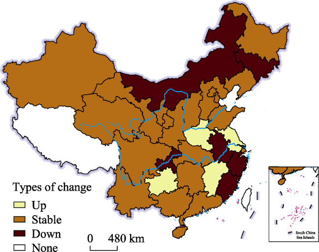
Figure 3 Spatial distribution pattern of comprehensive transportation green efficiency state transition in China
(1) Table 3 shows that the value on the diagonal is much higher than that on the non-diagonal, with the maximum value of 0.927 and the minimum value of 0.639, which indicates that the transfer of CTGE has strong stability, and the minimum probability of no transfer during the study period is 63.9%. In other words, the probability of state III changing into other states is 36.1%. In addition, the probability of CTGE at states I, II and IV remaining unchanged in the future is 89.3%, 92.2% and 92.7%, respectively, which indicates that “club integration” exists in CTGE.
(2) The transition probability between different types of CTGE is very small, and the maximum value on the non-diagonal line is 0.125, which indicates that if the CTGE of a region is Type 3A at the beginning of the study, the maximum probability of switching to other types in the following years is 12.5%. This phenomenon indicates that the probability of transition from state III to state IV is 12.5%, which shows that the CTGE in some regions has improved, and the transition from the high state to the higher state occurred. It can also be found that the transition probability between two adjacent types is greater than that of cross type, which also indicates that the transition type of CTGE is stable and gradual, but does not cross type.
(3) The CTGE is polarized between upper and lower levels. For regions with high-value at the beginning of the study, the probability of maintaining high-value in the next few years is 92.7%, and the probability of downward transition is only 7.3%. However, it is located in Type I region at the initial stage of the study, and the probability of maintaining this type is 89.3% in the next few years, and the probability of upward transition is only 10.7%, and it only transitions to Type II. This shows that the status of most low-level areas has not changed, and the regions with low-level are in urgent need of promoting, so as to promote the overall promotion of CTGE in China
(4) From the perspective of spatial distribution (Figure 3), during the study period, 20 regions (accounting for 2/3 of the total) maintained a stable state of CTGE, among which Beijing, Tianjin, Hebei, Shanghai, Qinghai and Ningxia maintained a relatively high level. Downward regions include Inner Mongolia, Jilin, Zhejiang, Anhui, Fujian, and Chongqing. Jiangsu, Jiangxi, Henan, and Guizhou are regions where the status of CTGE has moved up, which indicates that there are regional differences in the spatial and temporal evolution trend of CTGE.
4.2.2 Result analysis on spatial Markov state transition matrix
The traditional Markov chain can calculate the time evolution characteristics of China’s CTGE, but it cannot detect the effect of CTGE in the neighboring regions on this region. Therefore, this paper calculates the spatial Markov transition probability of CTGE from 2003 to 2018 in China (Table 4), takes the average level of CTGE in the surrounding regions as the spatial lag type, and draws the spatial pattern distribution map of China’s CTGE type transfer and neighborhood transfer (Figure 4).
Table 4 Spatial Markov transition matrix of comprehensive transportation green efficiency in China from 2003 to 2018
Spatial lag t n t+1
I II III IV
I I 0 0 0 0 0
II 0 0 0 0 0
III 0 0 0 0 0
IV 0 0 0 0 0
II I 28 0.893 0.107 0 0
II 130 0.031 0.915 0.084 0
III 35 0 0.228 0.686 0.086
IV 47 0 0 0.106 0.894
III I 0 0 0 0 0
II 125 0 0.936 0.064 0
III 31 0 0.258 0.581 0.161
IV 52 0 0.019 0.038 0.943
IV I 0 0 0 0 0
II 2 0 0.500 0.500 0
III 6 0 0.167 0.666 0.167
IV 24 0 0 0.042 0.958
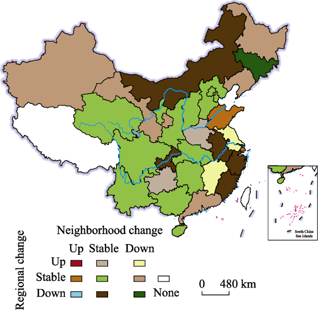
Figure 4 Spatial distribution model of state transition and neighborhood transition of comprehensive transportation green efficiency in China
Table 4 shows that there is no region with Type I as the regional background (spatial lag), so the CTGE state transition with Type I as the spatial lag condition is not considered in this paper.
(1) The condition of spatial lag has an important influence on the state transition of CTGE in China. There is synergy between regional CTGE types and neighborhood types. When the neighborhood type is I, the number of regions with Type I CTGE is obviously higher than that of other types. When the domain type is II, the number of regions with Type IV CTGE is obviously higher than other types of regions. It shows that China’s CTGE has significant spatial spillover effect, that is, CTGE depends not only on its own development level, but also on its neighboring areas.
(2) Generally speaking, the transferring downward probability of CTGE types in the region increases when it is adjacent to the region with low-value CTGE, and the transferring upward probability of CTGE types in the region increases when it is adjacent to the region with high value. That is to say, when a region is adjacent to a high-value region, the probability of the CTGE level in the region will increase. For example, Table 4 shows that the downward transition probability of Type IV is 0.042 when the neighborhood is Type IV, and increases to 0.057 and 0.106 when Type III and Type II are the neighborhood, respectively. Under the neighborhood conditions of Type IV, Type III and Type II, the upward transfer probabilities of Type III regions are 0.086, 0.161 and 0.167, respectively, which indicates that there is a significant spatial spillover effect in the development of CTGE. If the high-value regions are adjacent, the spillover effect is positive, and the probability of CTGE shifting upward increases. Similarly, if low-value regions are adjacent, the spillover effect will be negative, and the probability of CTGE downward transition will increase.
(3) For regions with Type II, under the neighborhood conditions of Type II, Type III and Type IV, the transition probabilities to Type III are 0.084, 0.064 and 0.500, respectively, while the transition probabilities to Type I are 0.031, 0 and 0, respectively. This phenomenon suggests that Type II regions tend to transition to Type III. Especially under the condition of Type IV neighborhood, this trend is more prominent. For regions with Type III, the probabilities of transition to Type IV are 0.086, 0.161 and 0.167, respectively under the conditions of Type II, Type III and Type IV of neighborhoods, and the transition probabilities to Type II are 0.228, 0.258 and 0.167 respectively. This indicates that neighboring regions have higher CTGE levels, the higher the transition probability to high-value regions, and conversely, the higher the transition probability to lower types.
The spatial spillover effect of CTGE is the result of many factors such as market, technology and policy (Wang et al., 2020). Marketization deepens the free flow of people and goods between regions, and the open economy enables regions to learn advanced technologies from other regions, especially neighbouring regions. The marginal utility of policy innovation has prompted inter-governmental institutional learning and imitation, especially the development of informatization and the continuous improvement of regional transportation infrastructure, which has reduced the flow cost of elements between regions, thus making the spatial spillover effect of CTGE more significant.

4.3 Spatial correlation analysis of comprehensive transportation green efficiency

Spatial relation is the fundamental reason for the formation and evolution of regional spatial structure. Therefore, it is necessary to consider the relevance of geospatial effects in the study of regional CTGE spatio-temporal evolution.
4.3.1 Global spatial autocorrelation analysis
This paper calculates and investigates the global Moran’s I and the global spatial correlation of CTGE from 2003 to 2018 by using the GeoDa software. Table 5 shows that the global Moran’s I of CTGE in China is positive from 2003 to 2018, and it is significant in other years except 2009, which indicates that CTGE has a strong agglomeration effect (positive correlation) in space. That is to say, the high (low) value regions of the CTGE tend to be adjacent in space.
Table 5 Global Moran’s I of comprehensive transportation green efficiency in China
Year Moran’s I z p Year Moran’s I z p
2003 0.2335 2.3390 0.008 2011 0.1703 2.3493 0.040
2004 0.2187 2.1630 0.017 2012 0.1804 1.9644 0.028
2005 0.2120 2.1120 0.015 2013 0.1317 1.5070 0.074
2006 0.1258 1.3507 0.088 2014 0.1547 1.6905 0.049
2007 0.1227 1.3727 0.083 2015 0.1311 1.4382 0.073
2008 0.1123 1.2777 0.097 2016 0.1458 1.5770 0.054
2009 0.0974 1.1687 0.111 2017 0.2403 2.3170 0.013
2010 0.1527 1.6420 0.062 2018 0.2456 2.4775 0.007
4.3.2 Local spatial autocorrelation analysis
Since the global autocorrelation Moran’s I can not reflect the spatial agglomeration characteristics of a specific region, this paper draws the LISA agglomeration map of the CTGE in 2003, 2008, 2013 and 2018 by combining Moran scatter plot and local Moran’s I to explore whether there is a local agglomeration phenomenon of CTGE in China (Figure 5).
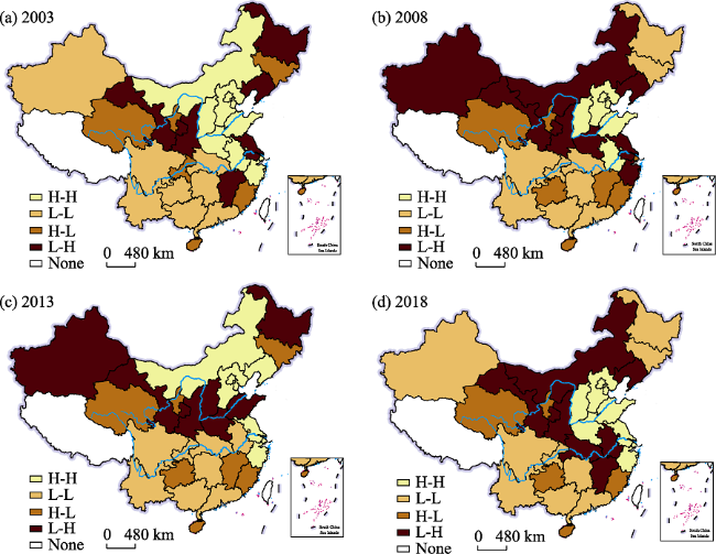
Figure 5 The LISA aggregation map of comprehensive transportation green efficiency in China
Through the comparative analysis of the four agglomeration types, we found that the high-value agglomeration centers (H-H agglomeration) of CTGE are relatively stable in north China and the Yangtze River Delta, while the low-value agglomeration centers (L-L agglomeration) gradually spread from the south of the Yangtze River to the northeast. During the research period, the number of L-H agglomeration increased slightly, while the spatial distribution pattern changed greatly. In 2003, the regions of L-H agglomeration were scattered in eastern, northeastern and northwestern China. In 2008, we found that the low-value isolated centers of L-H agglomeration were mainly in north China and the Yangtze River Delta. In 2013, low-value isolation centers were concentrated in Xinjiang, Heilongjiang and Yellow River Basin. In 2018, two isolated centers with low value were formed in the middle reaches of the Yellow River and the Yangtze River. The number of high-value isolated centers (H-L clusters) decreased slightly during the study period, but their spatial distribution pattern did not change much, and spread in eastern, central and western China in a divergent state. Generally speaking, the H-H concentration and L-L concentration are concentrated and distributed in a large number, while the L-H concentration and H-L concentration are divergent and distributed in a small number.

4.4 The spatio-temporal dynamic pattern of comprehensive transportation green efficiency

4.4.1 Local indicator of spatial association time path geometry features
The relative length and tortuosity of LISA time path can better reveal the dynamic and spatial correlation fluctuation of the local spatial structure of CTGE. In this paper, the length and tortuosity of LISA time path for CTGE from 2003 to 2018 are divided into four grades: low-relative length (low-tortuosity), medium-relative length (medium-tortuosity), higher-relative length (higher-tortuosity), and high-relative length (high-tortuosity). The relative length and tortuosity of LISA time path are visualized by ArcGIS 10.2 software, and the results are shown in Figure 6.
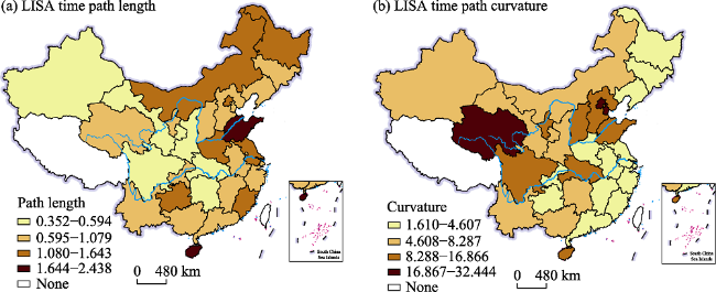
Figure 6 Spatial distribution of geometry features of LISA time path in China
According to the relative length of LISA time path (Figure 6a), there are 20 regions below the average level (Li<1), accounting for 66.67% of the regional proportion, which shows that the local spatial structure of CTGE has strong stability. In terms of spatial distribution, the long-path (1.080-2.438) regions are scattered, including Beijing, Heilongjiang, Inner Mongolia, Shandong and Henan in the north and Guizhou, Hainan and Fujian in the south. The short-path (0.352-1.079) regions are relatively concentrated in spatial distribution, mainly in north, northwest and southeast China. The reason is that the transportation level in these places is generally low, and the transportation service is mainly road transportation with high consumption and high emission, which leads to low CTGE and hard to change. Specifically, the relative length between Shandong and Hainan is 1.644-2.438, which is a high-relative length region, and its local space structure is extremely unstable. The seven provinces of Beijing, Heilongjiang, Inner Mongolia, Jiangsu, Fujian, Henan and Guizhou are higher-relative length, ranging from 1.080 to 1.643, and its local spatial pattern is dynamic. The relative length of Hebei, Tianjin, Shanxi, Liaoning, Jilin, Guangdong, Shanghai and Zhejiang is between 0.595 and 1.079, which is a medium-relative length region, indicating that the local spatial structure is relatively stable. These regions are mainly concentrated in northeast, north China and south of the Yangtze River. Xinjiang, Gansu, Sichuan, Shaanxi, Hunan and Hubei are low-relative length, with path length ranging from 0.353 to 0.874, which is mainly concentrated in western China and the middle reaches of the Yangtze River.
According to the tortuosity of LISA time paths (Figure 6b), 19 regions are smaller than the average tortuosity (8.262), accounting for 63.33% of the regional proportion, indicating that the local spatial dependence of CTGE is relatively stable. From the spatial distribution of tortuosity, the tortuosity of LISA time path of CTGE is in a central distribution structure, and it is decreasing from Beijing to Tianjin. Specifically, the regions with low-tortuosity (1.610-4.607) are mainly distributed in the northeast and southeast of China, and have the greatest stability in the direction of spatial dependence, which is related to the low level of CTGE in this region. The similar development level leads to weak fluctuation of local spatial dependence change process. The regions with high-tortuosity (16.867-32.444) are Beijing, Tianjin and Qinghai, which reflects that these regions have the most significant fluctuation and very dynamic spatial change process in the direction of spatial dependence on their neighbouring regions. The regions with medium-tortuosity (4.608-8.287) are mainly concentrated in the northwest and southwest regions of China. The provinces with higher- tortuosity (8.288-16.866) are mainly concentrated in north China and the middle reaches of the Yangtze River, which include Hebei, Shanxi, Shandong, Sichuan and Hubei provinces, indicating that CTGE has a strong local spatial dependence.
4.4.2 Local indicator of spatial association time path movement direction
The direction of the LISA time path can represent the comprehensive characteristics of the evolution of local spatial pattern of an element. This paper compares the specific positions of LISA scatter plot of CTGE in 2003 and 2018, calculates the moving direction of the LISA coordinates in various regions, and divides them into four types: win-win type (0°-90°), loss-win type (90°-180°), loss-loss type (180°-270°) and win-loss type (270°-360°). Among them, the win-win type indicates that CTGE of the province and its neighbors shows a positive cooperative growth. The lost-win type indicates that the province itself shows a low growth trend, while the neighborhood offers a high growth trend, and vice versa.
In terms of LISA time path transition direction (Figure 7), there are 13 regions with coordinated transition of CTGE, accounting for 43.33% of the total number of regions, which indicates that the integration of spatial pattern evolution of CTGE is weak. In the process of spatial evolution, coordinated spatial growth and spatial competition coexist. Among them, there are eight regions which are growing together, mainly distributed in the North China Plain and the Yangtze River Delta. The CTGE in these areas is generally high, showing obvious characteristics of coordinated and high-speed growth. There are five growing regions with negative cooperativity, which are concentrated in northeast China, Inner Mongolia, and Gansu, showing the characteristics of coordinated low-speed growth.
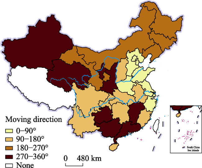
Figure 7 Spatial distribution of LISA time path moving direction in China
4.4.3 Analysis of spatio-temporal transition
The physical change characteristics of the LISA time path reveal the movement trend of the regional CTGE’s LISA coordinates, but it can not reflect the mutual transformation of local spatial association types in CTGE’s LISA coordinates. Therefore, this paper uses the spatio-temporal transition method proposed by Rey (2010) to further describe the transfer characteristics and evolution types of the local spatial association types of CTGE in China. The results are shown in Table 6.
Table 6 Spatio-temporal transition matrices of local Moran’s I
t/t+1 H-H L-H L-L H-L Type n Proportion SF SC
H-H 0.857 0.101 0 0.042 Type0 387 0.860 0.136 0.864
L-H 0.095 0.827 0.069 0.009 Type1 34 0.076 - -
L-L 0 0.060 0.907 0.033 Type2 27 0.060 - -
H-L 0.053 0.011 0.064 0.872 Type3 2 0.004 - -
Table 6 shows that the diagonal value of the probability transfer matrix is much larger than that on the non-diagonal, with the maximum value of 0.907 and the minimum value of 0.827 on the diagonal, indicating that the spatial structure between regions of CTGE is relatively stable, and the transition possibility different types are small. China’s CTGE has obvious transfer inertness. Among the different types of transitions, HHt→LHt+1, LHt→ HHt+1 and LHt→LLt+1 have the highest transition probabilities, which are 0.101, 0.095 and 0.069, respectively. The transition probabilities of the other types are low, which indicates that the spatial structure of CTGE is relatively stable. Turning to the spatio-temporal transition probability, Moran’s I scatter points with Type 0 is the highest during the research period, reaching 387 times, accounting for 86%. That is to say, the probability of Moran’s I scatter points staying in the same quadrant (Type 0) is 86%. The transition frequency of Type 3 is the least, only two times, accounting for only 0.4%, while the transition frequency of Type 1 and Type 2 is 34 times and 27 times, respectively, with probabilities of 0.076 and 0.060. According to formulas (4) and (5), the spatio-temporal conversion and spatio-temporal convergence probability of CTGE are calculated. The spatio-temporal cohesion (SC) of Moran’s I is 0.864, which indicates that the probability of no spatio-temporal transition in China’s comprehensive transportation green efficiency is 86.4%, and the space-time flux (SF) probability of Moran’s I is only 13.6%, indicating that the spatial agglomeration of CTGE has strong path dependence and locking characteristics.

5 Conclusions and implications

5.1 Conclusions

Using the SBM, spatial Markov and ESTDA model, we calculated CTGE of 30 provinces from 2003 to 2018 in China, and explored the spatio-temporal interaction characteristics of its spatial pattern. The major conclusions are as follows:
(1) The green efficiency of China’s comprehensive transportation shows a U-shaped trend (first decreasing and then increasing), but the overall level is low. The efficiency values are ranging from 0.179 to 1, which is quite different in regions. The spatial distribution roughly presented eastern > western > central regions, without economic spatial regularity.
(2) The transfer of CTGE in China showed a steady and gradual feature, but there is also a polarization phenomenon of “the better, the worse”. The spatial spillover effect of CTGE in China is obvious. Generally speaking, if it is close to a high-level region, the upward transfer probability of CTGE will increase, while if it is close to the low-level region, the upward transfer probability of CTGE will decrease.
(3) During the study period, the CTGE has significant positive spatial correlation and spatial agglomeration characteristics, and spatial convergence (degree of agglomeration) shows a trend of decreasing at first and then increasing. H-H agglomeration and L-L agglomeration are large in number and concentrated in distribution, while L-H agglomeration and H-L agglomeration are small in number and dispersed.
(4) The LISA time path geometry features show that the evolution process of local spatial structure and local spatial dependence of CTGE is stable, but the integration of spatial evolution is weak, and spatial cooperation growth and spatial competition coexist. The results of LISA spatio-temporal transition show that CTGE has obvious transfer inertness, and has certain characteristics of path dependence and spatial locking, which will become a major difficulty that hinders the improvement of CTGE.

5.2 Policy implications

According to the conclusions, the following implications and enlightenment can be drawn.
(1) Optimize transportation structure to improve CTGE. Although CTGE has been rising in recent years, its overall level is still relatively low. The reason lies in the lack of effective links among various modes of transportation, which leads to unbalanced resource allocation and serious waste at the input end of comprehensive transportation system. Therefore, optimizing the transportation structure, strengthening the effective connection of various modes of transportation are the primary problems facing the construction of high-quality comprehensive transportation systems. Concrete measures are as follows. The development of new energy automobile industry using pure electricity, hybrid power, and hydrogen energy and having reduced consumption of fossil fuels, such as gasoline and diesel, should be promoted. New modes of transport organization, such as multimodal transport, swap trailer transport, etc., should be adopted to promote container transport and reduce transport intensity. Furthermore, it would be important to optimize the transport structure, vigorously promote highway to waterway and railway transport, and improve the green efficiency of comprehensive transportation.
(2) Making differentiated policy to improve CTGE. The evolution process of local spatial structure of CTGE in China has a strong stability. For low-efficiency areas, to break this stable process, it is necessary to optimize the traffic structure, scientifically plan the comprehensive traffic layout, and strengthen the connection between various modes of transportation. At the same time, it is necessary to intensify scientific and technological research and development, so as to make comprehensive transportation develop in the direction of intelligence, promote the development of transportation from resource input to technological innovation, and ensure that the expected output is increased and carbon emissions are reduced. For high-efficiency areas, it is necessary to keep the stability of CTGE local spatial structure and the evolution process of spatial dependence, and on this basis, continuously optimize the allocation of transportation production materials and improve the utilization rate of resources. On the other hand, it is necessary to give full play to the demonstration and leading role of efficient areas, improve the diffusion and spillover effects of advanced technology and management experience, and realize the cross-regional coordinated promotion of comprehensive transportation green efficiency.
(3) Narrow regional differences to improve CTGE. On the one hand, due to natural conditions, resource endowments, economic foundation and other factors, the speed and quality of traffic development in different areas are quite different. On the other hand, the difference in the degree and effect of policy implementation leads to the widening gap of CTGE in different regions. Therefore, under the guidance of the building national strength in transportation, local governments should strive to promote the development of comprehensive transportation system, formulate a coordinated development strategy of inter-regional comprehensive transportation, and establish a sound linkage mechanism for transportation cooperation, such as the integrated development of Beijing-Tianjin-Hebei, so as to achieve coordinated development of regional transportation while improving the green efficiency of their comprehensive transportation. In addition, it is necessary to strengthen the exchange and cooperation of talents, capital and technology among regions, give full play to the leading role of the developed regions around Bohai Sea, Yangtze River Delta and Pearl River Delta in the central and western regions and northeastern China, promote the spillover of new technologies, methods and knowledge, narrow regional differences, and realize the overall improvement of comprehensive transportation green efficiency.
In any case, this study has some limitations that merit mention. Firstly, there is no uniform standard for the construction of the social dimension index system at present. The index system established in this paper is not comprehensive, the calculation results are rough, and few indicators reflecting the government management decision-making level are involved. Further development and improvement are needed. Secondly, considering the availability and convenience of the data, all the data in this paper come from the National Bureau of Statistics, and the calculation results are relatively rough, so it is necessary to further refine the comprehensiveness and accuracy of the data in the future. Thirdly, this paper takes provincial units as the research object, and the research scale is large, so it is impossible to explore regional differences. In the future, it is necessary to refine the granularity and evaluate the CTGE in China with prefecture-level cities as evaluation units.
Nevertheless, we hope that our research results can provide sufficient theoretical support for the establishment of high-quality comprehensive transportation systems to realize the rationalization of transportation resources and the coordinated development of the regional economy.
[1]
Anderson S C, Fielding G L, 1982. Comparative analysis of transit performance. Final Report for the US Department of Transportation, Washigton, DC.

[2]
Belmonte-Urea L J, Plaza-Beda J A, Vazquez-Brust D et al., 2021. Circular economy, degrowth and green growth as pathways for research on sustainable development goals: A global analysis and future agenda. Ecological Economics, 185(19), 107050: 1-17.

[3]
Cao X D, Wang J J, Chen C C, 2021. Efficiency of traffic structure based on SBM-Tobit-GWR model. Journal of Southwest Jiaotong University, 56(3): 594-601. (in Chinese)

[4]
Chang Y T, Zhang N, 2017. Environmental efficiency of transportation sectors in China and Korea. Maritime Economics & Logistics, 19(1): 68-93.

[5]
Charnes A, Cooper W, Roodes E, 1978. Measuring the efficiency of decision making units. European Journal of Operational Research, 2(6): 429-444.

DOI

[6]
Chen Y F, Cheng S Y, Zhu Z T, 2021. Measuring environmental-adjusted dynamic energy efficiency of China’s transportation sector: A four-stage NDDF-DEA approach. Energy Efficiency, 14(3): 1-14.

DOI

[7]
Cheng Y, Lv K J, Wang J et al., 2019. Energy efficiency, carbon dioxide emission efficiency, and related abatement costs in regional China: A synthesis of input-output analysis and DEA. Energy Efficiency, 12(4): 863-877.

DOI

[8]
Cooper W W, Seiford L M, Tone K, 2007. Data Envelopment Analysis. 2nd ed. Boston: Kluwer Academic Publishers.

[9]
Cui Q, Li Y, 2014. The evaluation of transportation energy efficiency: An application of three-stage virtual frontier DEA. Transportation Research Part D: Transport and Environment, 29: 1-11.

DOI

[10]
Daraio C, Diana M, Costa F D et al., 2016. Efficiency and effectiveness in the urban public transport sector: A critical review with directions for future research. European Journal of Operational Research, 248(1): 1-20.

DOI

[11]
Fielding G J, Babitsky T T, Brenner M E, 1985. Performance evaluation for bus transit. Transportation Research Part A: Policy and Practice, 19(1): 73-82.

DOI

[12]
Fitzová H, Matulová M, Tomeš Z, 2018. Determinants of urban public transport efficiency: Case study of the Czech Republic. European Transport Research Review, 10(2), 42: 1-11.

DOI

[13]
Guan W., Xu S.T., 2016. Study of spatial patterns and spatial effects of energy eco-efficiency in China. Journal of Geographical Sciences, 26(9): 1362-1367.

DOI

[14]
Jia P, Hu Y, Yuan S et al., 2020. A research on the comprehensive transportation efficiency and its spatial relevancy in China’s provinces. Science Research Management, 41(9): 219-229. (in Chinese)

[15]
Jiang X H, Ma J X, Zhu H Z et al., 2020. Evaluating the carbon emissions efficiency of the logistics industry based on a super-SBM model and the Malmquist index from a strong transportation strategy perspective in China. International Journal of Environmental Research and Public Health, 17(22), 8459: 1-19.

DOI

[16]
Levinson D, 2003. Perspectives on efficiency in transportation. International Journal of Transport Management, 1(3): 145-155.

DOI

[17]
Li Y, Du Q, Lu X R et al., 2019. Relationship between the development and CO2 emissions of transport sector in China. Transportation Research Part D: Transport and Environment, 74: 1-14.

DOI

[18]
Liu B Q, Wu W, Su Q et al., 2018. Spatio-temporal evolution characteristics and mechanism of railway efficiency in China. Geographical Research, 37(3): 512-526. (in Chinese)

[19]
Liu H W, Wu J, Chu J F, 2018. Environmental efficiency and technological progress of transportation industry-based on large scale data. Technological Forecasting and Social Change, 144: 475-482.

DOI

[20]
Liu H W, Yang R L, Wang Y Q et al., 2020. Measuring performance of road transportation industry in China in terms of integrated environmental efficiency in view of streaming data. Science of the Total Environment, 727, 138675: 1-13.

[21]
Ma Q F, Jia P, Kuang H B, 2021. Green efficiency changes of comprehensive transportation in China: Technological change or technical efficiency change? Journal of Cleaner Production, 304, 127115: 1-11.

[22]
Mangesh V L, Tamizhdurai P, Krishnan P S et al., 2020. Green energy: Hydroprocessing waste polypropylene to produce transport fuel. Journal of Cleaner Production, 276, 124200: 1-16.

[23]
Michaelides P G, Belegri-Roboli A, Marinos T, 2010. Evaluating the technical efficiency of trolley buses in Athens, Greece. Journal of Public Transportation, 13(4): 93-109.

[24]
Omrani H, Shafaat K, Alizadeh A, 2019. Integrated data envelopment analysis and cooperative game for evaluating energy efficiency of transport sector: A case of Iran. Annals of Operations Research, 274(1): 471-499.

DOI

[25]
Oum T, Yu C, 1994. Economic efficiency of railways and implications for public policy: A comparative study of the OECD countries’ railways. Journal of Transport Economics and Policy, 28(2): 121-138.

[26]
Palander T, Haavikko H, Kortelainen E et al., 2020. Comparison of energy efficiency indicators of road transportation for modeling environmental sustainability in “Green” circular industry. Sustainability, 12(7), 2740: 1-22.

DOI

[27]
Park Y S, Lim S H, Egilmez G et al., 2016. Environmental efficiency assessment of U.S. transport sector: A slack-based data envelopment analysis approach. Transportation Research Part D: Transport and Environment, 61: 152-164.

DOI

[28]
Quah D T, 1996. Regional convergence clusters across Europe. European Economic Review, 40(3): 951-958.

DOI

[29]
Rey S J, 2010. Spatial empirics for economic growth and convergence. Geographical Analysis, 33(3): 195-214.

DOI

[30]
Rey S J, Montouri B D, 1999. US regional income convergence: A spatial econometric perspective. Regional Studies, 33(2): 143-156.

[31]
Rey S J, Murray A T, Anselin L, 2011. Visualizing regional income distribution dynamics. Letters in Spatial and Resource Sciences, 4(1): 81-90.

DOI

[32]
Rey S J, Ye X, Páez A et al., 2010. Comparative Spatial Dynamics of Regional Systems. Berlin Heidelberg: Springer.

[33]
Song J N, 2015. Research on formation mechanism and evaluation of comprehensive transport efficiency [D]. Xi’an: Chang’an University. (in Chinese)

[34]
Su W S, Liu Y Y, Wang S J et al., 2018. Regional inequality, spatial spillover effects, and the factors influencing city-level energy-related carbon emissions in China, Journal of Geographical Sciences, 28(4): 495-513.

DOI

[35]
Sun C Z, Ma Q F, Zhao L S, 2020. Analysis of driving mechanism based on a GWR model of green efficiency of water resources in China. Acta Geographica Sinica, 75(5): 1022-1035. (in Chinese)

[36]
Sun J S, Wang Z H, Li G, 2018. Measuring emission-reduction and energy-conservation efficiency of Chinese cities considering management and technology heterogeneity. Journal of Cleaner Production, 175: 561-571.

DOI

[37]
Tamaki T, Nakamura H, Fujii H et al., 2019. Efficiency and emissions from urban transport: Application to world city-level public transportation. Economic Analysis and Policy, 61: 1-9.

DOI

[38]
Tan S K, Hu B X, Kuang B et al., 2021. Regional differences and dynamic evolution of urban land green use efficiency within the Yangtze River Delta, China. Land Use Policy, 106, 105449: 1-10.

[39]
Tang T B, You J X, Sun H et al., 2019. Transportation efficiency evaluation considering the environmental impact for China’s freight sector: A parallel data envelopment analysis. Sustainability, 11(18), 5108: 1-24.

DOI

[40]
Tone K, 2001. A slacks-based measure of efficiency in data envelopment analysis. European Journal of Operational Research, 130(3): 498-509.

DOI

[41]
Wang L K, Peng C, Shi W M et al., 2020. Carbon dioxide emissions from port container distribution: Spatial characteristics and driving factors. Transportation Research Part D: Transport and Environment, 82, 102318: 1-11.

[42]
Wang S J, Gao S, Huang Y Y et al., 2020. Spatio-temporal evolution and trend prediction of urban carbon emission performance in China based on super-efficiency SBM model. Acta Geographica Sinica, 75(6): 1316-1330. (in Chinese)

[43]
Wang S J, Huang Y Y, Zhou Y Q, 2019. Spatial spillover effect and driving forces of carbon emission intensity at the city level in China. Journal of Geographical Sciences, 29(2): 231-252.

DOI

[44]
Wu J, Zhu Q Y, Chu J F et al., 2016. Measuring energy and environmental efficiency of transportation systems in China based on a parallel DEA approach. Transportation Research Part D: Transport and Environment, 48: 1-13.

DOI

[45]
Xia Z C, Guo Z J, Wang W Y et al., 2021. Joint optimization of ship scheduling and speed reduction: A new strategy considering high transport efficiency and low carbon of ships in port. Ocean Engineering, 233, 109224: 1-13.

[46]
Xu Y, Fan J Q, Xu H C, 2021. Study on the operation efficiency of toll roads in China from the perspective of scale economy. Journal of Advanced Transportation, 8830521: 1-15.

[47]
Yang F, Choi Y, Lee H, 2021. Life-cycle data envelopment analysis to measure efficiency and cost-effectiveness of environmental regulation in China’s transport sector. Ecological Indicators, 126, 107717: 1-8.

[48]
Ye X, Rey S J, 2013. A framework for exploratory space-time analysis of economic data. The Annals of Regional Science, 50(1): 315-339.

DOI

[49]
Yuan C W, Sun L, Li T T et al., 2020. Research on the relationship between environmental regulation and highway transportation efficiency based on PVAR model. Environmental Science & Technology, 43(5): 221-229. (in Chinese)

[50]
Zandalinas S I, Fritschi F B, Mittler R, 2021. Global warming, climate change, and environmental pollution: Recipe for a multifactorial stress combination disaster. Trends in Plant Science, 26(6): 588-599.

DOI

[51]
Zhang J X, Cai W Y, Philbin S P et al., 2020. Measuring the capacity utilization of China’s transportation industry under environmental constraints. Transportation Research Part D: Transport and Environment, 85, 102450: 1-21.

[52]
Zhou L, Che L, Zhou C H, 2019. Spatio-temporal evolution and influencing factors of urban green development efficiency in China. Acta Geographica Sinica, 74(10): 2027-2044. (in Chinese)

[53]
Zhou L, Zhou C H, Che L et al., 2020. Spatio-temporal evolution and influencing factors of urban green development efficiency in China. Journal of Geographical Sciences, 30(5): 724-742.

DOI

[54]
Zindani D, Maity S R, Bhowmik S, 2021. Extended TODIM method based on normal wiggly hesitant fuzzy sets for deducing optimal reinforcement condition of agro-waste fibers for green product development. Journal of Cleaner Production, 301, 126947: 1-22.

Options
Outlines

/